
Numerical Simulation for the Evolution of Internal Solitary Waves Propagating over Slope Topography


Abstract
:1. Introduction
2. Numerical Simulation
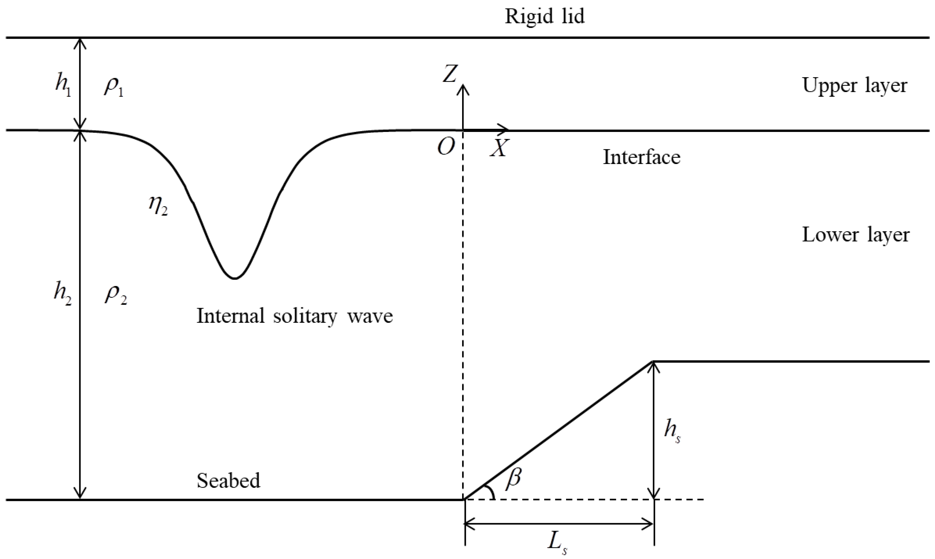
2.1. Physical Model
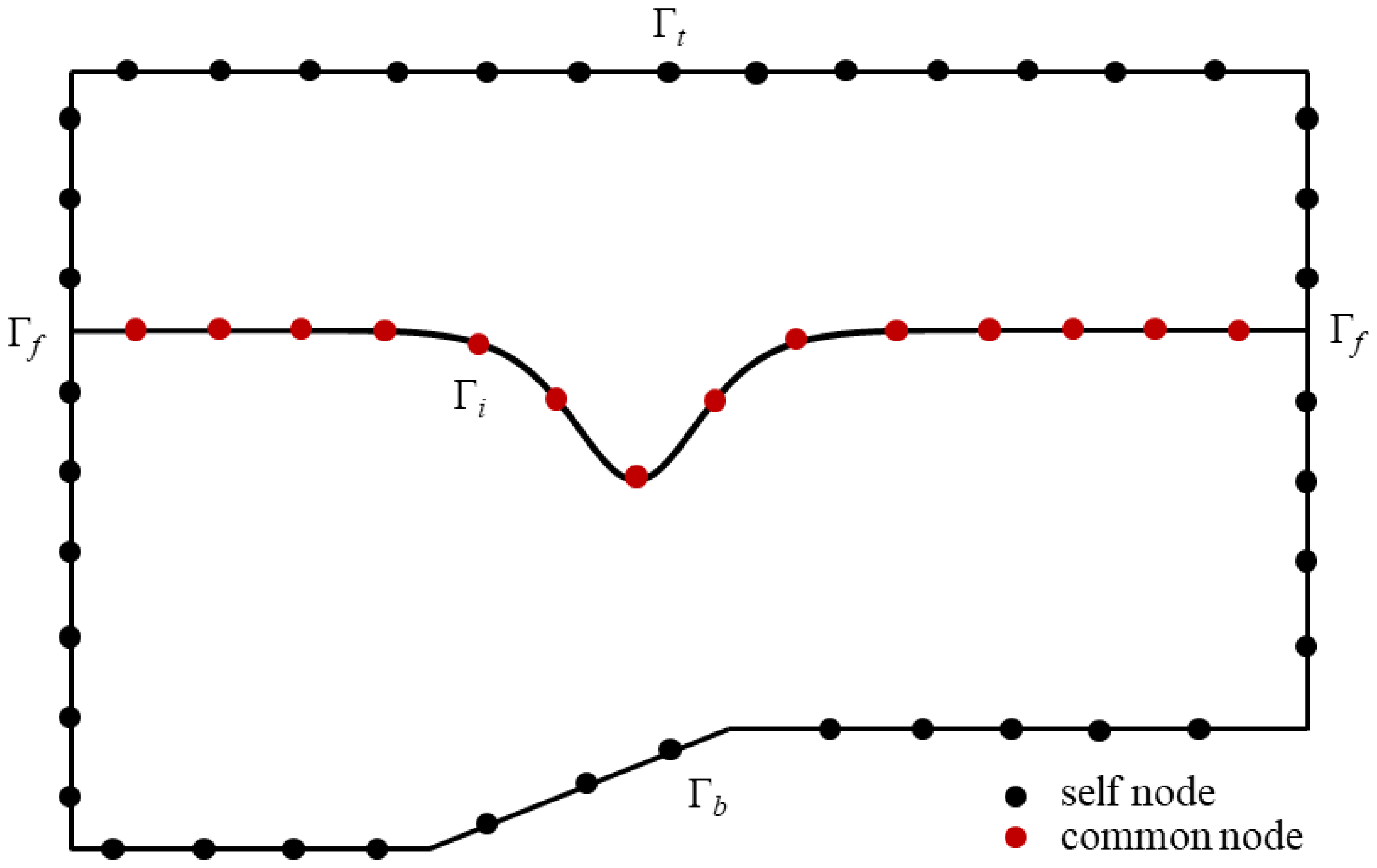
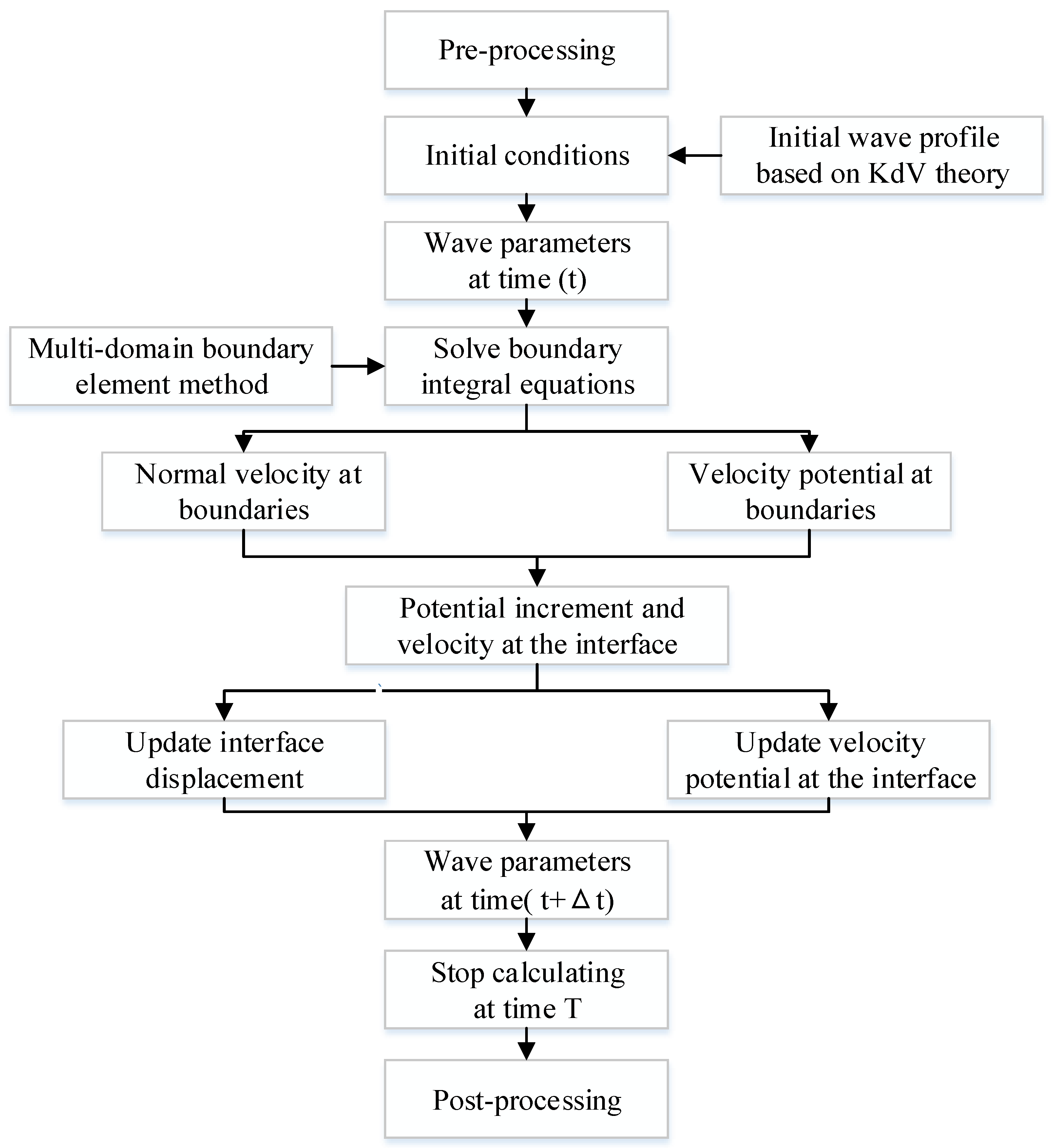
2.2. Numerical Model
3. Results
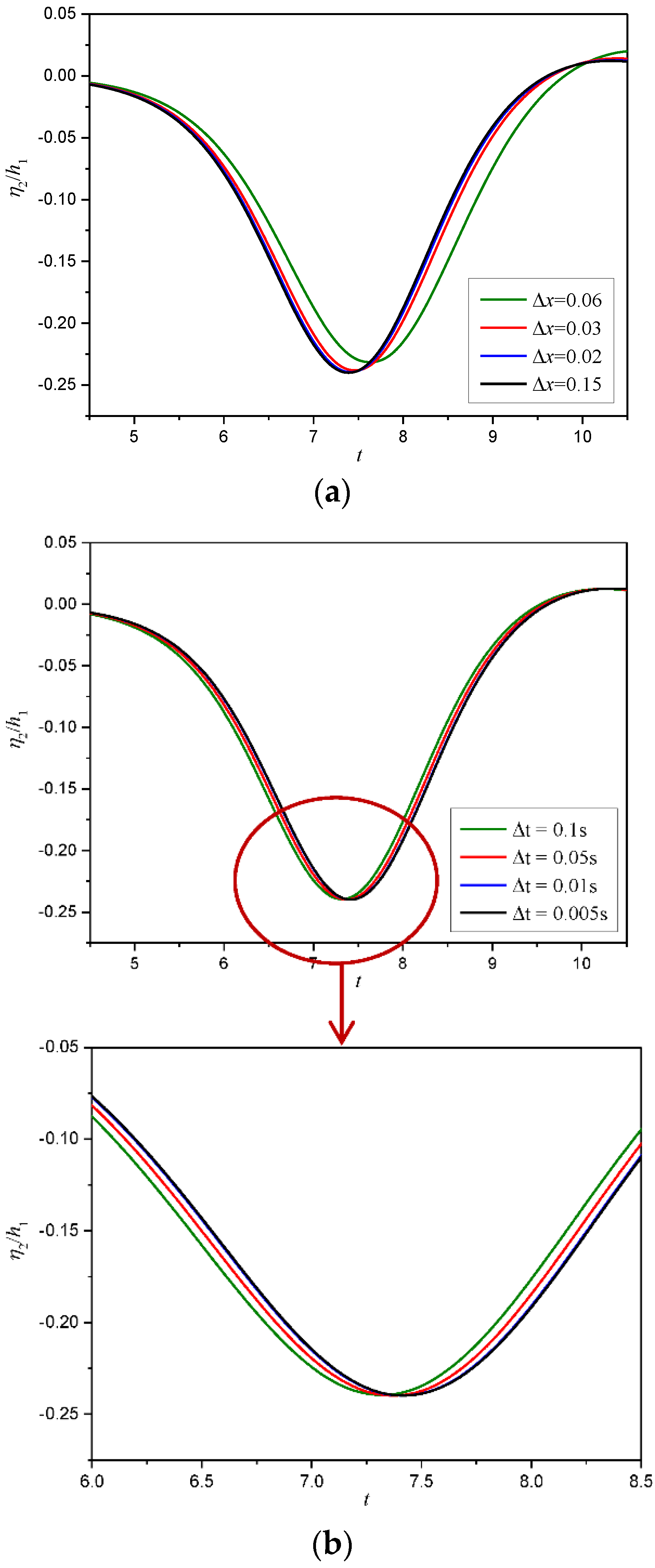
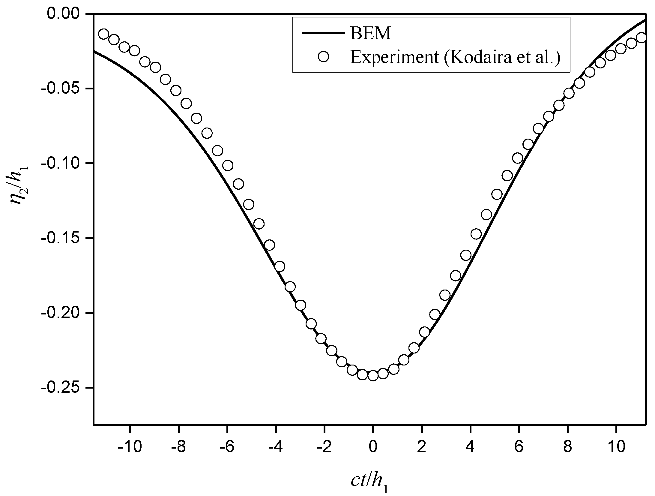
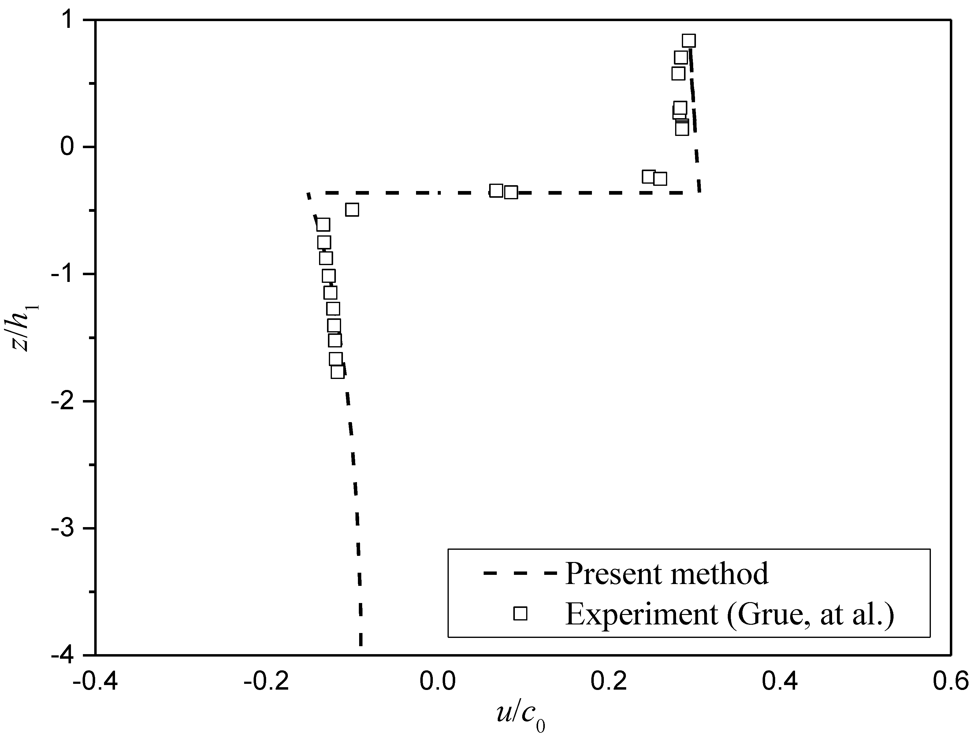
3.1. Numerical Model Validation
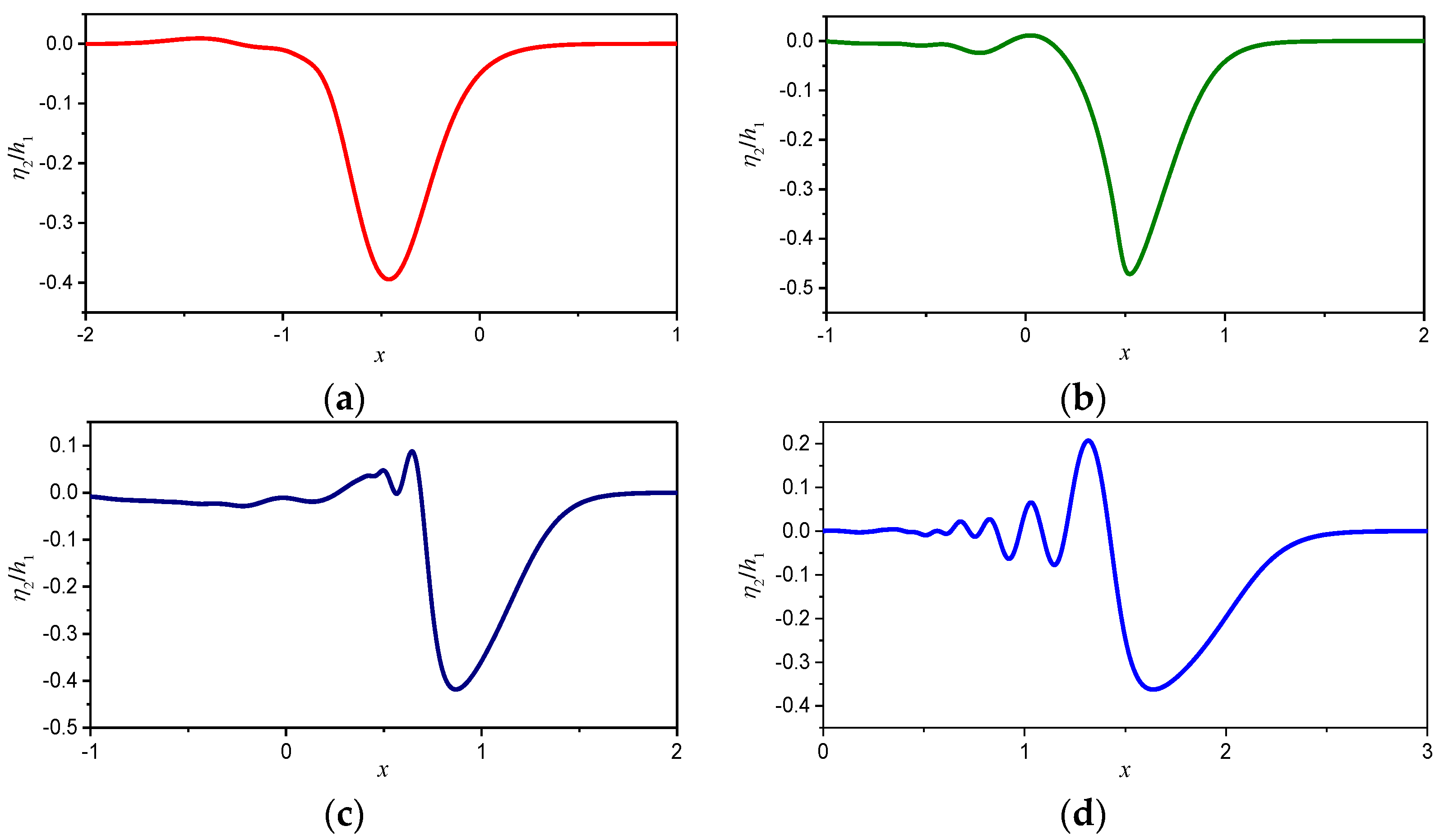
3.2. Wave Evolution
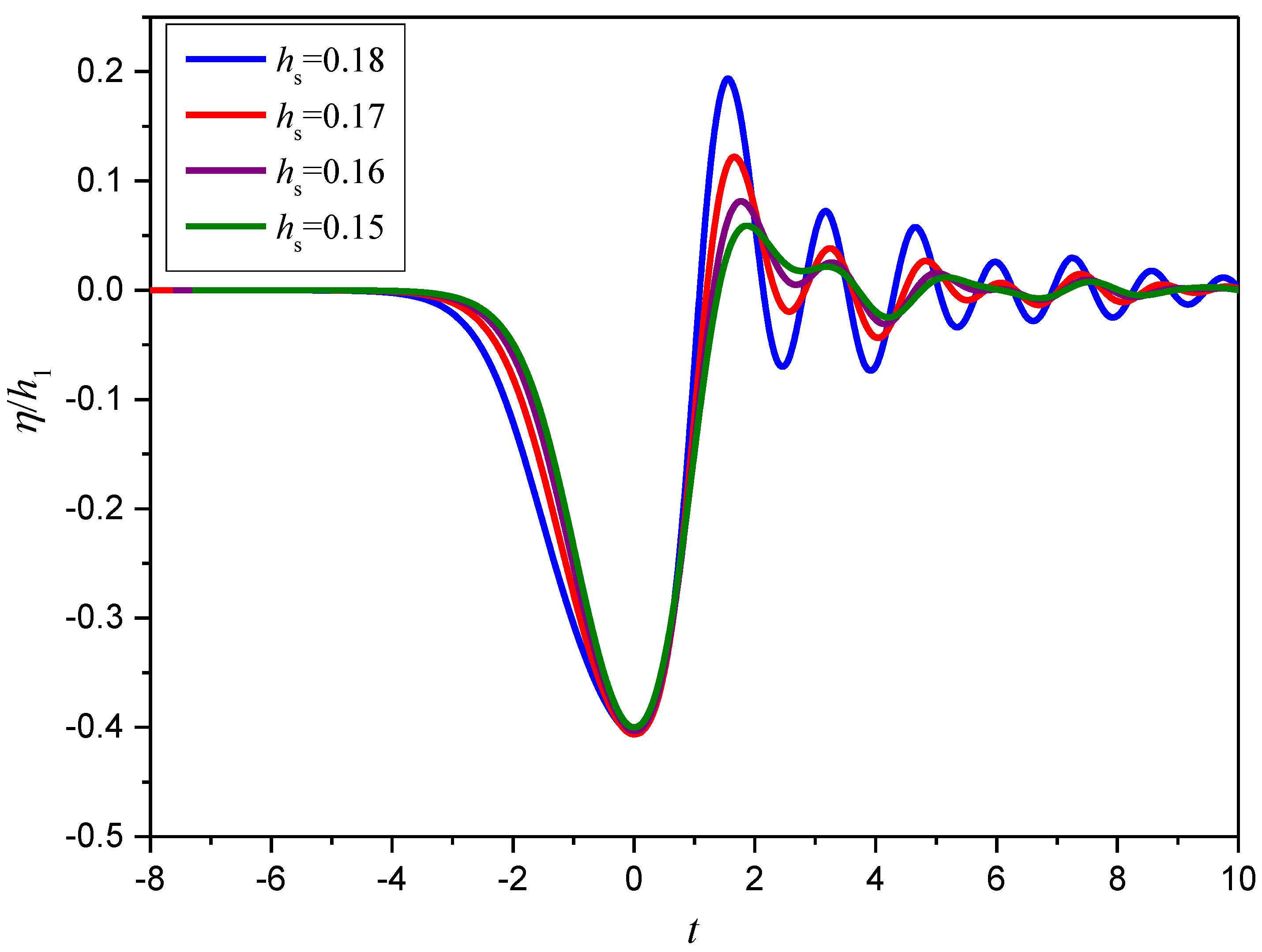
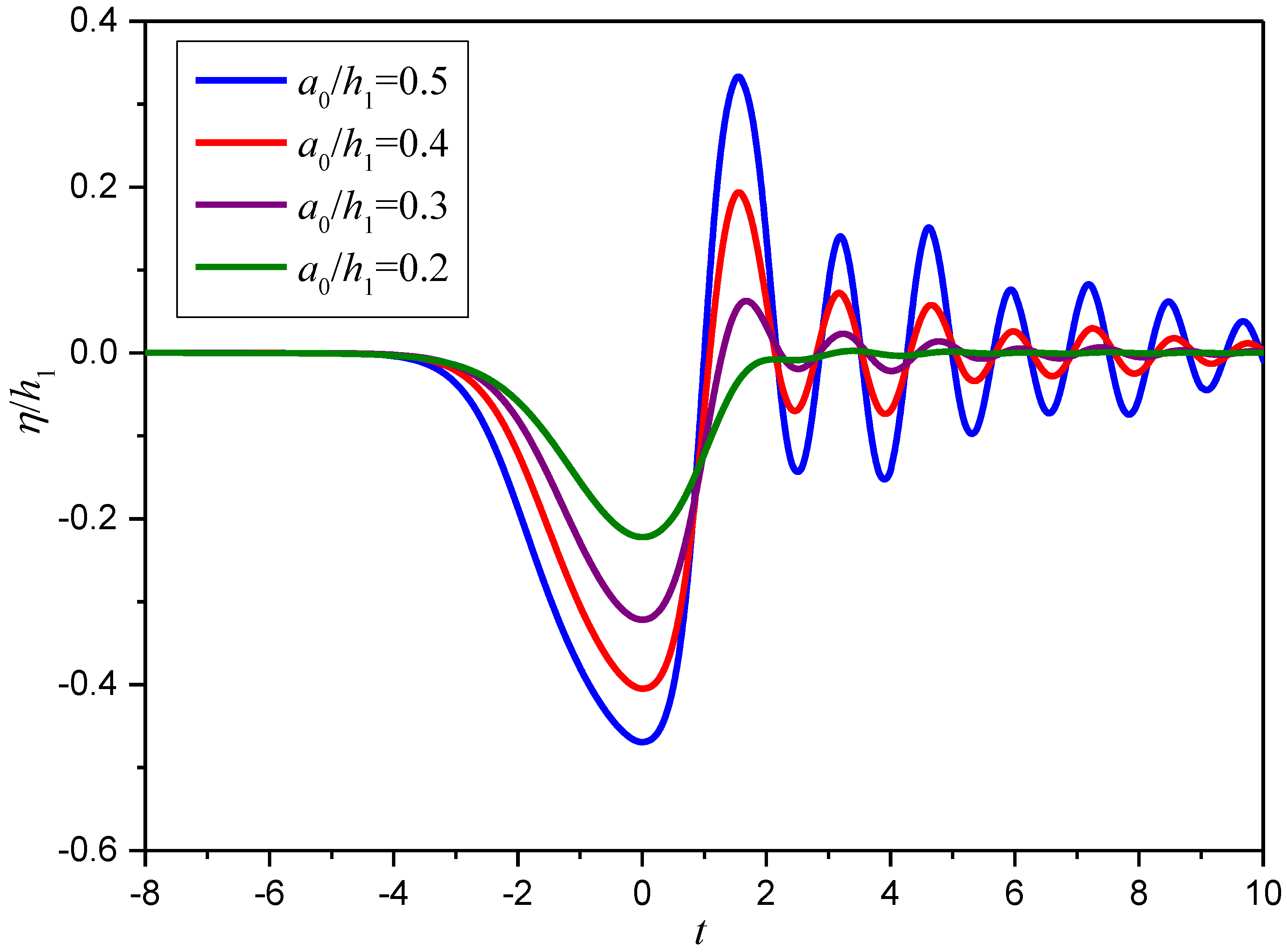
3.3. Tail Waves
4. Conclusions
Author Contributions
Funding
Conflicts of Interest
References
- Helfrich, K.R.; Melville, W.K. Long Nonlinear Internal Waves. Annu. Rev. Fluid Mech. 2006, 38, 395–425. [Google Scholar] [CrossRef]
- Stanton, T.P.; Ostrovsky, L. Observations of highly nonlinear internal solitons over the continental shelf. Geophys. Res. Lett. 1998, 25, 2695–2698. [Google Scholar] [CrossRef]
- Magalhaes, J.M.; Da Silva, J.C.B. Internal Solitary Waves in the Andaman Sea: New Insights from SAR Imagery. Remote Sens. 2018, 10, 861. [Google Scholar] [CrossRef] [Green Version]
- Li, Y.; Wang, C.; Liang, C.; Li, J.; Liu, W. A simple early warning method for large internal solitary waves in the northern South China Sea. Appl. Ocean Res. 2016, 61, 167–174. [Google Scholar] [CrossRef]
- Jia, T.; Liang, J.; Li, X.-M.; Fan, K. Retrieval of Internal Solitary Wave Amplitude in Shallow Water by Tandem Spaceborne SAR. Remote Sens. 2019, 11, 1706. [Google Scholar] [CrossRef] [Green Version]
- Magalhaes, J.M.; Alpers, W.; Santos-Ferreira, A.M.; Da Silva, J.C.B. Surface wave breaking caused by internal solitary waves effects on radar backscattering measured by SAR and radar altimeter. Oceanography 2021, 34, 14–24. [Google Scholar] [CrossRef]
- Ledwell, J.R.; Hickey, B.M. Evidence for enhanced boundary mixing in the Santa Monica Basin. J. Geophys. Res. Space Phys. 1995, 100, 20665–20679. [Google Scholar] [CrossRef]
- Wüest, A.; Piepke, G.; Van Senden, D.C. Turbulent kinetic energy balance as a tool for estimating vertical diffusivity in wind-forced stratified waters. Limnol. Oceanogr. 2000, 45, 1388–1400. [Google Scholar] [CrossRef]
- Aghsaee, P.; Boegman, L.; Lamb, K.G. Breaking of shoaling internal solitary waves. J. Fluid Mech. 2010, 659, 289–317. [Google Scholar] [CrossRef] [Green Version]
- Nakayama, K.; Sato, T.; Shimizu, K.; Boegman, L. Classification of internal solitary wave breaking over a slope. Phys. Rev. Fluids 2019, 4, 014801. [Google Scholar] [CrossRef] [Green Version]
- Tian, Z.; Guo, X.; Qiao, L.; Jia, Y.; Yu, L. Experimental investigation of slope sediment resuspension characteristics and influencing factors beneath the internal solitary wave-breaking process. Bull. Int. Assoc. Eng. Geol. 2017, 78, 959–967. [Google Scholar] [CrossRef]
- Lamb, K.G. Particle transport by nonbreaking, solitary internal waves. J. Geophys. Res. Space Phys. 1997, 102, 18641–18660. [Google Scholar] [CrossRef]
- Cai, S.; Long, X.; Wang, S. Forces and torques exerted by internal solitons in shear flows on cylindrical piles. Appl. Ocean Res. 2008, 30, 72–77. [Google Scholar] [CrossRef]
- Zhu, H.; Lin, C.; Wang, L.; Kao, M.; Tang, H.; Williams, J.J.R. Numerical investigation of internal solitary waves of elevation type propagating on a uniform slope. Phys. Fluids 2018, 30, 116602. [Google Scholar] [CrossRef]
- Lamb, K.G.; Nguyen, V.T. Calculating Energy Flux in Internal Solitary Waves with an Application to Reflectance. J. Phys. Oceanogr. 2009, 39, 559–580. [Google Scholar] [CrossRef]
- Chen, W.; Wang, D.; Xu, L.; Lv, Z.; Wang, Z.; Gao, H. On the Slope Stability of the Submerged Trench of the Immersed Tunnel Subjected to Solitary Wave. J. Mar. Sci. Eng. 2021, 9, 526. [Google Scholar] [CrossRef]
- Li, J.; Zhang, Q.; Chen, T. ISWFoam: A numerical model for internal solitary wave simulation in continuously stratified fluids. Geosci. Model Dev. 2021. preprint. [Google Scholar] [CrossRef]
- Bourgault, D.; Blokhina, M.D.; Mirshak, R.; Kelley, D.E. Evolution of a shoaling internal solitary wave train. Geophys. Res. Lett. 2007, 34, L03601. [Google Scholar] [CrossRef] [Green Version]
- Ali, L.; Makhdoom, N.; Gao, Y.; Fang, P.; Khan, S.; Bai, Y. Metocean Criteria for Internal Solitary Waves Obtained from Numerical Models. Water 2021, 13, 1554. [Google Scholar] [CrossRef]
- Deepwell, D.; Sapède, R.; Buchart, L.; Swaters, G.E.; Sutherland, B.R. Particle transport and resuspension by shoaling internal solitary waves. Phys. Rev. Fluids 2020, 5, 054303. [Google Scholar] [CrossRef]
- Cheng, M.-H.; Hsu, J.R. Effect of frontal slope on waveform evolution of a depression interfacial solitary wave across a trapezoidal obstacle. Ocean Eng. 2013, 59, 164–178. [Google Scholar] [CrossRef]
- Chen, C.-Y.; Hsu, J.R.-C.; Chen, H.-H.; Kuo, C.-F.; Cheng, M.-H. Laboratory observations on internal solitary wave evolution on steep and inverse uniform slopes. Ocean Eng. 2007, 34, 157–170. [Google Scholar] [CrossRef]
- Helfrich, K.R. Internal solitary wave breaking and run-up on a uniform slope. J. Fluid Mech. 1992, 243, 133–154. [Google Scholar] [CrossRef]
- Michallet, H.; Ivey, G.N. Experiments on mixing due to internal solitary waves breaking on uniform slopes. J. Geophys. Res. Space Phys. 1999, 104, 13467–13477. [Google Scholar] [CrossRef]
- Cavaliere, D.; la Forgia, G.; Adduce, C.; Alpers, W.; Martorelli, E.; Falcini, F. Breaking Location of Internal Solitary Waves Over a Sloping Seabed. J. Geophys. Res. Oceans 2021, 126, e2020JC016669. [Google Scholar] [CrossRef]
- Helfrich, K.R.; Melville, W.K.; Miles, J.W. On interfacial solitary waves over slowly varying topography. J. Fluid Mech. 1984, 149, 305–317. [Google Scholar] [CrossRef] [Green Version]
- Orr, M.H.; Mignerey, P.C. Nonlinear internal waves in the South China Sea: Observation of the conversion of depression internal waves to elevation internal waves. J. Geophys. Res. Space Phys. 2003, 108. [Google Scholar] [CrossRef]
- Shroyer, E.L.; Moum, J.N.; Nash, J. Observations of Polarity Reversal in Shoaling Nonlinear Internal Waves. J. Phys. Oceanogr. 2009, 39, 691–701. [Google Scholar] [CrossRef] [Green Version]
- Zhi, C.; Chen, K.; You, Y. Internal solitary wave transformation over the slope: Asymptotic theory and numerical simulation. J. Ocean Eng. Sci. 2018, 3, 83–90. [Google Scholar] [CrossRef]
- Lamb, K.G.; Xiao, W. Internal solitary waves shoaling onto a shelf: Comparisons of weakly-nonlinear and fully nonlinear models for hyperbolic-tangent stratifications. Ocean Model. 2014, 78, 17–34. [Google Scholar] [CrossRef]
- Longuet-Higgins, M.S.; Cokelet, E.D. Deformation of steep surface-waves on water. Proc. R. Soc. A Math. Phys. Eng. Sci. 1976, 350, 1–26. [Google Scholar]
- Liu, P.L.-F.; Hsu, H.-W.; Lean, M.H. Applications of boundary integral equation methods for two-dimensional non-linear water wave problems. Int. J. Numer. Methods Fluids 1992, 15, 1119–1141. [Google Scholar] [CrossRef]
- Sun, Z.; Pang, Y.; Li, H. Two dimensional fully nonlinear numerical wave tank based on the BEM. J. Mar. Sci. Appl. 2012, 11, 437–446. [Google Scholar] [CrossRef]
- Jiang, S.-C.; Teng, B.; Gou, Y.; Ning, D.-Z. A precorrected-FFT higher-order boundary element method for wave–body problems. Eng. Anal. Bound. Elem. 2012, 36, 404–415. [Google Scholar] [CrossRef]
- Riesner, M.; el Moctar, O. A time domain boundary element method for wave added resistance of ships taking into account viscous effects. Ocean Eng. 2018, 162, 290–303. [Google Scholar] [CrossRef]
- Abbasnia, A.; Soares, C.G. Fully nonlinear simulation of wave interaction with a cylindrical wave energy converter in a numerical wave tank. Ocean Eng. 2018, 152, 210–222. [Google Scholar] [CrossRef]
- Grilli, S.T.; Subramanya, R.; Svendsen, I.A.; Veeramony, J. Shoaling of Solitary Waves on Plane Beaches. J. Waterw. Port Coast. Ocean Eng. 1994, 120, 609–628. [Google Scholar] [CrossRef] [Green Version]
- Grilli, S.T.; Svendsen, I.A.; Subramanya, R. Breaking Criterion and Characteristics for Solitary Waves on Slopes. J. Waterw. Port Coast. Ocean Eng. 1997, 123, 102–112. [Google Scholar] [CrossRef] [Green Version]
- Guyenne, P.; Grilli, S.T. Numerical study of three-dimensional overturning waves in shallow water. J. Fluid Mech. 2006, 547, 361–388. [Google Scholar] [CrossRef] [Green Version]
- Koo, W. Free surface simulation of a two-layer fluid by boundary element method. Int. J. Nav. Archit. Ocean Eng. 2010, 2, 127–131. [Google Scholar] [CrossRef] [Green Version]
- Gou, Y.; Chen, X.-J.; Bin, T. A Time-Domain Boundary Element Method for Wave Diffraction in a Two-Layer Fluid. J. Appl. Math. 2012, 2012, 686824. [Google Scholar] [CrossRef]
- Evans, W.A.B.; Ford, M.J. An integral equation approach to internal (2-layer) solitary waves. Phys. Fluids 1996, 8, 2032–2047. [Google Scholar] [CrossRef]
- Gao, X.-W.; Guo, L.; Zhang, C. Three-step multi-domain BEM solver for nonhomogeneous material problems. Eng. Anal. Bound. Elem. 2007, 31, 965–973. [Google Scholar] [CrossRef]
- Zou, L.; Hu, Y.; Wang, Z.; Pei, Y.; Yu, Z. Computational analyses of fully nonlinear interaction of an internal solitary wave and a free surface wave. AIP Adv. 2019, 9, 035234. [Google Scholar] [CrossRef] [Green Version]
- Camassa, R.; Choi, W.; Michallet, H.; Rusås, P.-O.; Sveen, J.K. On the realm of validity of strongly nonlinear asymptotic approximations for internal waves. J. Fluid Mech. 2006, 549, 1–23. [Google Scholar] [CrossRef] [Green Version]
- Kakutani, T.; Yamasaki, N. Solitary Waves on a Two-Layer Fluid. J. Phys. Soc. Jpn. 1978, 45, 674–679. [Google Scholar] [CrossRef]
- Kodaira, T.; Waseda, T.; Miyata, M.; Choi, W. Internal solitary waves in a two-fluid system with a free surface. J. Fluid Mech. 2016, 804, 201–223. [Google Scholar] [CrossRef] [Green Version]
- Grue, J.; Jensen, A.; Rusås, P.-O.; Sveen, J.K. Properties of large-amplitude internal waves. J. Fluid Mech. 1999, 380, 257–278. [Google Scholar] [CrossRef] [Green Version]

| a/h1 | hs | β | h1/h2 | ρ1/ρ2 |
|---|---|---|---|---|
| 0.5 | 0.14~0.18 | 20° | 0.2 | 0.859 |
| 0.4 | 0.14~0.18 | 20° | 0.2 | 0.859 |
| 0.3 | 0.14~0.18 | 20° | 0.2 | 0.859 |
| 0.2 | 0.14~0.18 | 20° | 0.2 | 0.859 |
| 0.4 | 0.18 | 15° | 0.2 | 0.859 |
| 0.4 | 0.18 | 10° | 0.2 | 0.859 |
| 0.4 | 0.18 | 5° | 0.2 | 0.859 |
Publisher’s Note: MDPI stays neutral with regard to jurisdictional claims in published maps and institutional affiliations. |
© 2021 by the authors. Licensee MDPI, Basel, Switzerland. This article is an open access article distributed under the terms and conditions of the Creative Commons Attribution (CC BY) license (https://creativecommons.org/licenses/by/4.0/).
Share and Cite
Hu, Y.; Zou, L.; Ma, X.; Sun, Z.; Wang, A.; Sun, T. Numerical Simulation for the Evolution of Internal Solitary Waves Propagating over Slope Topography. J. Mar. Sci. Eng. 2021, 9, 1224. https://doi.org/10.3390/jmse9111224
Hu Y, Zou L, Ma X, Sun Z, Wang A, Sun T. Numerical Simulation for the Evolution of Internal Solitary Waves Propagating over Slope Topography. Journal of Marine Science and Engineering. 2021; 9(11):1224. https://doi.org/10.3390/jmse9111224
Chicago/Turabian StyleHu, Yingjie, Li Zou, Xinyu Ma, Zhe Sun, Aimin Wang, and Tiezhi Sun. 2021. "Numerical Simulation for the Evolution of Internal Solitary Waves Propagating over Slope Topography" Journal of Marine Science and Engineering 9, no. 11: 1224. https://doi.org/10.3390/jmse9111224
APA StyleHu, Y., Zou, L., Ma, X., Sun, Z., Wang, A., & Sun, T. (2021). Numerical Simulation for the Evolution of Internal Solitary Waves Propagating over Slope Topography. Journal of Marine Science and Engineering, 9(11), 1224. https://doi.org/10.3390/jmse9111224