Article

Atmospheric Emissions in Ports Due to Maritime Traffic in Mexico

by
Gilberto Fuentes García
1,*,
Rodolfo Sosa Echeverría
1,
José María Baldasano Recio
2,3,
Jonathan D. W. Kahl
4,
Elías Granados Hernández
5,
Ana Luisa Alarcón Jímenez
1 and
Rafael Esteban Antonio Durán
6
1
Sección de Contaminación Ambiental, Ciudad Universitaria, Instituto de Ciencias de la Atmósfera y Cambio Climático, Universidad Nacional Autónoma de México, Mexico City 04510, Mexico
2
Barcelona Supercomputing Center-Centro Nacional de Supercomputación (BSC-CNS), Department of Earth Sciences, Nexus II Building, Jordi Girona 29, 08034 Barcelona, Spain
3
Department of Engineering Design, Universitat Politècnica de Catalunya (UPC), Av. Diagonal 647, Planta 10, 08028 Barcelona, Spain
4
School of Freshwater Science, University of Wisconsin-Milwaukee, Milwaukee, WI 53201, USA
5
Centro Tecnológico FES-Aragón, Laboratorio Ambiental, Universidad Nacional Autónoma de México, Nezahualcoyotl 57130, Mexico
6
Facultad de Ingeniería, Ciudad Universitaria, Universidad Nacional Autónoma de México, Mexico City 04510, Mexico
*
Author to whom correspondence should be addressed.
J. Mar. Sci. Eng. 2021, 9(11), 1186; https://doi.org/10.3390/jmse9111186
Submission received: 8 October 2021 / Revised: 22 October 2021 / Accepted: 23 October 2021 / Published: 27 October 2021
(This article belongs to the Section Marine Pollution)

Abstract

:
Atmospheric emissions from vessels at 38 Pacific and Gulf-Caribbean Mexican ports were determined for nitrogen oxides, sulfur dioxide, particulates, carbon monoxide, non-methane volatile organic compounds, and carbon dioxide. The emissions have been estimated using a bottom-up methodology in the maneuver and hoteling phases, by vessel type, from 2005 to 2020. Maritime traffic in Mexico’s Pacific zone contributes approximately with 60% of the country’s total ship emissions, with the remaining 40% in Gulf-Caribbean ports. The highest atmospheric emissions were found at the Manzanillo and Lázaro Cárdenas ports on the Pacific coast, as well as the Altamira and Veracruz ports on the Gulf-Caribbean coast. The contribution of the atmospheric emissions by vessel type at Pacific ports was Container 67%, Bulk Carrier 32%, Tanker 0.8%, and RoRo 0.4%. For Gulf-Caribbean ports it was Container 76%, Bulk Carrier 19%, Tanker 3%, and RoRo 2%. This study incorporates the International Maritime Organization implementations on reductions of sulfur content in marine fuel, from 4.5% mass by mass from 2005 to 2011, to 3.5% from 2012 to 2019, to 0.5% beginning in 2020. Overall, sulfur dioxide emissions were reduced by 89%.

1. Introduction

In 1973 the International Maritime Organization (IMO) adopted the Marine Pollution Convention (MARPOL 73/78). The Convention considers regulations to prevent and minimize pollution from ships and accidental pollution from routine operations in the marine environment according to six technical Annexes. The agreement was entered into force in 1983, with a 1997 amendment (Annex VI) adopted in 2008 and entered into force in 2010. The agreement caused a significant reduction in sulfur oxides (SOx) and nitrogen oxides (NOx) emissions from marine engines [1]. Likewise, new amendments adopted in 2011 and entered into force in 2013 established mandatory measures to reduce greenhouse gas emissions from international maritime transport. The reduction of sulfur content in fuel oil, from 4.5% mass by mass (m/m) before 2000 to 31 December 2011, 3.5% m/m in 2012 to 31 December 2019, and 0.5% m/m in 2020, will allow a considerable additional reduction of sulfur oxides from vessels, improve air quality in port cities and coastal areas, and meet global goals in the fight against climate change [2,3,4,5]. Four established emission control areas (ECAs) already have stricter regulations: Baltic Sea, North Sea, North American, and United States Caribbean Sea. In effect since 2015, within the control areas, the sulfur oxide emissions limit is 0.10% m/m. This will not change with IMO 2020 regulations.
International maritime transport accounts for approximately 80% of global freight between peoples and communities around the world [2,3,4]. It is a safe, efficient, and profitable international transport system for most goods, and fosters trade between nations and peoples, while contributing to their prosperity. The world depends on a safe, secure, and efficient international shipping industry, which is achieved through the regulatory framework that is established and kept up to date within the IMO.
International maritime trade is forecast to expand at an average annual rate of 2.6% in 2019 and 3.4% in the period 2019–2024, driven mainly by an increase in Container, Bulk Carrier, and Liquid-gas ships [2]. In 2018, ships spent an average of 23.5 h in port (specifically, 2.05 days for bulk carriers and 0.7 days for container ships) by [2]. The typical spent time in port for a ship calling was 0.97 days [6] and [7]. The short time in port is a positive indicator of the efficiency level and commercial competitiveness of a port. The countries with the longest stay times in port correspond mainly to developing countries or the least developed countries [2]. In total, 64% of container port traffic occurs in Asia, followed by Europe (16%), North America (8%), Latin America and the Caribbean (7%), Africa (4%), and Oceania (2%). These percentages largely reflect the level of participation of different countries in global movement of merchandise, with containerized cargo increasing in importance due to its average annual growth rate of 8% between 1980 and 2018 [2].
Given these considerations, that exist at the international level, we have determined the level of atmospheric emission due to the port system in Mexico for the Pacific and Gulf-Caribbean, considering the movement of vessels in ports in the maneuvering and hoteling phases from 2005 to 2020. Considering the provisions of the IMO and MARPOL 73/78, atmospheric emissions of NOx, sulfur dioxide (SO2), particulates (PM), carbon monoxide (CO), non-methane volatile organic compounds (NMVOC), and carbon dioxide (CO2) were determined using the “bottom-up” method [8]. This method requires information on technical operating characteristics, time spent in maneuvering and hoteling phases, power, and load factor of the main (ME) and auxiliary (AE) engines, specific fuel consumption (sfc), and emission factors for each phase of navigation. All such information, as well as details of ship and cargo type, is reported by the “Secretaría de Comunicaciones y Transportes” (SCT) [9], the controlling body of the port system in Mexico.
Currently, the issue of atmospheric emissions from the port sector in Mexico is not considered a priority activity, although Mexico is a member of the IMO and MARPOL 73/78. Therefore, the contribution of this study is fundamental at the international level because it is a starting point for the development of other studies that are necessary in Mexico. The main objective of our study was to identify the temporal variability of atmospheric emissions due to the movement of ships since 2005 considering the implementations and regulations of the IMO respect to the change of the sulfur content in marine fuel, that is, in accordance with the IMO in its MARPOL Agreement, Annex VI, SO2 emissions by vessel corresponding to a progression of sulfur contents of 4.5%, 3.5%, and 0.5% m/m, from 2005 to 2020. This allowed us to identify the level of reduction in atmospheric emissions from SO2 assuming that fossil fuels will continue to be used in the coming years within the maritime sector. The results of this study will provide a motivation to monitor and model air quality in coastal zones, and activities that are not carried out in Mexico and are not of priority.
Considering the progress of the methods for estimating atmospheric emissions due to the movement of ships in port, the Automatic Identification System is used to identify the level of atmospheric emission considering algorithms for it. However, the Automatic Identification System is confidential in Mexico and there are restrictions on its use, therefore, this is a limitation of our study. Given this consideration, we use the current official information from the literature that exists at the international level regarding emission factors, time spent in maneuvering and hoteling phases of vessels to determine atmospheric emissions. Due to the current implementation of IMO, it was a great opportunity to evaluate the trend of atmospheric emissions by SO2 in Mexico because there were three scenarios to identify the level of reduction of this specific pollutant. This study clearly reflects the situation currently in Mexico respect to the level of atmospheric emissions from ships for 15 years, and according to Fuentes et al. [10] it is necessary to consider other system ports in Mexico to identify the level of atmospheric emission for main pollutants emitted from ship activities on Pacific and Gulf of Mexico because there is no information about it, and the issue of atmospheric emissions from ships should be a priority in Mexico due to fossil fuels being in use in the future for maritime sectors.

2. Background

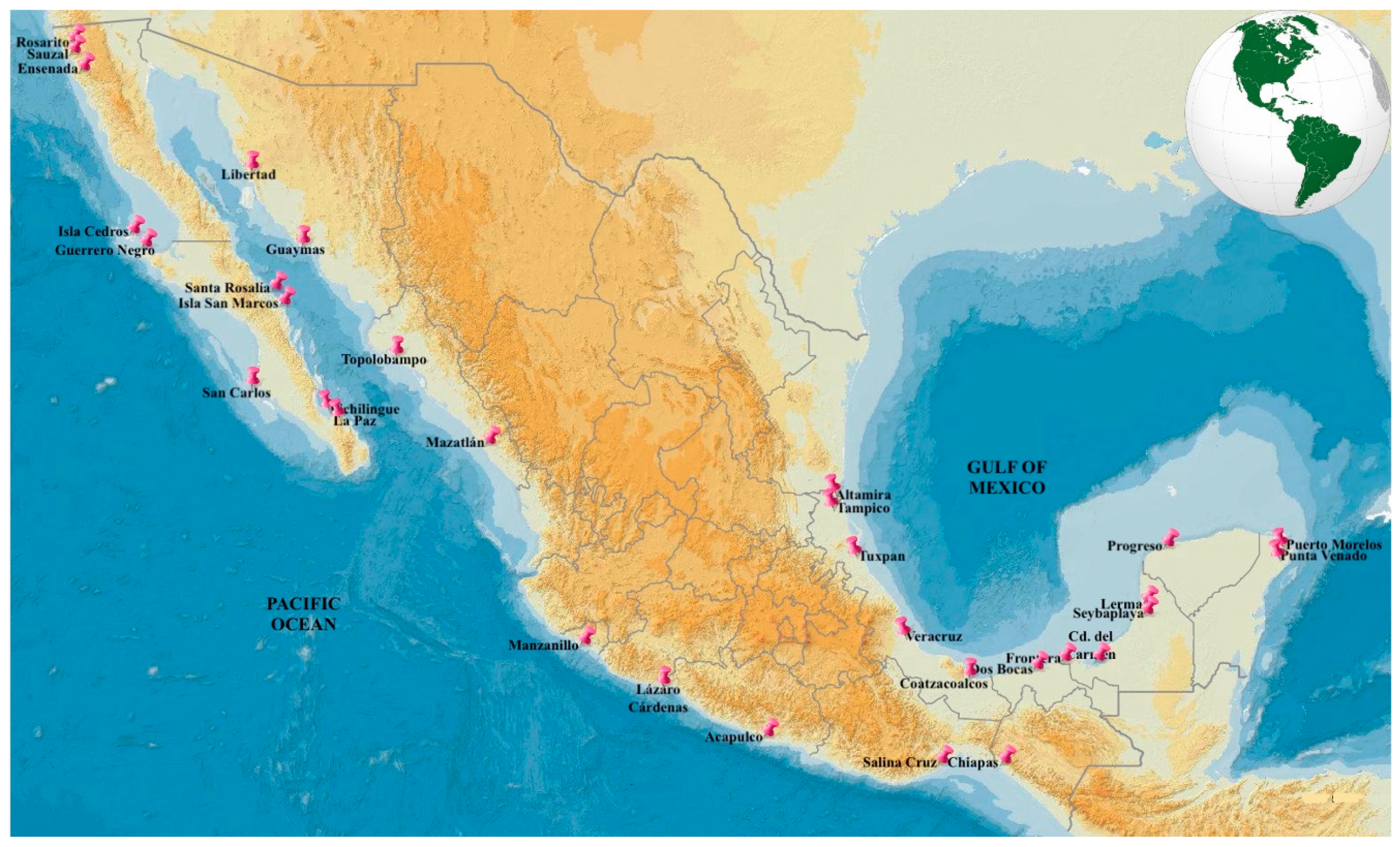
2.1. Port System in Mexico

In Mexico, maritime activity is very important because exports have increased in recent years, and a third of the merchandise that moves from Mexico is by sea. The need to understand the level of atmospheric pollution from port activity in Mexico is thus a relevant issue, especially since some national ports are undergoing maritime development and expansion. To date, few studies have addressed the issue of atmospheric pollution emissions from port activities in Mexico. Fuentes et al. [10] determined the level of atmospheric emissions for main pollutants due to the movement of ships in maneuver and hoteling positions using the bottom-up method, this is the first study carried out in Mexico to characterize one of the most important ports located in the Gulf of México, port of Veracruz. Emissions from maritime vessels in Mexico have an important influence on air quality in coastal areas and, in some cases, inland air quality [11]. The most important pollutants emitted by ships are CO2, NOx, SOx, CO, hydrocarbons (HC), and PM. These are harmful air pollutants that impact air quality, human health, and climate on local, regional, and global scales. Mexico is currently updating its National Inventory of Greenhouse Gas and Compound Emissions, as part of its commitment to the United Nations Framework Convention on Climate Change [12]. Mexico is responsible for preparing, periodically updating, publishing, and facilitating the national inventories of anthropogenic emissions due to different emission sources [13]. The “Instituto Nacional de Ecología y Cambio Climático” (INECC) prepares and updates the inventory of anthropogenic emissions, including emission estimates from the burning of fossil fuels. The methods for estimating anthropogenic emissions are based on the scientific and technical criteria established by the Intergovernmental Panel on Climate Change [14]. Mobile, non-highway transport sources contribute 26.2% of the total emissions nationwide [15,16]. However, there is no detailed information on shipping emissions. Our study thus contributes detailed, nationwide information on anthropogenic emissions for the port sector.
The National Port System handled 267 million tons of cargo in 2020, 12% less than in 2019. Liquids and derivates represented 39.7% of the national total cargo, Bulk Mineral 22.5%, Container 17.8%, General Cargo 9.1%, Bulk Agricultural 6.3%, and Fluids 4.6%. Container traffic handled 6.5 millions of Twenty-foot Equivalent Unit (TEU), 9.1% less than in January to December 2019 [17].
The ports considered in this study are shown in Figure 1. We considered the ports included in the Monthly Statistical Report issued by SCT [9]: 22 ports in the Pacific and 16 in the Gulf-Caribbean. The ports have a Federal-SCT classification that corresponds to “Administración Portuaria Integral” (API), the most important in Mexico.
In 2020 a total of 7245 vessels were served in the Pacific, and 13,999 in the Gulf-Caribbean, with a total of 21,244 vessels served. With this level of vessel activity, it is necessary to understand the atmospheric emission levels generated by port activity on the Pacific and Gulf-Caribbean coasts.
A summary of vessels and cargo type arriving at Pacific and Gulf-Caribbean ports for 2020 is shown in Table 1. The main commercial ports of Mexico, based on the influx of vessels, are Mazatlán, Manzanillo, and Lázaro Cárdenas (Pacific) and Altamira, Veracruz, Coatzacoalcos, Dos Bocas, and Carmen (Gulf-Caribbean). Most of the vessels served in Pacific ports were Container and Bulk Carrier, while RoRo and Tanker vessels were the most frequent in Gulf-Caribbean ports. The port of Manzanillo registered a total of 1256 container vessels served, while the port of Altamira and Veracruz together served 1177 vessels, indicating that the port of Manzanillo is the main port for the movement of Container cargo on the Pacific. On the Gulf-Caribbean, the ports of Dos Bocas and Carmen are principal in the movement of loose general cargo.

2.2. Methods for Estimating Atmospheric Emissions

Currently, there are two methods for estimating atmospheric emissions due to the combustion process carried out in the ME and AE of the ship in the navigation phases of cruising, maneuvering and hoteling. The first is based on fuel consumption [18] and is called top-down. The parameters required for its use correspond to the Gross Tonnage (GT) as a function of ship type and marine fuel consumption. Trozzi and Vaccaro [18] developed an expression to determine the ship fuel consumption based on GT and ship type. The emission factors for this method are based on engine type: steam turbine (ST), high speed diesel (HSD), medium speed diesel (MSD), slow speed diesel (SSD), and gas turbine (GTu), and are available for the atmospheric pollutants NOx, CO, CO2, volatile organic compounds (VOC), PM, and SO2. Trozzi and Vaccaro [19] presented an adjustment to their top-down methodology and considered future scenarios for estimating atmospheric emissions.
The second method is called bottom-up and is the most widely used method for estimating atmospheric emissions from ships because detailed information about the fuel consumption by vessel type is often lacking. The bottom-up method considers the technical aspects of the vessel: (1) type of vessel, (2) GT, (3) power of the ME and AE, (4) load factor of the ME and AE, (5) time spent by the vessel in cruise, maneuver, and hoteling phases, and (6) emission factor [6,8,20], Cooper and Gustafsson [21,22,23,24]. The power of the ME and AE depend on the GT for each type of ship. Atmospheric emissions are determined for the three ship navigation phases for both the ME and AE. Consideration of engine type makes the method more specific, with emission factors corresponding to many pollutants including criteria pollutants, organic and inorganic toxics, and greenhouse gases [6,8], according to Cooper and Gustafsson [21]. Currently, there are studies related to identifying the problems in the time spent in the maneuver and hoteling position by ships. Specifically, in the speed reduce zone in ports. Those considerations are very important due to the level of atmospheric emissions depends on these factors. Venturini et al. [25] used the Berth Allocation Problem (BAP) to optimize problem in hoteling times and position to ships in container terminals because the problem consisted for determining arrival times, berthing times, and berthing positions for each vessel for each port in the string where the handling time for each vessel is known for each port-berth combination. They found a reduction of atmospheric emission up to 42% applying the BAP method. Zhang et al. [26] identified the cold chain mode choice selection with five additional considerations, namely, optimal shipment scheduling, two different bulk ship deployment methods, reefer bulk ship speed optimization, time dependent cargo depreciation, and atmospheric emissions (greenhouse gases only) considering the container and bulk cargo. Findings from a numerical example show that optimal ship speed decreases with a reducing rate when the bunker price increases and with a higher decline rate when goods are less perishable. They considered two models to select between chartered reefer fleet deployment methods and to decide the optimal operation of the reefer bulk fleet.
The Ship Traffic Emissions Assessment Model (STEAM) is a method used by various port systems to estimate atmospheric emissions arising from the combustion process of engines (ME and AE) within different ships and navigation phases. The model relies on information generated by in real time by the Automatic Identification System (AIS) (ship-port). The AIS is useful for the evaluation of ship emissions, as it provides continuous automatic information on the vessel positions and instantaneous speeds of ships. If the required vessel characteristics are also known, the exhaust emissions can be modelled at very high temporal and spatial resolution. Both the geographical coverage achieved via AIS satellite receivers, and the amount of usable AIS-based shipping activity data have substantially increased while the financial costs for acquiring the relevant AIS data have significantly decreased. The availability of the new data has made it possible to use refined methods that can significantly improve the quality of bottom-up ship emission inventories, Johansson et al. [27]. The AIS messages provide data which increase the precision of atmospheric emissions estimates, with minimal uncertainty, as shown by Jalkanen et al. [28,29]. Separate emission factors for NOx, PM, SOx, CO2, and CO are used in the STEAM model [28,29,30]. For example, the NOx emission factor is estimated by the rotation data of the motor shaft [28]. The emission factors change according to the engine load and can be higher for engines that operate at low loads. This is particularly true during maneuvers in port [29]. A recent model validation study showed the best performance when ship speed is 70–75% of service speed. With decreased or increased speed, the model tends to diverge from real-world observations. The model also provides a proxy for the calculation of fuel consumption [31]. Due to the increase in the ships data availability and particularly following the introduction of the AIS, bottom-up studies are nowadays generally more popular than top-down, as shown by Toscano and Murena [32]. In Zhang et al. [33] the use of AIS for Singapore port consisted in a tangible analytical approach to analyze ship traffic demand and the spatial–temporal dynamics of ship traffic in port considering 182 million records in this port were used to assess the developed approach. The proposed approach includes the two modules: traffic demand analysis module, and traffic state spatial –temporal analysis module. Additionally, Zhang et al. [33] investigated the spatial distribution of ship speed and ship accidents using the field data. It was found that hotspot areas of speed were also hotspot areas of ship accidents. Nevertheless, ship density showed no significant relationship with ship accidents. However, the situation of Mexico regarding the use of AIS to characterize the port system in the Pacific and Gulf-Caribbean is not currently viable because this type of information is confidential and there are many restrictions on its use.
These details are relevant to the inclusion of ship emissions while in port in national emission inventories. Browning and Bailey [34] indicate that to develop an atmospheric emissions inventory, a three-tiered approach should be utilized: (1) a quantification of each ship’s trip into and out of a port, along with estimates of harbor craft and land-side emissions; (2) a mid-tier approach where ship trips are averaged by vessel type and dead weight tonnage, allowing the calculation of average trip characteristics; and (3) a streamlined approach in which marine, harbor craft, and land-side emissions are estimated from other detailed inventories. However, we believe that there are other considerations relevant to the development of an atmospheric emissions inventory: fuel consumption by vessel type, sulfur content in the fuel, port location, power changes in the ME and AE, time spent in the maneuvering and hoteling positions, method selected to estimate the emissions, and detailed vessel information. Browning and Bailey [34] further recommend that the bottom-up method is the most suitable for calculating atmospheric emissions when detailed information on ships is known. Dalsoren et al. [35] indicate that a reliable, up-to-date ship emission inventory is essential for atmospheric scientists quantifying the impact of shipping and for policy makers implementing regulations and incentives for emission reduction and can show where emission reductions can be applied to minimize impacts most effectively. Gutiérrez et al. [36] compared nine inventory methodologies to calculate energy consumption and associated emissions of ships passing through the Strait of Gibraltar. They found acceptable differences of approximately 20% among the methods considered [6], as shown by Jalkanen et al. [28], Hulskotte and Van der Gon [37,38], Corbett and Koehler [39], Eyring et al. [40]. Such emissions can be confidently estimated by available methodologies.
Ship emissions estimates using the bottom-up method have been reported for several locations. De Melo Rodríguez et al. [41] determined the atmospheric emissions of CO2, NOx, SOx, and PM for the port of Barcelona using the bottom-up method, relying on the AIS. They reported that the total emissions derived from 30 cruise vessels amounted to 41,750 tons of CO2, 955 tons of NOx, 900 tons of SOx, and 94 tons of PM. The average emissions estimate per vessel call was 80 tons of CO2, 1.85 tons of NOx, 1.75 tons of SOx, and 0.20 tons of PM. Zhang et al. [42] also determined the atmospheric emissions of SOx, NOx, particulates smaller than 10 micrometers (10µm) (PM10), particulates smaller than 2.5 µm (PM2.5), CO and HC through the bottom-up method and the AIS System in China, and reported that near urban zones, ship emissions of SOx were highest with respect to other pollutants.
Carletti et al. [43] estimated PM10 emissions in the maneuvering and hoteling phase using the bottom-up method and the information available from the EMEP/EEA, assuming a fuel sulfur content of 0.1%. Gutiérrez et al. [44] determined the atmospheric emissions of SO2, NOx, CO2 and PM10 using two bottom-up methods differing by emission factor used and found differences of 16% for NOx and 23% for CO2 among the two methods.
Atmospheric emissions estimated for the navigation phases of each vessel type are determined separately for criteria pollutants (SO2, PM and CO), non-criteria pollutants (NOx), toxic organic compounds (VOC and NMVOC), toxic inorganic compounds as lead (Pb), cadmium (Cd), mercury (Hg), arsenic (As), chromium (Cr), cupper (Cu), nickel (Ni), selenium (Se) and zinc (Zn), and greenhouse gases as CO2, methane (CH4), and nitrous oxide (N2O). All such estimates have an uncertainty associated with the mode of navigation. Cooper and Gustafsson [21] indicate that the atmospheric emissions in the hoteling phase contain uncertainties of 10 to 30% for criteria pollutants and organic toxics, 50% for inorganic toxics, and 20 to 50% for greenhouse gases. In another study, uncertainties of 20 to 40% in the hoteling phase, and 30 to 50% and 10 to 25% in the cruise and maneuvering phases, respectively, were reported [6].
Around 15% of the global anthropogenic NOx and 58% of global SOx emissions are attributable to oceangoing ships, as shown by Eyring et al. [40] and Corbett et al. [45]. The shipping sector is projected to grow by 50–250% by 2050 [46]. Global use of heavy oil and diesel for ships makes a small contribution to climate change of 2.2% of global emissions of CO2 on the order of 795–938 Mt CO2 in 2012 [46]. A more recent model suggests emissions of 831 Mt CO2 in 2015, as shown by Johansson et al. [27]. Given these considerations, Styhre et al. [47] determined the level of greenhouse gas emissions for four ports: port of Gothenburg (150,000-ton CO2), port of Long Beach (240,000-ton CO2), port of Osaka (97,000-ton CO2) and port of Sidney (95,000-ton CO2) considering five navigation phases. The method utilized by Styhre et al. [47] corresponded with bottom-up and AIS, and some parameters of ships from [6] and [21]. According to Styhre et al. [47] this is the first study to compare the greenhouse gas emissions considering different continents. Considering to the provisions by Intergovernmental Panel on Climate Change to reduce the CO2 atmospheric emissions by 2050, Iris and Lam [48] indicate that emission reduction is a direct consequence of the energy efficiency, electrification of equipment, the use of alternative fuels and renewable energy sources, and technological advances also contribute to the fuel consumption efficiency. Recently, energy-aware studies gain attention in automated container terminals. Iris and Lam [48] suggested various techniques to reduce the greenhouse gas emissions: cold-ironing, electrification and technologies for equipment, energy supply, and clean fuels, mainly. However, these technologies are widely used in ports located in developed countries, that is, their political, economic, and environmental level has allowed them to use these methods to reduce the level of atmospheric emissions as well as to develop methods to reduce the greenhouse gas emissions.

2.3. Determining Atmospheric Emissions in Port
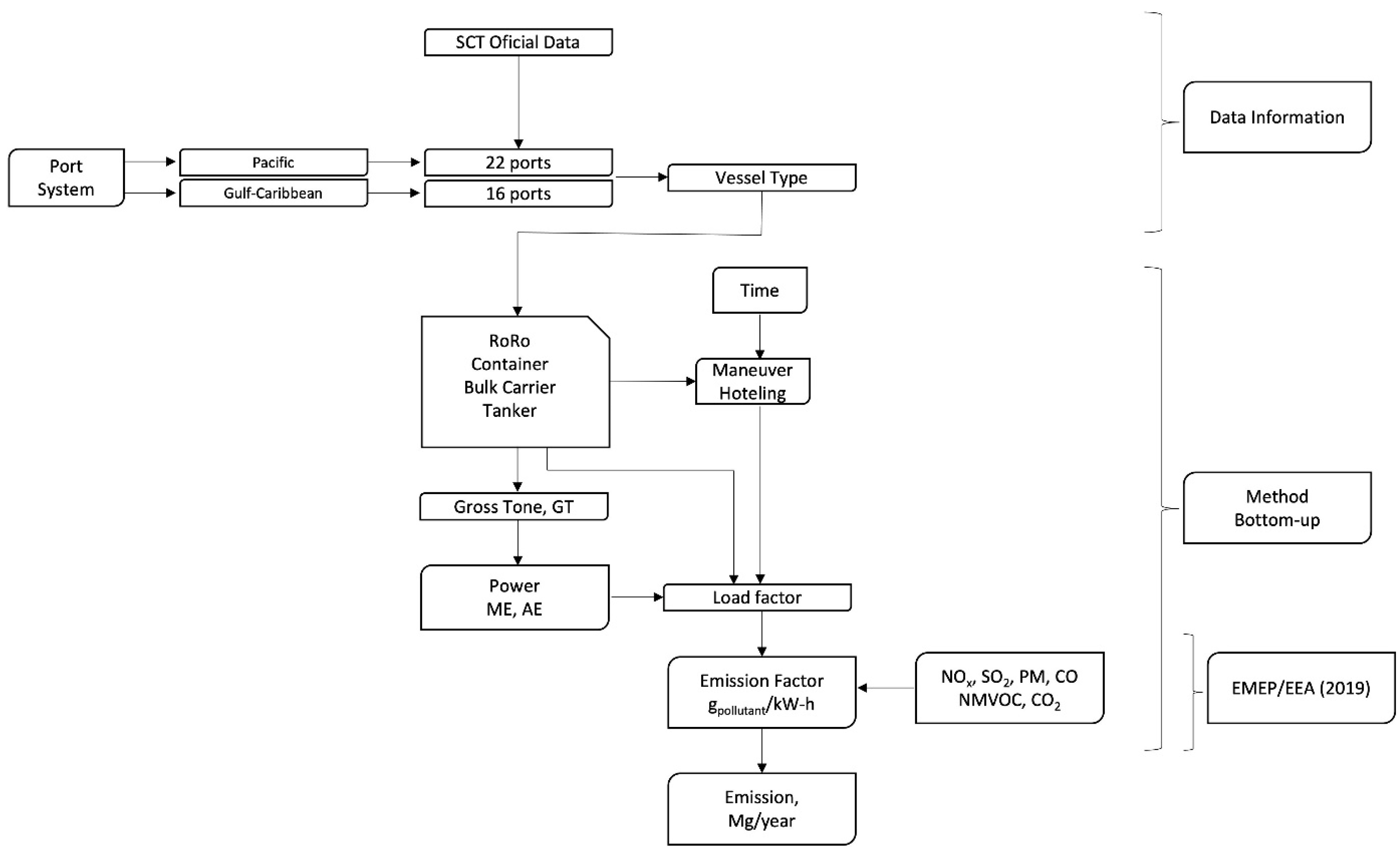
Currently, the approach to determining atmospheric emissions using the bottom-up method is based on ship movement in port, specifically during the maneuvering and hoteling phases [49], as discussed by Knezevic et al. [50] and Cullinane et al. [51]. Toscano and Murena [32] indicate that methodologies for the assessment of ship emissions goes from: full top-down approach to full bottom-up approach. In the full top-down approach total emissions are calculated at a large scale, generally national, and then geographically reduced at a smaller scale (regional or urban) using proxy variables. In the full bottom-up approach, air pollutants emitted by each ship in its specific position and during a specific activity is estimated. Then data are aggregated over the time and the space. Bottom-up methods estimate the emission rates during each specific activity (hoteling, maneuvering and navigation) as the product of an emission factor (EF) multiplied by the energy output of the engine or the fuel consumption. Energy output is generally estimated using the maximum continuous rating engine power multiplied by a load factor. Hulskotte and Van der Gon [37] indicate that over the past decade, expanding international trade has resulted in corresponding rapid growth in the tonnage of goods shipped by sea. Ships are clearly recognized as a major source of air pollution and associated climate change, global warming, acidification, and eutrophication, all of which can have significant adverse effects on human health, as indicated by Yang et al. [52], Deniz and Durmusoglu [53,54], Gibbs et al. [55] and McArthur and Osland [56]. Atmospheric emissions of pollutants such as CO, PM10, PM2.5, VOC, NOx, and SO2 exert deleterious local effects in coastal cities, in the form of environmental and health problems [57]. Emissions from ships in hoteling phase are the fundamental determinants of the concentration of exhaust emissions in ports: NOx 90.1%, PM2.5 78.0%, and SOx 88.5%, shown by [54], Deniz and Civkaroglu [58], and Papaefthimiou et al. [59]. Given the serious health effects of local concentrations of certain ship emissions, there is clearly a case for a focused analysis of ship emissions in the hoteling phase. Of particular importance to human health in urbanized ports, around 95% of the ship-generated total PM emissions are PM2.5 [60].
Some countries monitor the air quality of their port systems, focusing on criteria pollutants [61,62,63,64]. Studies indicate an adverse health effect to the population near a port, including severe impacts on health and the environment, especially in territorial waters, inland seas, canals, straits, bays, and port regions, as discussed by Saracoglu et al. [65]. Based on fuel consumption, the annual CO2, NOx, and SOx emissions from ships constitutes about 2%, 11%, and 4% of global anthropogenic emissions, respectively [66]. On average across Europe, shipping emissions expose 8% of the population to primary PM2.5, 16.5% to NOx, and 11% to SOx. Less than 1% of the population was exposed to shipping emissions of CO, NMVOC and ammonia (NH3) [67].
The need to identify atmospheric emissions from the maneuvering and hoteling phase of vessels in port has thus become, as established by the MARPOL Annex VI agreement, MARPOL 73/78, an essential task that each port must fulfill as a priority activity to protect the health of the general population.
According to the IMO, reducing the sulfur content in fuels from the 2012 level of 2.5% m/m to 0.5% by 2020 will substantially reduce atmospheric emissions of SO2 [3,4,5]. This measure was adopted on 1 January 2020, therefore, the type of ships that currently move around the world will have to use cleaner fuels [7,68]. Speciation analyses of these cleaner fuels will be necessary to determine their impact on ship emissions.

3. Methodology

The procedure for estimating atmospheric emissions of NOx, SO2, PM, CO, NMVOC, and CO2 on an annual basis is shown in Figure 2. The bottom-up method was used, thus incorporating information on typology and vessel details for the different navigation positions as well as differential emission factors for the ME and AE by vessel type for each navigation position. Information about maritime traffic in the port sector in Mexico from 2005 to 2020 was considered [9].
The expression to determine the total emission (maneuvering and hoteling phases) is shown in Equation (1). This method corresponds to [7,8], and Cooper and Gustafsson [21,22,24].
E T = E m a n e u v e r i n g + E h o t e l l i n g  
E T = t m a n e u v e r i n g P M E L F M E E F M E + P A E L F A E E F A E + t h o t e l l i n g P A E L F A E E F A E
where: E T : total Emissions (g), E m a n e u v e r i n g : maneuvering emission (g), E h o t e l l i n g : hoteling emission (g), t m a n e u v e r i n g : time spent in maneuvering phase (h), t h o t e l l i n g : time spent in hoteling phase (h), P M E : power of the ME (kW), P A E : power of the AE (kW), L F M E : load factor of the ME for each navigation phase, L F A E : load factor of the AE for each navigation phase, E F M E : emission factor of the ME for each navigation phase (g/kW), E F A E : emission factor of the AE for each navigation phase (g/kW).
To determine the atmospheric emission by vessel type it is necessary to calculate the power installed for the ME and AE. The power installed for the ME depends on the GT value for each vessel type. These expressions are shown in Table 2, along with the GT average and the number of samples by ship type [7,69]. The power of AE by vessel type is determined by multiplying the power of ME by the ratio AE/ME.
The load factor used for the emission calculation was 20% for all vessels except for the Tanker vessel. For Tanker vessels a load factor of 40% was used in the hoteling phase for the AE according to [6], Cooper and Gustafsson [21]. Nicewicz and Tarnapowicz [70] also provide load factor data in the hoteling phase by type of vessel as well as the power of the ME and AE. For the maneuvering phase, 20% was considered as the load factor for the ME and 50% for the AE for all vessels in accordance with [6].
The emission factors considered in this study are shown in Table 3 and correspond to reported values [8] for all pollutants except CO2. As the CO2 emission factor is not reported by [8] the one reported by [7,22] was used. SO2 emission factors are based on the IMO regulation periods and Sulphur content in marine fuel.
The spent time in the maneuvering and hoteling phase by type of vessel is an important factor that must be considered in the estimation of atmospheric emissions from vessels. Most of the time, the AE is operating in the hoteling position, while both the ME and AE work in the maneuvering position. Table 4 shows the time spent in the maneuvering and hoteling stage for each vessel in operation [6,71].

4. Results and Discussion

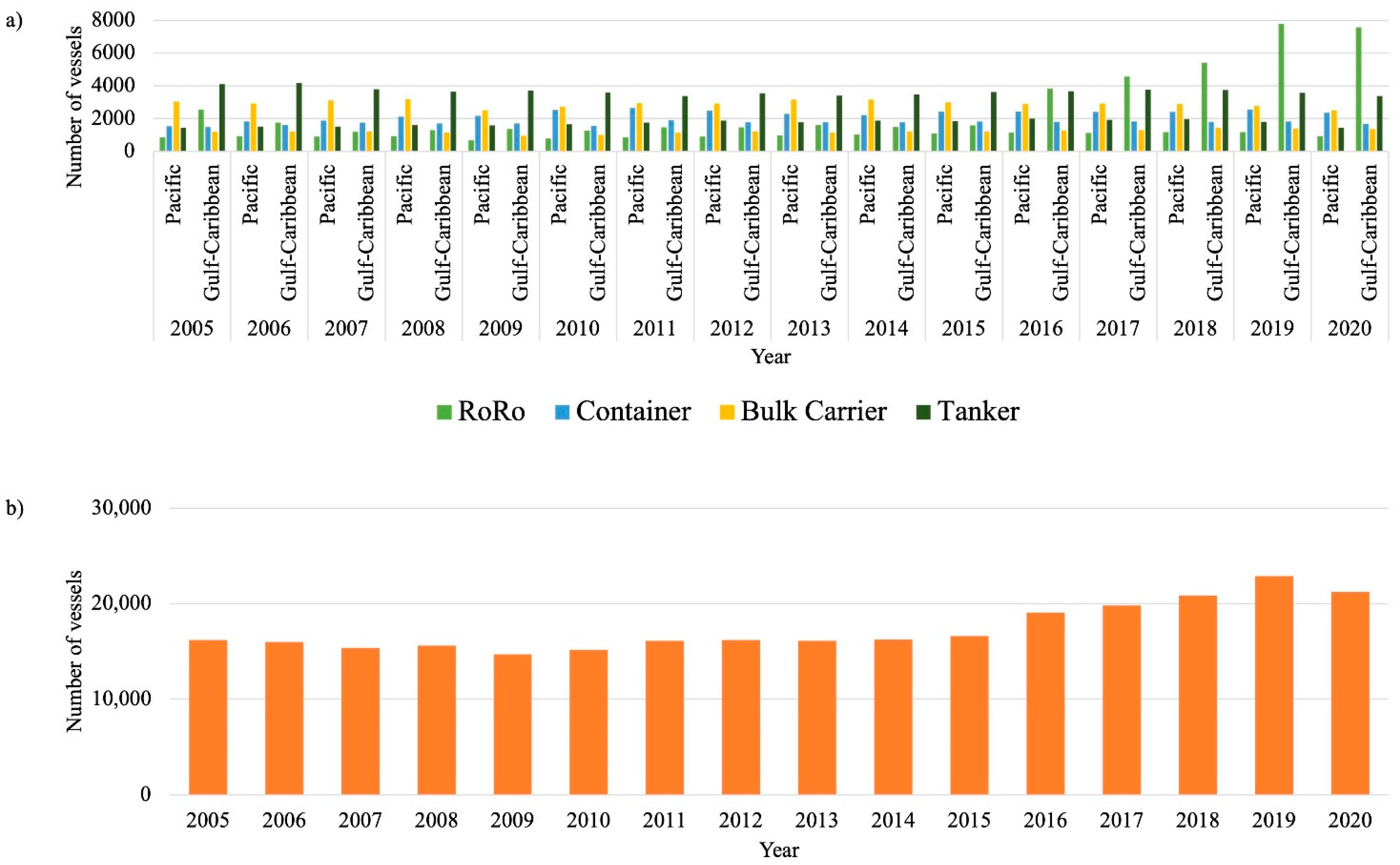
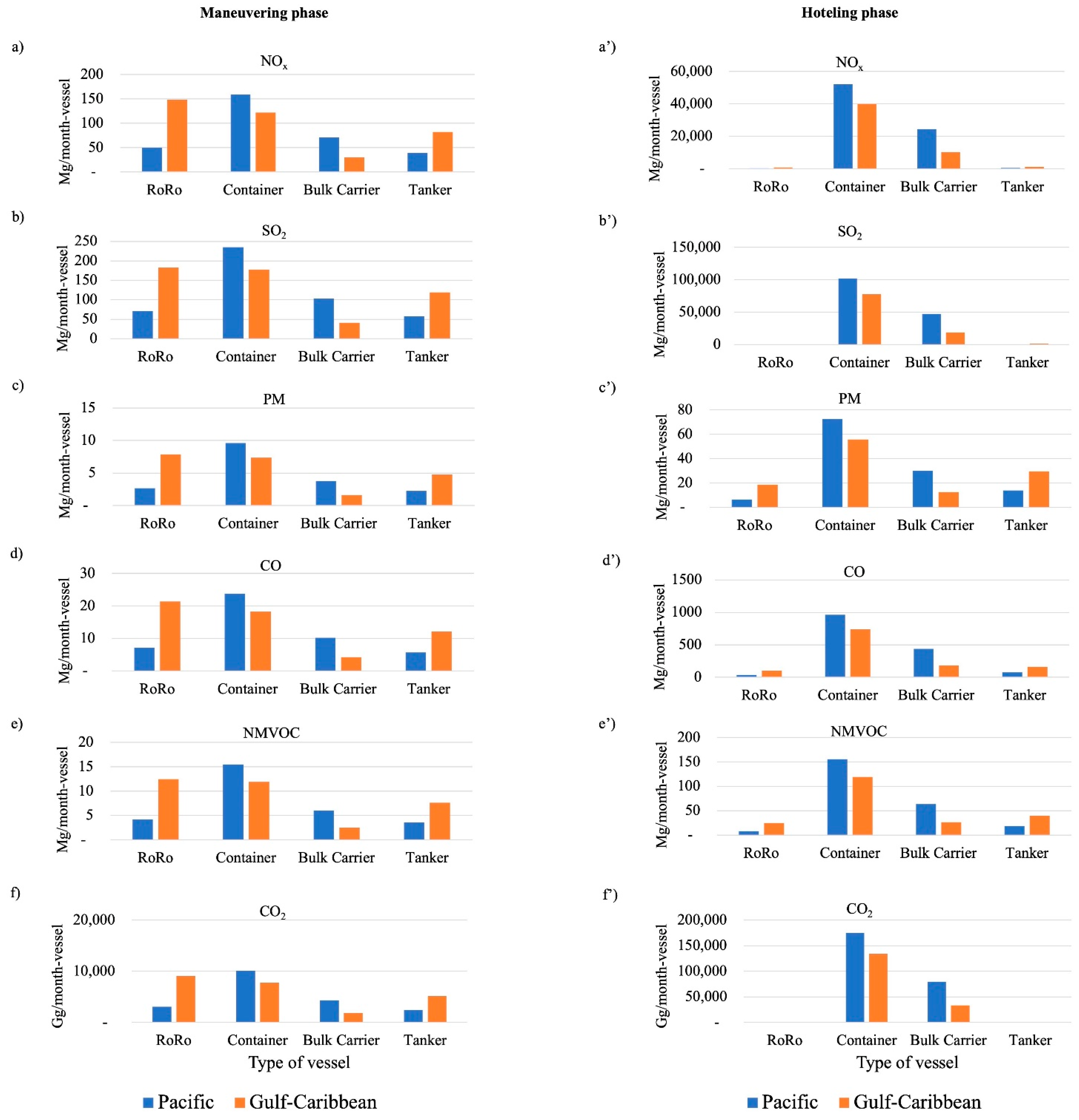
4.1. Arrival of the Vessels

Arrivals by type of vessel at Pacific and Gulf-Caribbean ports from 2005 to 2020 are shown in Figure 3a, with total arrivals shown in Figure 3b. RoRo and Tankers have had a greater boom in the Gulf-Caribbean (Figure 3a), and since 2016 there has been a gradual increase in the RoRo with 7782 ± 566 vessels for 2019, and an average of 3657 ± 58 Tanker vessels annually. The movement of Container and Bulk Carrier is greater in the Pacific, where on average 2269 ± 64 vessels and 2912 ± 44 vessels are registered per year, respectively. The average number of vessels served from 2005 to 2015 was approximately 16,000 ± 506 (Figure 3b). However, from 2016 to 2019 there was a marked increase in the registration of vessels from 19,068 to 22,875 with ± 708. This increase was mainly due to increases in RoRo ship arrivals in the Gulf-Caribbean at the ports of Dos Bocas and Carmen. The global COVID-19 pandemic had a gradual effect on the movement of vessels in Mexico, with a clear decrease in the arrival of vessels in 2020. However, the RoRo ship type remained the principal mode for movement of merchandise from the Gulf-Caribbean.

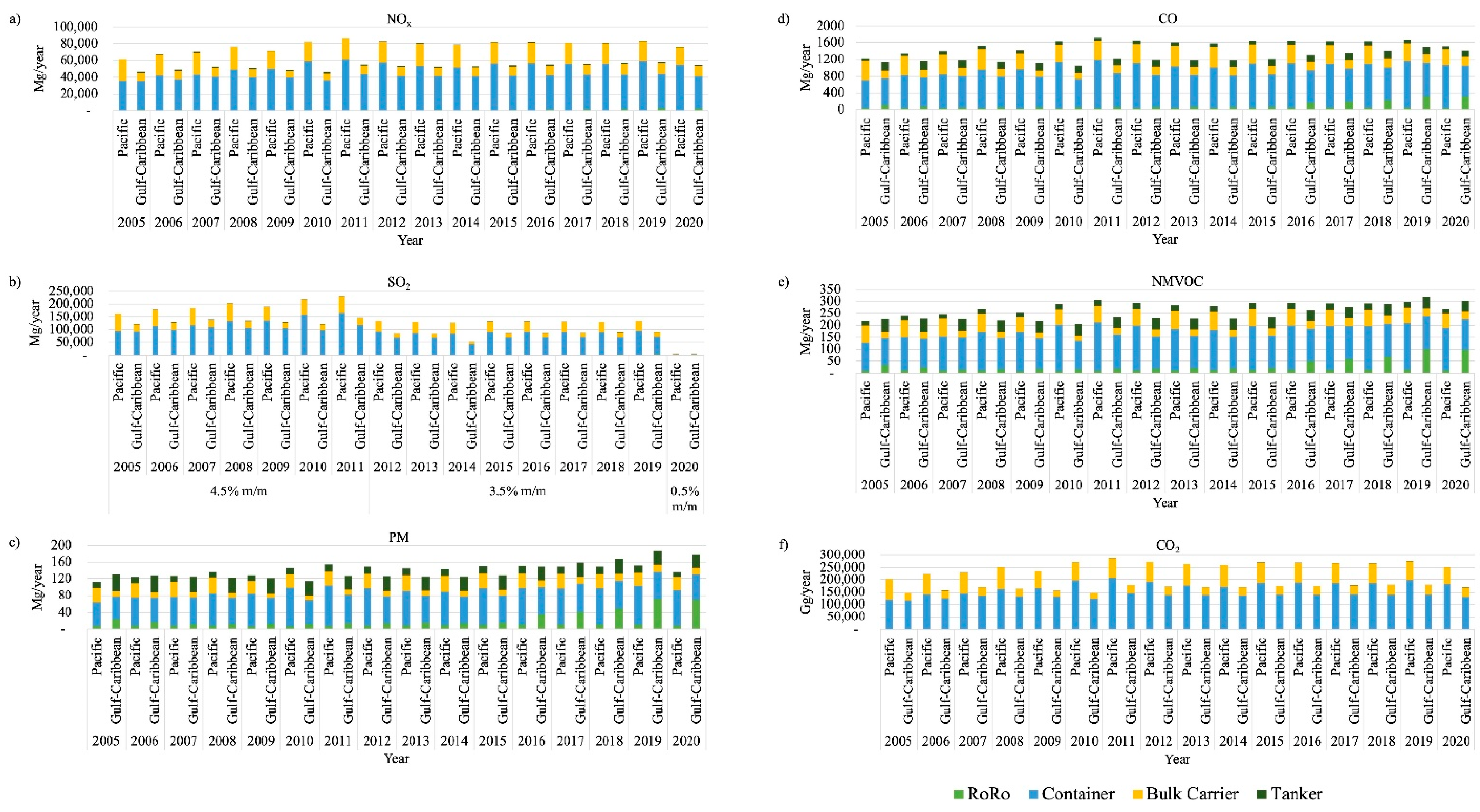
4.2. Atmospheric Emissions from 2005 to 2020 at Pacific and Gulf-Caribbean

Atmospheric emissions by type of vessel in the maneuvering and hoteling phases in Pacific and Gulf-Caribbean ports from 2005 to 2020 are shown in Figure 4 for NOx, SO2, PM, CO, NMVOC and CO2. Atmospheric emission levels in hoteling phase for all vessels at Pacific ports was 77,390 ± 1867 Mg/year for NOx, 150,518 ± 11,727 Mg/year for SO2, 123 ± 3 Mg/year for PM, 1504 ± 37 Mg/year for CO, 247 ± 6 Mg/year for NMVOC and 254,802 ± 6162 Gg/year for CO2. At Gulf-Caribbean ports, the atmospheric emissions were 52,239 ± 920 Mg/year for NOx, 98,748 ± 8004 Mg/year for SO2, 117 ± 5 Mg/year for PM, 1177 ± 33 Mg/year for CO, 211 ± 7 Mg/year for NMVOC and 167,660 ± 2564 Gg/year for CO2 in the hoteling phase. The contribution by type of vessel in hoteling phase atmospheric emissions were 67% Container, 32% Bulk Carrier, 0.8 Tanker, and 0.4% RoRo at Pacific ports, and 76% Container, 20% Bulk Carrier, 2.5% Tanker, and 1.6% RoRo at Gulf-Caribbean ports. The contribution by type of vessel in maneuvering phase atmospheric emissions at Pacific ports were 50% Container, 22% Bulk Carrier, 16% RoRo, and 12% Tanker, and at Gulf-Caribbean ports were 39% RoRo, 32% Container, 21% Tanker, and 8% Bulk Carrier.

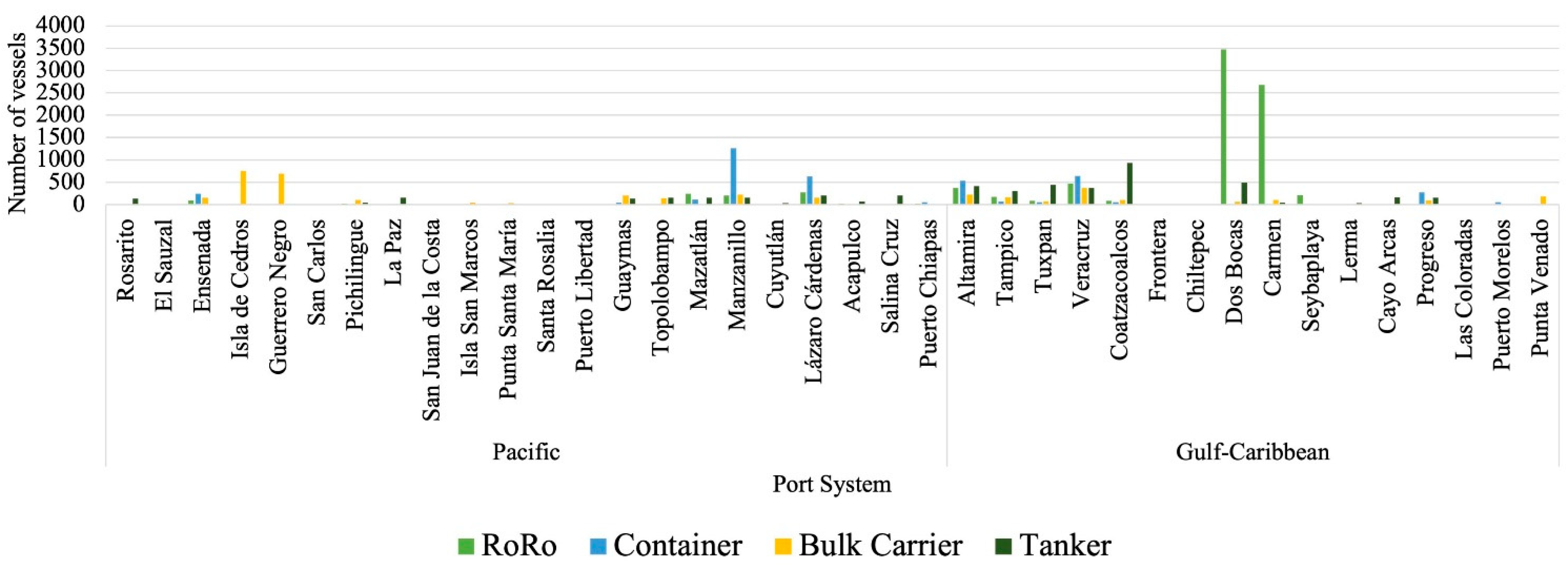
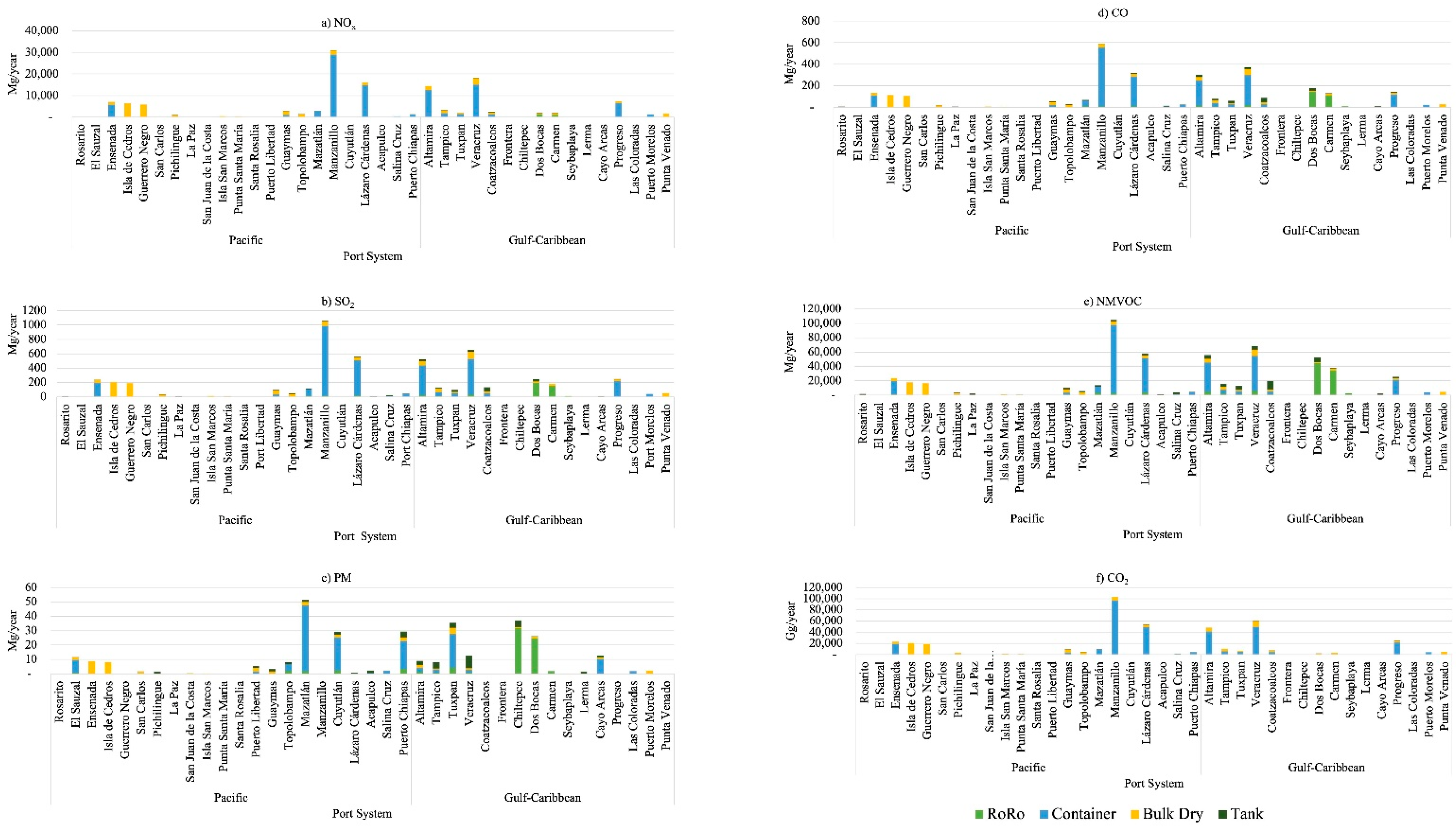
4.3. Distribution of Atmospheric Emissions at Pacific and Gulf-Caribbean Ports

The total emission estimates (Mg/year) by type of vessel from 2005 to 2020, for the maneuvering and hoteling phases, are shown in Figure 5. The atmospheric emission due to the movement of Container and Bulk Carrier was higher at Pacific ports, while RoRo and Tanker emissions were higher at Gulf-Caribbean ports. The atmospheric emissions gradually increased from 2005 to 2011 in the Pacific, with the highest emission occurring in 2011 due to the movement of Container ships. In the Gulf-Caribbean the atmospheric emissions remain approximately constant from 2005 to 2020 due to the movement of Container ships. Emissions from Bulk Carrier and Tanker vessels from 2005 to 2020 have likewise remained approximately constant at both Pacific and Gulf-Caribbean ports. Emissions from RoRo vessels remained steady from 2005 to 2015 for both zones. Starting 2016 the RoRo emissions gradually increased at Gulf-Caribbean ports due to an increasing number of vessels served in that zone, going from 1592 to 7782 with ±483 vessels by 2019 due to the expansion in this zone.
Atmospheric SO2 emissions are reduced when fuel sulfur content decreases. Reductions in sulfur content of 4.5% to 3.5%, 3.5% to 0.5%, and 4.5% to 0.5% were 22%, 86%, and 89%, respectively. In the Pacific, Container and Bulk Carrier constituted the maximum SO2 emissions in the study period, accounting for 67.7% and 31.2%, respectively. Tanker, and RoRo ships contributed 0.7%, and 0.4%, respectively. In the Caribbean Gulf the contributions of Container, Bulk Carrier, Tanker, and RoRo were 76.8%, 18.8%, 2.3%, and 2.2%, respectively. SO2 emissions were significantly reduced in 2020 due to cleaner fuel. For Pacific ports, emissions during 2005–2011, 2012–2019, and 2020 represented 56.6%, 43.3%, and 0.1% of the total during the study period. At Gulf-Caribbean ports the corresponding percentages were 57.9%, 52%, and 0.1%.
We utilized the 2020 database to analyze the atmospheric emission level of each port located in the Pacific and Gulf-Caribbean, as it represents the most current information in Mexico. The number of ships served at each Mexican port are shown in Figure 6. Isla de Cedros, Guerrero Negro, and Punta Venado are characterized by the handling of Bulk Carrier goods, whereas Rosarito, La Paz, Coatzacoalcos, Cayo Arcas, and Progreso are specific to the movement of Fluids or Liquids. Manzanillo, Lázaro Cárdenas, Altamira, and Veracruz. Manzanillo and Lázaro Cárdenas are the principal ports for the movement of Container vessels on the Pacific, and Altamira and Veracruz are the corresponding ports on the Gulf-Caribbean. It should be noted that the number of Container vessel that have been registered in Manzanillo (1256) represents approximately twice those registered at Altamira (535) and Veracruz (642). The movement of general and loose cargo by RoRo vessels has been strengthened in the ports of Dos Bocas and Carmen with 3469 and 2677 vessels, respectively.
The total emissions of (a) NOx, (b) SO2, (c) PM, (d) CO, (e) NMVOC, and (f) CO2 is shown in Figure 7 for each port. The highest emission of atmospheric pollutants comes from Container vessels. The port of Manzanillo has registered the highest atmospheric emission levels, followed by Lázaro Cárdenas, Altamira, and Veracruz. For emissions from Bulk Carrier vessels, the ports of Isla de Cedros and Guerreo Negro represent the highest emissions, followed by the ports of Guaymas, Tampico, and Punta Venado. At the ports of Coatzacoalcos and Dos Bocas the atmospheric emission was dominated by Tanker type vessels, while the RoRo vessels dominated emissions in the ports of Dos Bocas and Carmen. Considering the IMO implementations in 2020 (0.5% sulfur content in marine fuel), the atmospheric emissions of SO2 represented a reduction of 86% to 89% in this year.

5. Conclusions

Maritime traffic in Mexican ports on the Pacific consisted of 2912 ± 44 vessels for Bulk Carrier, 2269 ± 64 for Container, 1724 ± 40 for Tanker and 971 ± 31 RoRo. For Gulf-Caribbean ports the corresponding values were 3657 ± 58 for Tanker, 2890 ± 566 for RoRo, 1739 ± 27 for Container, and 1218 ± 33 for Bulk Carrier. The frequency of vessel types in the Pacific was 37% Bulk Carrier, 29% Container, 22% Tanker, and 12% RoRo. For the Gulf-Caribbean the frequency was 41% Tanker, 25% RoRo, 20% Container, and 13% Bulk Carrier.
The hoteling phase contributions to the total (hoteling + maneuver phases) atmospheric vessels emissions in the Pacific was 60% NOx, 60% CO2, 59% SO2, 56% CO, 54% NMVOC, 51% PM. A difference in atmospheric emission of 18% was found for the Pacific and Gulf-Caribbean in the maneuvering phase, and 39% for the hoteling phase.
Maritime traffic at Pacific ports contributes 60% of total atmospheric emissions and the Gulf-Caribbean 40% during the period of study. The atmospheric emission in the Pacific was 67% Container, 32% Bulk Carrier, 0.8% Tanker, and 0.4% RoRo, while in the Gulf-Caribbean was 76% Container, 19% Bulk Carrier, 3% Tanker, and 2% RoRo.
The highest ship emissions from Pacific and Gulf-Caribbean ports were associated with the movement of Container vessels, representing 67% and 76% of total emissions, respectively. The Mexican Port System is thus principally characterized by atmospheric emissions due to the movement of Container vessels.

6. Recommendations

Include the Automatic Identification System of ships arriving in the Pacific and Gulf of Mexico in the estimation of atmospheric emissions considering the three phases of navigation, following the procedures of this study based on the maneuvering and hoteling positions of ships.
Mexico is in the process of maritime and trade development, particularly in the Gulf of Mexico. To protect air quality and ecosystems, it is thus necessary to implement regulations to prevent and minimize the atmospheric emission due to the movement of ships in port.
It is also necessary to include, in Mexican national inventories, other sources of atmospheric emissions due to maritime activities.

7. Future Work

Evaluate air quality through a photochemical model, integrating atmospheric emissions from ships in port with meteorological data to identify the concentration burden to which the population is exposed due to the movement of ships.
Establish a network or networks of ambient air monitoring stations to monitor compliance with air quality according to the Official Mexican Standards due to port systems. This implementation will include a strict Quality Assurance and Quality Control.

Author Contributions

Conceptualization, J.D.W.K., E.G.H., A.L.A.J. and R.E.A.D.; Data curation, R.S.E.; Formal analysis, J.M.B.R.; Investigation, G.F.G., A.L.A.J. and R.E.A.D.; Methodology, G.F.G., R.S.E. and J.M.B.R.; Resources, E.G.H. and R.E.A.D.; Supervision, R.S.E. and J.M.B.R.; Validation, R.S.E.; Visualization, A.L.A.J.; Writing—review and editing, J.D.W.K. All authors have read and agreed to the published version of the manuscript.

Funding

This research did not receive any specific grant from funding agencies in the public, commercial, or not -for-profit sectors.

Institutional Review Board Statement

Not applicable.

Informed Consent Statement

Not applicable.

Data Availability Statement

Not applicable.

Acknowledgments

The authors of this study are grateful for the participation of the staff of the Sección de Contaminación Ambiental at Instituto de Ciencias de la Atmósfera y Cambio Climático at Universidad Nacional Autónoma de México: Pablo Sánchez Álvarez, Elizabeth Vega Rangel, Eduardo Zamora Vargas, Daimy Ávila Rodríguez, Humberto Bravo Witt, José Téllez Hernández, Roberto Morales Yáñez. Instituto de Geografía de la UNAM: Víctor Magaña Rueda and Gustavo Vázquez Cruz. Participation of the staff of the Administración Portuaria Integral de Veracruz (APIVER): Francisco Liaño C., Socaris de la Luz, and David Augusto de la O N. Agreement between APIVER and UNAM: “Evaluación de la calidad del aire, depósito atmosférico y meteorología para desarrollar el programa para la prevención y minimización del posible deterioro ambiental significativo en el Recinto Portuario de Veracruz y en las zonas de interés”. Finally, we acknowledge Instituto de Ciencias de la Atmósfera y Cambio Climático for supporting the postdoctoral appointment of G.F.G. at Universidad Nacional Autónoma de México.

Conflicts of Interest

The authors declare no conflict of interest.

References

  1. Cofala, J.; Amann, M.; Heyes, C.; Wagner, F.; Klimont, Z.; Posch, M.; Schöpp, W.; Tarasson, L.; Jonson, J.E.; Whall, C.; et al. Analysis of Policy Measures to Reduce Ship Emissions in the Context of the Revision of the National Emissions Ceilings Directive; International Institute for Applied Systems Analysis, Norwegian Meteorological Institute and Entec UK Limited: Newcastle, UK, 2007; pp. 17–21. Available online: https://ec.europa.eu/environment/air/pdf/06107_final.pdf (accessed on 20 January 2020).
  2. UNCTAD. United Nations Conference on Trade and Development. Chapter 1: International Maritime Trade and Port Traffic. In Review of Maritime Transport; United Nations Publications: Geneva, Switzerland, 2019; pp. 1–23. Available online: https://unctad.org/webflyer/review-maritime-transport-2019 (accessed on 15 April 2019)ISBN 978-92-1-112958-8. ISSN 0566-7682.
  3. MARPOL 73/78. Marine Pollution 73/78. International Maritime Organization (OMI). International Convention for the Prevention of Pollution from Ships. Available online: https://www.imo.org/en/About/Conventions/Pages/International-Convention-for-the-Prevention-of-Pollution-from-Ships-(MARPOL).aspx (accessed on 10 August 2020).
  4. IMO. International Maritime Organization. Sulfur 2020 Implementation. IMO Issues Additional Guidance. Available online: http://www.imo.org/en/MediaCentre/PressBriefings/Pages/10-MEPC-74-sulphur-2020.aspx (accessed on 10 August 2020).
  5. IMO. International Maritime Organization. El Límite Mundial del Contenido de Azufre. Available online: https://www.imo.org/en/MediaCentre/HotTopics/Pages/Sulphur-2020.aspx (accessed on 10 August 2020).
  6. ENTEC. European Commission. Directorate General Environment. Service Contract on Ship Emissions: Quantification of Ship Emissions; Final Report; ENTEC UK Limited: Newcastle Upon Tyne, UK, 2002; pp. 3–23. Available online: https://ec.europa.eu/environment/air/pdf/chapter2_ship_emissions.pdf (accessed on 3 May 2020).
  7. ENTEC. European Commission. Directorate General Environment. Service Contract on Ship Emissions Inventory; Final Report; ENTEC UK Limited: Newcastle, UK, 2010; pp. 1–66. Available online: https://uk-air.defra.gov.uk/assets/documents/reports/cat15/1012131459_21897_Final_Report_291110.pdf (accessed on 3 May 2020).
  8. EMEP/EEA. European Monitoring and Evaluation Programme/European Environment Agency; Navigation (Shipping); EMEP/EEA: Copenhagen, Denmark, 2019; pp. 1–40. Available online: https://www.eea.europa.eu/publications/emep-eea-guidebook-2019/part-b-sectoral-guidance-chapters/1-energy/1-a-combustion/1-a-3-d-navigation/view (accessed on 3 May 2020).
  9. SCT. Secretaría de Comunicaciones y Transportes, México. Informe Estadístico de los Puertos. 2020. Available online: http://www.sct.gob.mx/index.php?id=198 (accessed on 27 March 2020).
  10. Fuentes, G.G.; Baldasano, R.J.M.; Sosa, E.R.; Granados, H.E.; Zamora, V.E.; Antonio, D.R.E.; Kahl, W.J.D. Estimation of atmospheric emissions from maritime activity in the Veracruz port, Mexico. J. Air Waste Manag. Assoc. 2021, 71, 934–948. [Google Scholar] [CrossRef] [PubMed]
  11. CCA. Comisión Para la Cooperación Ambiental. Reducción de Emisiones Generadas Por El Movimiento de Bienes en El Transporte Marítimo en América del Norte; Evaluación de los efectos de las emisiones de buques en México: Montreal, QC, Canadá, 2018; pp. 1–42. Available online: http://www3.cec.org/islandora/en/item/11787-reducci-n-de-emisiones-generadas-por-el-movimiento-de-bienes-en-el-transporte-es.pdf (accessed on 20 September 2021).
  12. NFCCC. United Nations Framework Convention on Climate Change. Mexico Submits its Climate Action Plan Ahead of 2015 Paris Agreement. 2015. Available online: https://www4.unfccc.int/sites/submissions/INDC/Published%20Documents/Mexico/1/MEXICO%20INDC%2003.30.2015.pdf (accessed on 20 September 2021).
  13. SEGOB-INECC. Gobierno de México. Instituto Nacional de Ecología y Cambio Climático. Inventario Nacional de Emisiones de Gases y Compuestos de Efecto Invernadero. 2018. Available online: https://www.gob.mx/inecc/acciones-y-programas/inventario-nacional-de-emisiones-de-gases-y-compuestos-de-efecto-invernadero (accessed on 20 September 2021).
  14. IPCC. Intergovernmental Panel on Climate Change. Task Force on National Greenhouse Gas Inventories. Inventory Software. 2006. Available online: https://www.ipcc-nggip.iges.or.jp/software/index.html (accessed on 20 September 2021).
  15. INEGyCEI. Inventario Nacional de Emisiones de Gases y Compuestos de Efecto Invernadero. Datos y Recursos de México. 2018. Available online: https://datos.gob.mx/busca/dataset/inventario-nacional-de-emisiones-de-gases-y-compuestos-de-efecto-invernadero-inegycei (accessed on 20 September 2021).
  16. SEGOB-SEMARNAT. Gobierno de México. Secretaría del Medio Ambiente y Recursos Naturales. Inventario Nacional de Emisiones de Contaminantes Criterio INEM. 2019. Available online: https://www.gob.mx/semarnat/acciones-y-programas/inventario-nacional-de-emisiones-de-contaminantes-criterio-inem (accessed on 20 September 2021).
  17. SCT. Secretaría de Comunicaciones y Transportes, México. Informe Estadístico Mensual. Movimiento de Carga, buques y Pasajeros en los Puertos de México. Enero–diciembre, 2019–2020. 2020. Available online: http://www.sct.gob.mx/fileadmin/CGPMM/U_DGP/estadisticas/2020/Mensuales/12_diciembre_2020.pdf (accessed on 27 March 2020).
  18. Trozzi, C.; Vaccaro, R. Air Pollutant Emissions from Ships: High Tyrrhenian Sea Ports Case Study. In Proceedings of the First International Conference PORTS 98 Maritime Engineering and Ports, Genoa, Italy, 28–30 September 1998; pp. 1–11. Available online: https://www.researchgate.net/publication/236857601_Air_pollutant_emissions_from_ships_high_Tyrrhenian_Sea_ports_case_study (accessed on 3 May 2020).
  19. Trozzi, C.; Vaccaro, R. Methodologies for Estimating Air Pollutants Emissions from Ships: A 2006 Update. In Proceedings of the Environment & Transport 2nd International Scientific Symposium, Reims, France, 12–14 June 2006; pp. 1–8. Available online: https://www.researchgate.net/publication/259470337_Methodologies_for_estimating_air_pollutant_emissions_from_ships_a_2006_update (accessed on 3 May 2020).
  20. Shipping Activities. Emission Inventory Guidebook. In National Sea Traffic, National Fishing, International Sea Traffic, Inland Goods Carrying Vessels; European Environment Agency: Copenhagen, Denmark, 2002. [Google Scholar]
  21. Cooper, D.; Gustafsson, T. Methodology for calculating emissions from ships: 1. Update of emission factors. In Swedish Methodology for Environmental Data; SMED; Swedish Meteorological and Hydrological Institute: Norrkoping, Sweden, 2004; pp. 13–28. Available online: https://www.diva-portal.org/smash/get/diva2:1117198/FULLTEXT01.pdf (accessed on 17 January 2020)ISSN 1652-4179.
  22. USEPA. United States for Environmental Protection Agency. Chapter 2: Ocean Going Vessels. In Current Methodologies in Preparing Mobile Source Port-Related Emission Inventories; Final Report; United States for Environmental Protection Agency: Washington, DC, USA, 2009; pp. 1–26. Available online: https://www.epa.gov/sites/production/files/2016-06/documents/2009-port-inventory-guidance.pdf (accessed on 2 November 2019).
  23. NEAA. Netherlands Environmental Assessment Agency. Methodologies for Estimating Shipping Emissions in the Netherlands. In A Documentation of Currently used Emission Factors and Related Activity Data; NEAA. Netherlands Environmental Assessment Agency: AH Bilthoven, The Netherlands, 2010; pp. 13–38. Available online: https://www.researchgate.net/publication/277223271_Methodologies_for_estimating_shipping_emissions_in_the_Netherlands_A_documentation_of_currently_used_emission_factors_and_data_on_related_activity (accessed on 20 June 2020)ISSN 1875-2314.
  24. Trozzi, C. Emission Estimate Methodology for Maritime Navigation. USEPA. In Proceedings of the 19th International Emissions Inventory Conference, San Antonio, TX, USA, 20–30 September 2010; pp. 1–11. Available online: https://www.researchgate.net/publication/233387511_Emission_estimate_methodology_for_maritime_navigation (accessed on 20 June 2020).
  25. Venturini, G.; Iris, C.; Kontovas, C.A.; Larsen, A. The multi-port berth allocation problem with speed optimization and emission considerations. Transp. Res. Part D Transp. Environ. 2017, 54, 142–159. [Google Scholar] [CrossRef] [Green Version]
  26. Zhang, X.; Lam, J.S.L.; Çağatay, I. Cold chain shipping mode choice with environmental and financial perspectives. Transp. Res. Part D Transp. Environ. 2020, 87, 102537. [Google Scholar] [CrossRef]
  27. Johansson, L.; Jalkanen, J.-P.; Kukkonen, J. Global assessment of shipping emissions in 2015 on a high spatial and temporal resolution. Atmos. Environ. 2017, 167, 403–415. [Google Scholar] [CrossRef]
  28. Jalkanen, J.-P.; Brink, A.; Kalli, J.; Pettersson, H.; Kukkonen, J.; Stipa, T. A modelling system for the exhaust emissions of marine traffic and its application in the Baltic Sea area. Atmos. Chem. Phys. Discuss. 2009, 9, 9209–9223. [Google Scholar] [CrossRef] [Green Version]
  29. Jalkanen, J.-P.; Johansson, L.; Kukkonen, J.; Brink, A.; Kalli, J.; Stipa, T. Extension of an assessment model of ship traffic exhaust emissions for particulate matter and carbon monoxide. Atmos. Chem. Phys. Discuss. 2012, 12, 2641–2659. [Google Scholar] [CrossRef] [Green Version]
  30. Jalkanen, J.-P.; Johansson, L.; Kukkonen, J. A comprehensive inventory of the ship traffic exhaust emissions in the Baltic Sea from 2006 to 2009. Ambio 2014, 43, 311–324. [Google Scholar] [CrossRef] [Green Version]
  31. Simonsen, M.; Walnum, H.J.; Gössling, S. Model for Estimation of Fuel Consumption of Cruise Ships. Energies 2018, 11, 1059. [Google Scholar] [CrossRef] [Green Version]
  32. Toscano, D.; Murena, F. Atmospheric ship emissions in ports: A review. Correlation with data of ship traffic. Atmos. Environ. X 2019, 4, 100050. [Google Scholar] [CrossRef]
  33. Zhang, L.; Meng, Q.; Fwa, T.F. Big AIS data based spatial-temporal analyses of ship traffic in Singapore port waters. Transp. Res. Part E Logist. Transp. Rev. 2019, 129, 287–304. [Google Scholar] [CrossRef]
  34. Browning, L.; Bailey, K. Current Methodologies and Best Practices in Preparing Port Emissions Inventories. Final Report. USEPA. 2006. Available online: https://ntrl.ntis.gov/NTRL/dashboard/searchResults/titleDetail/PB2006112993.xhtml (accessed on 20 November 2019).
  35. Dalsoren, S.B.; Eide, M.S.; Endresen, O.; Mjelde, A.; Gravir, G.; Isaken, I.S.A. Update on emissions and environment impacts from the international fleet of ships: The contribution from major ship types and ports. Atmos. Chem. Phys. 2009, 9, 2171–2194. [Google Scholar] [CrossRef] [Green Version]
  36. Moreno-Gutiérrez, J.; Calderay, F.; Saborido, N.; Boile, M.; Valero, R.R.; Durán-Grados, V. Methodologies for estimating shipping emissions and energy consumption: A comparative analysis of current methods. Energy 2015, 86, 603–616. [Google Scholar] [CrossRef]
  37. Hulskotte, J.; van der Gon, H.D. Fuel consumption and associated emissions from seagoing ships at berth derived from an on-board survey. Atmos. Environ. 2010, 44, 1229–1236. [Google Scholar] [CrossRef]
  38. USEPA. United States for Environmental Protection Agency. Analysis of Commercial Marine Vessels Emissions and Fuel Consumption Data; USEPA: Washington, DC, USA, 2000. [Google Scholar]
  39. Corbett, J.J.; Koehler, H.W. Updated emissions from ocean shipping. J. Geophys. Res. 2003, 108, 4650. [Google Scholar] [CrossRef]
  40. Eyring, V.; Köhler, H.W.; Van Aardenne, J.; Lauer, A. Emissions from international shipping: 1. The last 50 years. J. Geophys. Res. Space Phys. 2005, 110, 17305. [Google Scholar] [CrossRef]
  41. Rodríguez, G.D.M.; Martin-Alcalde, E.; Murcia-González, J.; Saurí, S. Evaluating air emission inventories and indicators from cruise vessels at ports. WMU J. Marit. Aff. 2017, 16, 405–420. [Google Scholar] [CrossRef] [Green Version]
  42. Zhang, Y.; Gu, J.; Wang, W.; Peng, Y.; Wu, X.; Feng, X. Inland port vessel emissions inventory based on Ship Traffic Emission Assessment Model–Automatic Identification System. Adv. Mech. Eng. 2017, 9, 1–9. [Google Scholar] [CrossRef]
  43. Carletti, S.; Latini, G.; Passerini, G. Air pollution and port operations: A case study and strategies to clean up. Sustain. City VII 2012, 1, 391–403. [Google Scholar] [CrossRef]
  44. Gutiérrez, J.; Grados, V.; Uriondo, Z.; Llamas, J. Emission-factor uncertainties in maritime transport in the Strait of Gibraltar, Spain. Atmos. Atmos. Meas. Tech. Discuss. 2012, 5, 5953–5991. [Google Scholar] [CrossRef]
  45. Corbett, J.J.; Winebrake, J.J.; Green, E.H.; Kasibhatla, P.; Eyring, V.; Lauer, A. Mortality from Ship Emissions: A Global Assessment. Environ. Sci. Technol. 2007, 41, 8512–8518. [Google Scholar] [CrossRef]
  46. Smith, T.; Jalkanen, J.; Anderson, B.A.; Corbett, J.J.; Faber, J.; Hanayama, S.; O’Keeffe, E.; Parker, S.; Johansson, L.; Aldous, L.; et al. Third IMO GHG Study; International Maritime Organization: London, UK, 2014; Available online: https://www.researchgate.net/publication/281242722_Third_IMO_GHG_Study_2014_Executive_Summary_and_Final_Report (accessed on 10 December 2019).
  47. Styhre, L.; Winnes, H.; Black, J.; Lee, J.; Le-Griffin, H. Greenhouse gas emissions from ships in ports–Case studies in four continents. Transp. Res. Part D Transp. Environ. 2017, 54, 212–224. [Google Scholar] [CrossRef]
  48. Iris, Ç.; Lam, J.S.L. A review of energy efficiency in ports: Operational strategies, technologies and energy management systems. Renew. Sustain. Energy Rev. 2019, 112, 170–182. [Google Scholar] [CrossRef]
  49. Merk, O. International Transport Forum. Shipping Emissions in Ports; International Transport Forum: Paris, France, 2014; Available online: https://www.itf-oecd.org/sites/default/files/docs/dp201420.pdf (accessed on 24 October 2019).
  50. Knežević, V.; Radonja, R.; Dundović, Č. Emission Inventory of Marine Traffic for the Port of Zadar. Pomorstvo 2018, 32, 239–244. [Google Scholar] [CrossRef] [Green Version]
  51. Cullinane, K.; Tseng, P.-H.; Wilmsmeier, G. Estimation of container ship emissions at berth in Taiwan. Int. J. Sustain. Transp. 2016, 10, 466–474. [Google Scholar] [CrossRef]
  52. Yang, D.-Q.; Kwan, S.H.; Lu, T.; Fu, Q.-Y.; Cheng, J.-M.; Streets, D.G.; Wu, Y.-M.; Li, J.-J. An Emission Inventory of Marine Vessels in Shanghai in 2003. Environ. Sci. Technol. 2007, 41, 5183–5190. [Google Scholar] [CrossRef]
  53. Deniz, C.; Durmuşoğlu, Y. Estimating shipping emissions in the region of the Sea of Marmara, Turkey. Sci. Total. Environ. 2008, 390, 255–261. [Google Scholar] [CrossRef]
  54. Tzannatos, E. Ship emissions and their externalities for the port of Piraeus–Greece. Atmos. Environ. 2010, 44, 400–407. [Google Scholar] [CrossRef]
  55. Gibbs, D.; Rigot-Muller, P.; Mangan, J.; Lalwani, C. The role of sea ports in end-to-end maritime transport chain emissions. Energy Policy 2014, 64, 337–348. [Google Scholar] [CrossRef] [Green Version]
  56. McArthur, D.P.; Osland, L. Ships in a city harbour: An economic valuation of atmospheric emissions. Transp. Res. Part D Transp. Environ. 2013, 21, 47–52. [Google Scholar] [CrossRef]
  57. Cullinane, K.; Cullinane, S. Atmospheric Emissions from Shipping: The Need for Regulation and Approaches to Compliance. Transp. Rev. 2013, 33, 377–401. [Google Scholar] [CrossRef]
  58. Deniz, C.; Kilic, A.; Cıvkaroglu, G. Estimation of shipping emissions in Candarli Gulf, Turkey. Environ. Monit. Assess. 2010, 171, 219–228. [Google Scholar] [CrossRef] [PubMed]
  59. Papaefthimiou, S.; Maragkogianni, A.; Andriosopoulos, K. Evaluation of cruise ships emissions in the Mediterranean basin: The case of Greek ports. Int. J. Sustain. Transp. 2016, 10, 985–994. [Google Scholar] [CrossRef]
  60. Whall, C.; Stavrakaki, A.; Ritchie, A.; Green, C.; Shialis, T.; Minchin, W.; Cohen, A.; Stokes, R. Concawe. Ship Emissions Inventory-Mediterranean Sea; Final Report; Entec UK Limited: Newcastle, UK, 2007; p. 47. [Google Scholar]
  61. PAQS. Port Air Quality Strategies. Department of Transport. Moving Britain Ahead. London. 2002. Available online: https://assets.publishing.service.gov.uk/government/uploads/system/uploads/attachment_data/file/815665/port-air-quality-strategies.pdf (accessed on 20 March 2020).
  62. Wang, X.; Shen, Y.; Lin, Y.; Pan, J.; Zhang, Y.; Louie, P.K.K.; Li, M.; Fu, Q. Atmospheric pollution from ships and its impact on local air quality at a port site in Shanghai. Atmos. Chem. Phys. Discuss. 2019, 19, 6315–6330. [Google Scholar] [CrossRef] [Green Version]
  63. AQMB. Air Quality Monitoring in Barcelona Port, 2020. Available online: http://www.portdebarcelona.cat/en/web/el-port/108 (accessed on 28 August 2020).
  64. AQMLA. Air Quality Monitoring. Port Los Angeles Harbor. 2020. Available online: https://www.portoflosangeles.org/environment/air-quality/air-quality-monitoring (accessed on 28 August 2020).
  65. Saraçoğlu, H.; Deniz, C.; Kılıç, A. An Investigation on the Effects of Ship Sourced Emissions in Izmir Port, Turkey. Sci. World J. 2013, 2013, 218324. [Google Scholar] [CrossRef]
  66. Endresen, Ø.; Sørgård, E.; Sundet, J.K.; Dalsøren, S.B.; Isaksen, I.S.A.; Berglen, T.F.; Gravir, G. Emission from international sea transportation and environmental impact. J. Geophys. Res. Atoms. 2003, 108. [Google Scholar] [CrossRef]
  67. Viana, M.; Hammingh, P.; Colette, A.; Querol, X.; Degraeuwe, B.; De Vlieger, I.; Van Aardenne, J. Impact of maritime transport emissions on coastal air quality in Europe. Atmos. Environ. 2014, 90, 96–105. [Google Scholar] [CrossRef]
  68. Lloyd’s Register. Sulphur 2020: What’s Your Plan? In Guidance for Shipowners and Operators on MARPOL Annex VI Sulphur Regulation; Lloyd’s Register Group Limited: London, UK, 2018; Available online: https://www.lr.org/en/sulphur-2020/ (accessed on 25 September 2020).
  69. ENTEC; European Commission; Directorate General Environment. Ship Emissions Inventory–Mediterranean Sea; Final Report, A report for CONCAWE; ENTEC UK Limited: Newcastle Upon Tyne, UK; European Commission: Brussels, Belgium; Directorate General Environment: Brussels, Belgium, 2007. [Google Scholar]
  70. Nicewicz, G.; Tarnapowicz, D. Assessment of Marine Auxiliary Engines Load Factor in Ports. Manag. Syst. Prod. Eng. 2012, 3, 12–17. Available online: https://www.researchgate.net/publication/298026922_Assessment_of_marine_auxiliary_engines_load_factor_in_ports (accessed on 15 October 2019).
  71. ENTEC. European Commission. Directorate General Environment. Service Contract on Ship Emissions: Assignment Abatement and Market-Based Instruments. Task 1 Preliminary Assignment of Ship Emissions to European Countries, 2005. Available online: https://ec.europa.eu/environment/air/pdf/task1_asign_report.pdf (accessed on 22 May 2020).
Figure 1. Location of the Mexican ports. Own elaboration considering to data available from [9].
Jmse 09 01186 g001
Figure 2. Information required to estimate atmospheric emissions in Mexico.
Jmse 09 01186 g002
Figure 3. Arrivals by (a) type of vessel and (b) total vessels from 2005 to 2020.
Jmse 09 01186 g003
Figure 4. Atmospheric emissions by type of vessel in maneuver for (a) NOx, (b) SO2, (c) PM, (d) CO, (e) NMVOC and (f) CO2, and hoteling for (a’) NOx, (b’) SO2, (c’) PM, (d’) CO, (e’) NMVOC and (f’) CO2.
Jmse 09 01186 g004
Figure 5. Atmospheric emissions from 2005 to 2020 for (a) NOx, (b) SO2, (c) PM, (d) CO, (e) NMVOC and (f) CO2.
Jmse 09 01186 g005
Figure 6. Arrivals by type of vessel at each Mexican port during 2020.
Jmse 09 01186 g006
Figure 7. Atmospheric emission for (a) NOx, (b) SO2, (c) PM, (d) CO, (e) NMVOC, and (f) CO2 for each port and type of vessel.
Jmse 09 01186 g007
Table 1. Arrival of vessels in each port on the Pacific and Gulf-Caribbean during 2020.
Port NameStateRoRoContainerBulk CarrierTankerTotal
PacificRosaritoBC---133133
El SauzalBC-----
EnsenadaBC932431534493
Isla de CedrosBC-0750-750
Guerrero NegroBCS-0688-688
San CarlosBCS-001111
PichilingueBCS24010240166
La PazBCS1000150160
San Juan de la CostaBCS--6-6
Isla San MarcosBCS--47-47
Punta Santa MaríaBCS--30-30
Santa RosaliaBCS--0--
Puerto LibertadSON--0--
GuaymasSON1941203137400
TopolobampoSIN10-148154312
MazatlánSIN2471160151514
ManzanilloCOL20312562201501829
CuyutlánCOL---3636
Lázaro CárdenasMICH2706331572011261
AcapulcoGRO28--74102
Salina CruzOAX1133203220
Puerto ChiapasCHIS24549-87
TOTAL9292356251614447245
Gulf-CaribbeanAltamiraTMPS3725352214181546
TampicoTMPS17872167307724
TuxpanVER845970439652
VeracruzVER4746423713741861
CoatzacoalcosVER87531079341181
FronteraTAB-----
ChiltepecTAB-----
Dos BocasTAB3469-604904019
CarmenCAMP2677-101412819
SeybaplayaCAMP210---210
LermaCAMP---3737
Cayo ArcasCAMP---167167
ProgresoYUC1627796158547
Las ColoradasYUC-----
Puerto MorelosQ.ROO-52--52
Punta VenadoQ.ROO--184-184
TOTAL756716901377336513,999
BC: Baja California, BCS: Baja California Sur, SON: Sonora, SIN: Sinaloa, COL: Colima, MICH: Michoacán, GRO: Guerrero, OAX: Oaxaca, CHIS: Chiapas, TMPS: Tamaulipas, VER: Veracruz, TAB: Tabasco, CAMP: Campeche, YUC; Yucatán y Q.ROO: Quintana-Roo.
Table 2. Technical data for each type of vessel considered in this study. Data available for Sample of Ships, Total GT, and Power Installed of ME were adapted from [7,69].
Ship TypeSample of Ships, [7,69]Total GT
[7,69]
Average GTPower Installed of the ME, [69]Power of the ME, kWRatio AE/MEPower of the AE, kW
RoRo10,670182,580,94417,112 164.578 G T 0.4350 11,4250.394456
Container13,318324,977,36124,401 2.9165 G T 0.8719 19,5090.254877
Bulk Carrier711198,055,08913,789 35.912 G T 0.5276 54860.382085
Tanker11,489213,358,95018,571 14.755 G T 0.6082 58240.291689
Table 3. Emission factors (gpollutant/kW-h) for estimating atmospheric emissions in Mexico. Data available for Emission Factors were adapted from [7,8,22].
PositionEngineEmission Factors [7,8,22]
NOxSO2COPMNMVOCCO2
4.5% a3.5% b0.5% c
Maneuver
gpollutant/kW-h
ME9.920.0715.612.231.70.91.5710
AE1319.5315.192.171.60.30.4690
Hoteling
gpollutant/kW-h
AE1319.5315.192.171.60.30.4690
a Sulphur content in Marine Fuel Oil. IMO Regulation Period: Before 2000 to 31 December 2011. b Sulphur content in Marine Fuel Oil. IMO Regulation Period: 1 January 2012 to 31 December 2019. c Sulphur content in Marine Fuel Oil. IMO Regulation Period: 1 January 2020 to currently.
Table 4. Maneuvering and hoteling time (h) for each ship type. Data adapted from [6,71].
Type of VesselSpent Time
Maneuver., h
Spent Time
Hoteling, h
References
RoRo1.025[6,71]
Container1.026
Bulk Carrier1.064
Tanker1.042
Publisher’s Note: MDPI stays neutral with regard to jurisdictional claims in published maps and institutional affiliations.

