1. Introduction
The ability to accurately estimate the salinity intrusion and mixing in estuaries is critical to coastal engineering and our understanding of estuarine dynamics. Saltwater intrusion is regulated primarily by the tide and river runoff [
1] and influenced by factors including topography, wind stress, vertical mixing, tidal range, and freshwater flow [
2,
3,
4].
However, the real-time monitoring of river discharge is necessary to analyze the estuary functioning at an adequate level of precision and to obtain accurate measurements of temporal variations in the freshwater inflow regime over spans of time ranging from several minutes to multiple years [
5].
Continuous and long-term readings of freshwater inputs to estuaries are acquired using stage–discharge rating curves established empirically at upstream gauging stations [
6,
7]. In estuaries influenced by salinity intrusion, estimating the cross-sectional average velocity and discharge from spatial estimation (using limited velocity measurements) is problematic due to the possible distortions in conventional, i.e., log or power law, profiles [
5].
Most methods of estimating the horizontal distribution of salinity and velocity may be classified as either direct or indirect. For direct methods, information about salinity and velocity is typically collected during field observations using various instruments deployed at several locations within the target site at different time periods [
8,
9,
10]. For indirect methods, 1D, 2D, or 3D models are used to simulate the interactions among factors such as river discharge, tidal variation, bathymetry, and wind effect that significantly influence salinity intrusion and mixing mechanisms [
4,
11]. Another indirect method that can monitor 2D salinity distribution in the ocean or along the coastal line is satellite remote sensing technique. This technique has been successfully used to observe sea surface salinity [
12] or to map the structure of river plumes and salinities [
13].
However, the current methods of estimating the horizontal distribution of salinity and velocity in estuaries are impacted by four limiting factors. First, there are uncertainties associated with freshwater supplementation from sources such as tributaries, localized rainfall, and human activities. Moreover, freshwater loss due to diversion and other causes may significantly reduce the accuracy of discharge and salinity measurement estimates which are not typically addressed in related work. Second, the representation of the spatiotemporal evolution of salinity fields in an estuary is inadequate because time and space samples are not included in the instrument data. Using spatial interpolation to obtain the spatial distribution of salinity and temperature generally results in a low quality of estimation. Third, for numerical and analytical models, insufficient observational data limits the interpretation of sensitivity tests. Thus, a significant challenge is how to apply theory appropriately to fill the gaps between the model and observations. Fourth, the large number of instruments that must be deployed over a study site to obtain sufficiently accurate field data, and analyze results add significantly to the overall cost of the system. For example, Vaz et al. [
11] used ten instruments to collect the water temperature and salinity from an 11 km study site. Thus, a cost-effective measurement method able to provide accurate and beneficial information on estuarine physics is needed.
The fluvial acoustic tomography (FAT) system, developed at Hiroshima University in 2008, is a highly versatile hydroacoustic system for investigating hydrological and hydraulic processes. In prior research, the FAT system was used to estimate continuous long-term river flow and streamflow direction [
14,
15], to map the horizontal velocity of the current field in a depthless river [
16], and to measure minimal flow rates in extremely shallow streams [
17]. Based on the above, FAT is a valid system for measuring river discharge and exploring various advanced applications in the water resources domain.
However, most published studies on salinity intrusion, stratification, estuarine circulation, and salinity flux that employed FAT were implemented using a traditional scheme that included an oblique transmission line and several FAT units (e.g., [
18,
19,
20]). Thus, the main objective of this study was to apply the new FAT deployment pattern to investigate the longitudinal distribution of salinity and tidal flow in a tidal channel. This research is expected to answer two important questions: (1) Can alternative FAT system deployment schemes improve flow direction measurement capabilities and cover a wider study area at a relatively lower cost? (2) What is the accuracy of the proposed FAT deployment pattern and what are the associated challenges/difficulties?
The aim of this study was to examine the performance of the proposed scheme using the FAT system in terms of providing sufficiently accurate estimates of river discharge in tidal estuaries using a mesoscale estuary, the Ōta River floodway, in Hiroshima, Japan as a case study. The main novelty of this work is the use of a new scheme for the tomographic deployment of the FAT system. Two pairs of four FAT units were installed along a 700 m length of estuarine floodway in a zigzag configuration. The significance of this work is its exploration of the results of examining the stream velocity on both river banks in both landward and seaward directions.
A short description of the observation area is given in the next section. The methodology used is presented in
Section 3, the results and discussion are presented in
Section 4, and the main conclusions are presented in
Section 5.
2. Observation Site
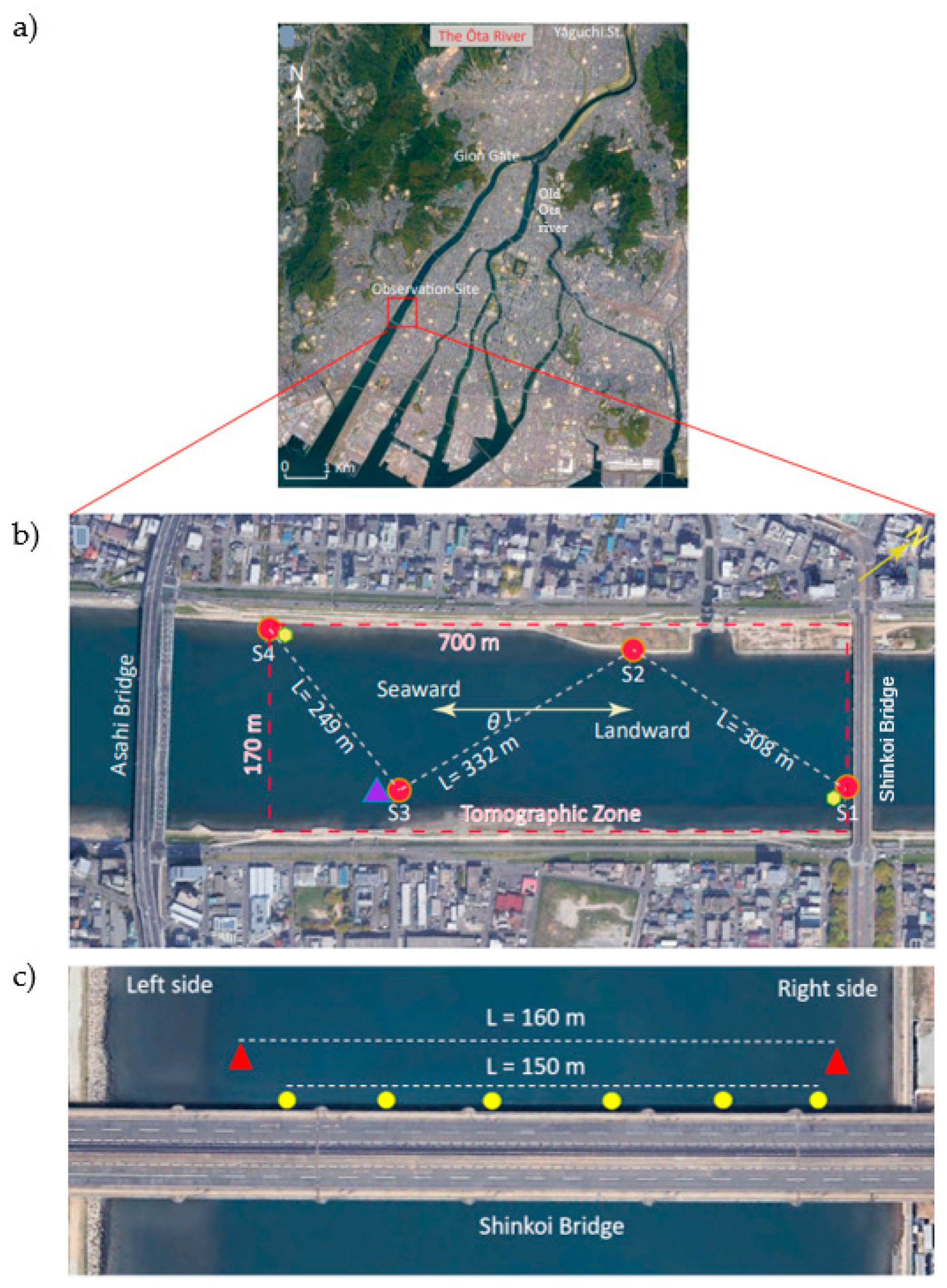
The Ōta River estuary in Hiroshima City, western Japan, was the monitoring site used in this study. A field observation was carried out at the diversion channel, which is a shallow, tidally dominated channel with floodgates located around 9 km upstream from the estuary mouth that restricts the flow of freshwater runoff from further upstream. The estuary has irregular bathymetry with extensive tidal flats and significant variations in the cross-section profiles. The mixed tides in this estuary include diurnal and primary semidiurnal components, and the tidal range at the river mouth ranges from 1.2 m at the neap tide to about 4 m at the extreme spring tide. The Ōta River has vital environmental characteristics, with the downstream section serving as an ecosystem for many tidal species, a large portion of which are oysters.
A map of the study location is shown in
Figure 1. The FAT system was deployed about 4.3 km upstream from the estuary. The tomographic scheme is presented in
Figure 1b, and the Compact CTD and FAT campaigns for validation during a typical spring tide are shown in
Figure 1c. In this study, a series of four FAT units with different transmission lengths were deployed in a zigzag distribution pattern. Assessing the potential advantages of using a zigzag pattern rather than a conventional pattern (i.e., measurement at one cross-section) to trace the velocity behavior over the main channel during flood and ebb tides (i.e., landward and seaward flow directions) was the main focus of this exploration. As shown in
Figure 1b, the tomographic zone is extended over 700 m
170 m.
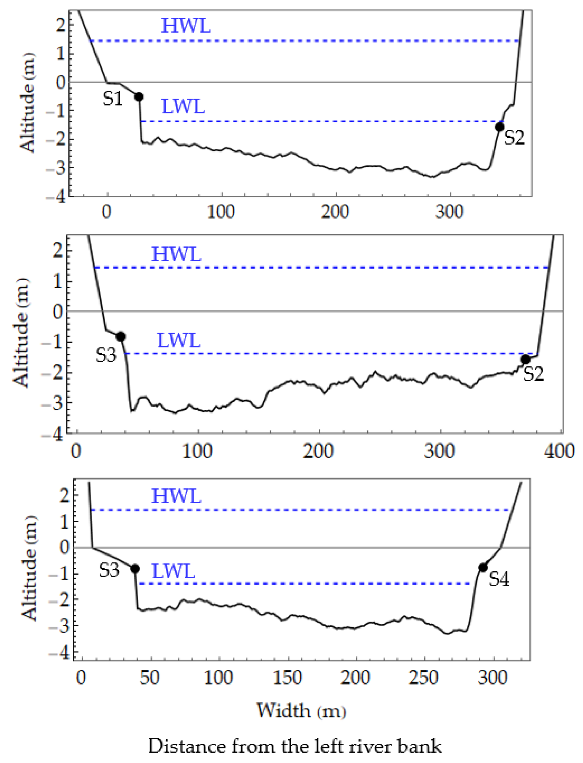
The oblique cross-sections between each pair of acoustic stations are presented in
Figure 2. In general, the riverbed was irregularly shaped and not flat. The freshwater runoff was controlled by the Gion sluice gates (
Figure 1) located 4.5 km upstream from the observation site. During the observation period, the Gion sluice gates were operated under normal conditions, with only one of the three gates partially open and a cross-sectional stream area of 32 m
0.3 m for the spilling flow [
20].
3. Methods and Data Description
3.1. The Fluvial Acoustic Tomography (FAT): Measurement Approach and Data Collection
The FAT is an advanced hydroacoustic instrument designed by Hiroshima University that uses submerged acoustics to observe various hydrological properties of rivers at levels ranging from −0.3 m to −10 m in depth [
16,
17]. FAT emits omnidirectional acoustic signals at different frequencies (mainly between 17–55 kHz). The FAT system contains GPS receivers that help synchronize both FAT units to guarantee the high-precision transmission of pulses. The periodicity of acoustic pulses was 30 secs, synchronized with a GPS clock.
FAT uses the time-of-travel tomography method. The velocity along the transmission line (
u) and speed of sound (
c) are evaluated based on respective travel times, (
tup) and (
tdown), at the upstream and downstream stations, as follows:
where
L is the horizontal spacing between the upstream and downstream stations. For a given cross-section, the section-averaged velocity (
V) and discharge acquired by FAT (
Q) are calculated using the following equations:
where
A (
H) is the cross-sectional area along the ray path as a function of the water depth (
H), and
θ is the angle between the ray path and streamline.
In this work, four broadband transducers with a central frequency of 30 kHz were used to measure the cross-sectional averaged velocity, discharge, and salinity over the period from 28 December 2018 to 16 January 2019, and were deployed as shown in
Figure 1. The horizontal distances are shown in
Figure 1b, with the longest transmission line between S2–S3 (332 m) and the shortest between S3–S4 (249 m).
3.2. Longitudinal Distribution of Salinity, Salinity Gradient, and Dispersion Coefficient
As described by Herman Medwin [
21], the speed of sound in water is generally a function of salinity, water temperature, and depth:
where
T is water temperature (°C),
c is speed of sound (m/s), and
D is depth (m). The valid parameter ranges in Equation (5) are as follows: 0 ≤
T ≤ 35 °C, 0 ≤
D ≤ 1000 m, and 0 ≤
S ≤ 45. This relationship helps estimate the cross-sectional averaged salinity using the speed of sound in water computed by the FAT system.
The salinity gradient and dispersion coefficient may be estimated using the distribution of longitudinal salinity. The longitudinal dispersion coefficient indicates the capacity of a river flow to scatter substances in the longitudinal direction. In a normal channel, the rate of dispersive transport is proportional to the water velocity and longitudinal concentration gradient, which may be calculated using the following equation:
where
S is the section-averaged salinity,
u is the water velocity,
x is the distance upstream from the estuary’s mouth, and
Dx is the longitudinal dispersion coefficient.
3.3. Determination of Flow Direction
The accurate calculation of the flow direction angle is critical to obtaining precise results. Bahreinimotlagh et al. [
15] proposed an equation for calculating the flow direction, which minimizes the potential error factor using four transducers to create two crossed acoustic transmission lines. This equation is based on the continuity condition, and the water discharge of the two related parts should be equal.
Many factors influence the degree of fluctuation in discharge along the channel. However, it was assumed in this study that the short distance of the study site (700 m) made the flow variations negligible. Thus, for simplicity, the degree of fluctuation was not considered in the calculations. Equation (7) was used to calculate the temporal variations in the flow direction obtained from the FAT system data:
where
∅ is the angle between two transmission lines (e.g., S1S2 and S2S3). The
∅ may be expressed as:
where
X1,
X2,
Y1 and
Y2 are determined using the coordinates of the acoustic stations.
A formulation of the structure of the relative error was also proposed in this study that included the following five terms:
The error term
represents the uncertainty in the angle between two crossed paths and has a large impact on the error analysis. The second and third error terms
are errors in the water level measurements. The fourth and last terms
are errors in the mean velocity along the transmission lines. The detailed equations of these error components are shown in
Appendix A.
An important issue to be addressed in discharge computation is how to quantify the error structures in the discharge measurements made by the FAT system. In fact, the discharge estimate of the FAT system is induced by the following terms: (i) errors in water depth measurements, (ii) riverbed uncertainties, (iii) velocity measurements, and (iv) flow direction estimates. The error structures induced by the discharge measurements of the FAT systems [
6] are summarized in Equation (10) below:
Finally, the results of the error calculation process were compared with the results of the moving boat Stream–Pro ADCP (Acoustic Doppler Current Profiler), which measured at the same three transmission lines for 2 days (12–14 December 2019).
3.4. Measurement of Temperature, Depth, and Bathymetry
As mentioned in the previous section, Stream–Pro ADCP (Teledyne RDI Stream–Pro Acoustic Doppler Current Profiler) was used to obtain the data on the bathymetry of the riverbed of the monitored cross-sections and to determine the flow directions for the measured flow. In addition, the discharge data generated by the Stream–Pro ADCP was compared to the discharge estimated by FAT. During the observation period, the moving-boat ADCP was regularly used.
The temporal variations in water temperature were measured using three CT (conductivity and temperature) sensors attached to tripods side-by-side to the S1 station at 0.52 m, S3 station at 0.5 m and S4 station at 0.4 m above the bottom, with the data used to calculate salinity using Equation (5) (see
Figure 1).
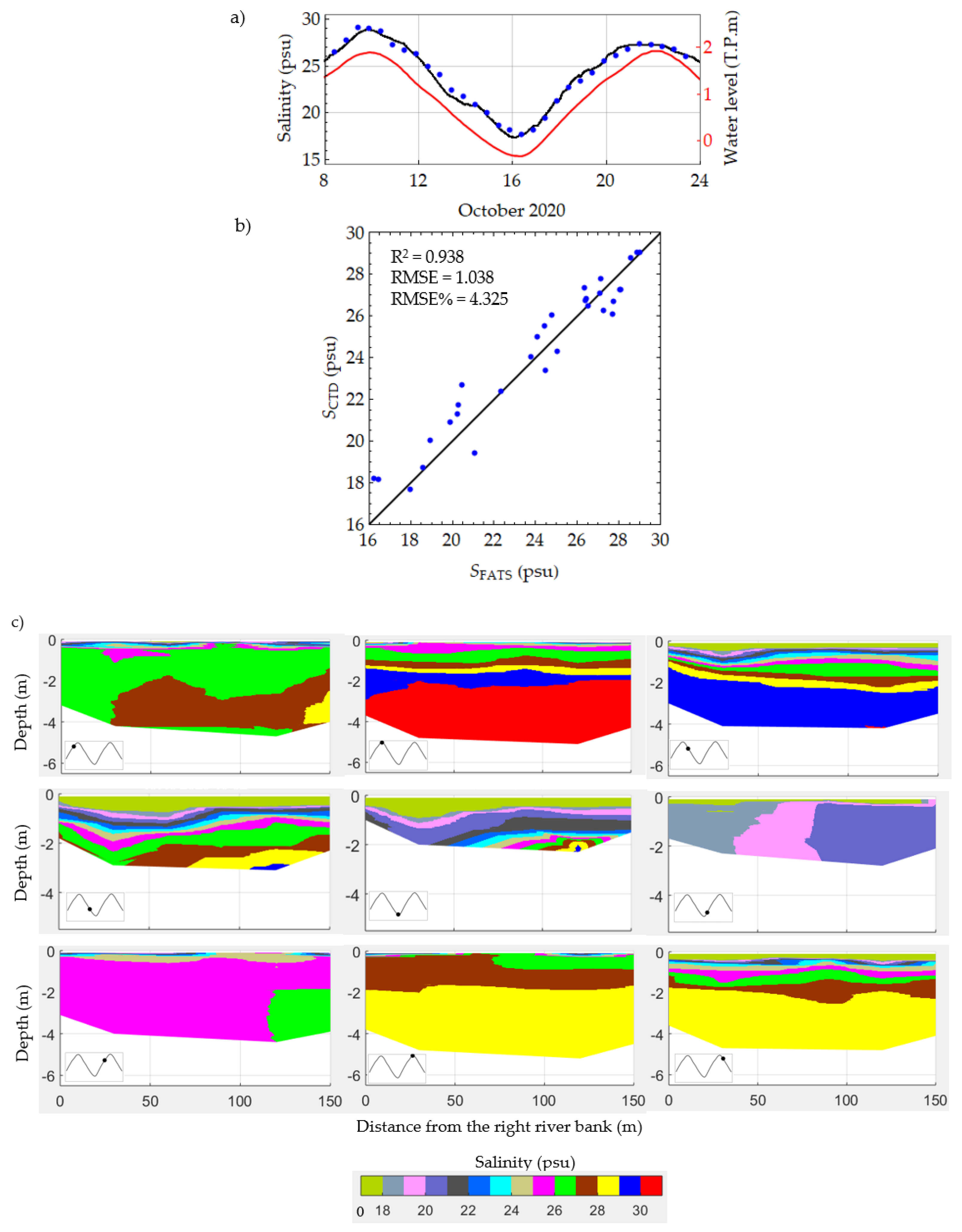
CTD campaigns were carried out at two FAT units concurrently along Shinkoi Bridge during a typical spring tide to confirm the feasibility of using the FAT system to measure the section-average salinity. The measurements of salinity distribution in the cross-section were taken on 2 October 2020, from 08:20 to 23:30 (see
Figure 1c). During these campaigns, two FAT units were deployed on the left and right sides of the river near Shinkoi Bridge with a transmission length of 160 m. The CTD collected the vertical salinity distribution at six points along the bridge every thirty minutes.
The temporal variations in water level (H) were recorded using water loggers, deployed side-by-side at each acoustic station (i.e., at S1, S2, S3, and S4). The water level records provided temporal data on water heights, which were used to measure the temporal variations of the cross-sectional area at each transmission path.
4. Results and Discussion
This work was designed to assess the performance of a promising tomographic system capable of monitoring the cross-sectional average velocity, discharge and salinity variations with high temporal resolutions over long time periods. The observation program in this study ran for three weeks. During the observation, data were occasionally lost because of factors including transducer cable corruption (due to human error, marine transport, etc.) and battery shutdown. However, the obtained data were adequate to describe the tidal dynamics at the target site.
4.1. Temporal Variations in Water Level and Tidal Current Velocity Distribution along the Channel
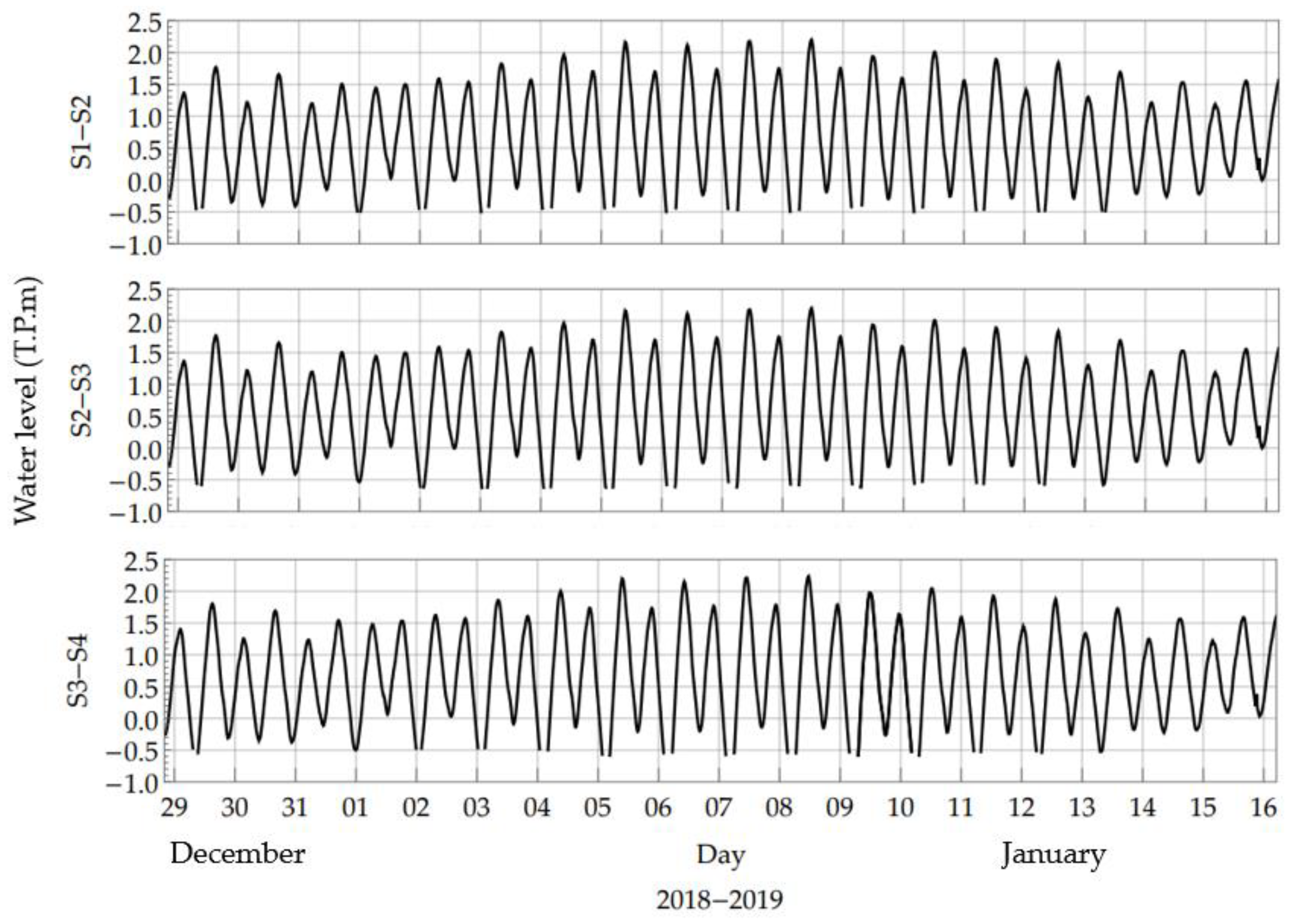
The temporal variations in the water levels recorded at S1–S2, S2–S3, and S3–S4 are shown in
Figure 3. Compared to the average water level in Tokyo Bay (T.P), the water level was integrated to evaluate the temporal variations of the cross-sectional area for each section.
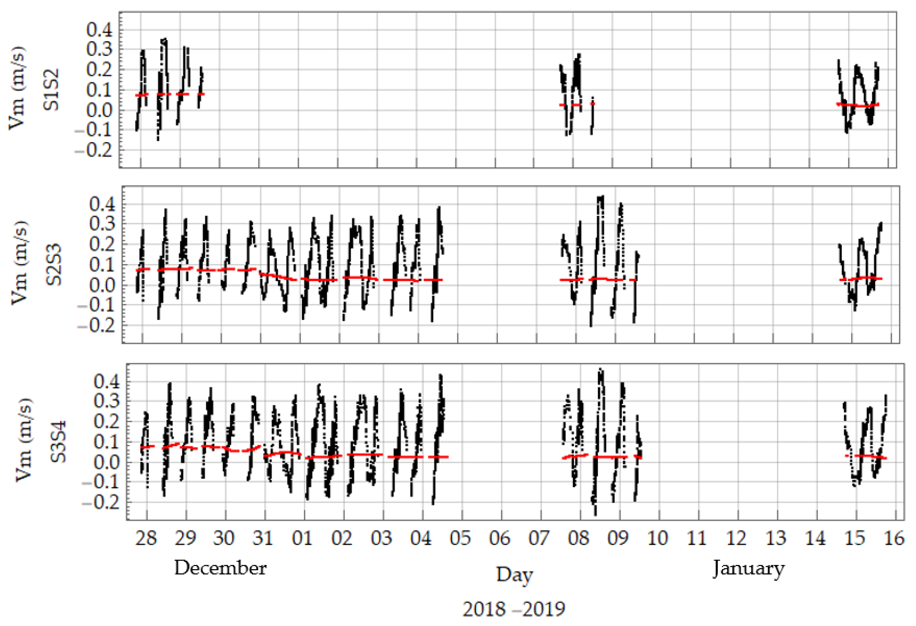
The plotted time series of the tidal current (black) and residual current (red) velocities recorded by the FAT stations are shown in
Figure 4. The missing periods resulted from the abovementioned problems during the monitoring program and the drying out of the transducers. The maximum ebb-tide velocity was roughly 0.45 m/s and the highest value of flood-tide velocity was estimated as −0.2 m/s. The asymmetrical character of the tide indicates that the Ōta River estuary is ebb-dominant.
The S3S4 transmission line registered the highest ebb-tide velocity (approximately −0.75 m/s) on 12 January 2019, and the S1S2 transmission line registered the lowest velocity (approximately −0.3 m/s) on 8 January 2019. An increase in peak ebb-tide velocities was observed in the downstream direction, likely because of the conservation of mass. Moreover, in the S2S3 section (
Figure 4), the velocity fluctuations during neap tides (1–4 January 2019) were smaller than those during spring tides (4–7 January 2019), revealing a significant correlation with water level fluctuation.
The interaction may generate this ebb dominance phenomenon in the Ōta River estuary during the tide between the shallow water area and the varying friction distribution due to the irregular topography (
Figure 2). Previous studies [
22,
23] reported similar findings and claimed that this effect implies that the water surface within the estuary adapts to the tide at the mouth at low water more quickly than at high water. Therefore, the elevation lag between the estuary and ocean is less at low tide than at high tide. This phenomenon results in a steeper tidal curve throughout the ebb tide within the estuary and creates a faster-flowing ebb current.
4.2. Flow Direction Variations
Equation (7) was used to calculate the temporal fluctuations in flow direction using data obtained from the FAT system. The fluctuated ranges of the angle between the flow and transmission lines for all three sections were approximately 2.2 degrees. Moreover, the variations in the mean flow direction over the three cross-sections ranged from 17.3–19.4°, 45.4–47.6°, and from 35.9–38.2°, respectively. Furthermore, the error analysis results of the angle estimation were calculated, with the maximum relative errors shown to be approximately ±6%, which was acceptable.
The estimation of the averaged angles gained from ADCP for the monitored cross-sections were = 18.29° for S1–S2, = 46.33° for S2–S3, and = 37.31° for S3–S4. The minor deviations between the FAT and ADCP estimates further confirmed the acceptable efficiency of obtaining flow direction measurements using FAT.
4.3. Estimating Water Discharge along the Channel
The angles with tidal current velocities and cross-section areas were used to calculate flow rate using Equation (4), as shown in
Figure 5. The variation in water discharge corresponded with that of the tidal current, with the peak discharge during the ebb tides rising to approximately 200 m
3/s. It is evident that the ebb-tide discharges were twice as high as the flood-tide discharges over the study period.
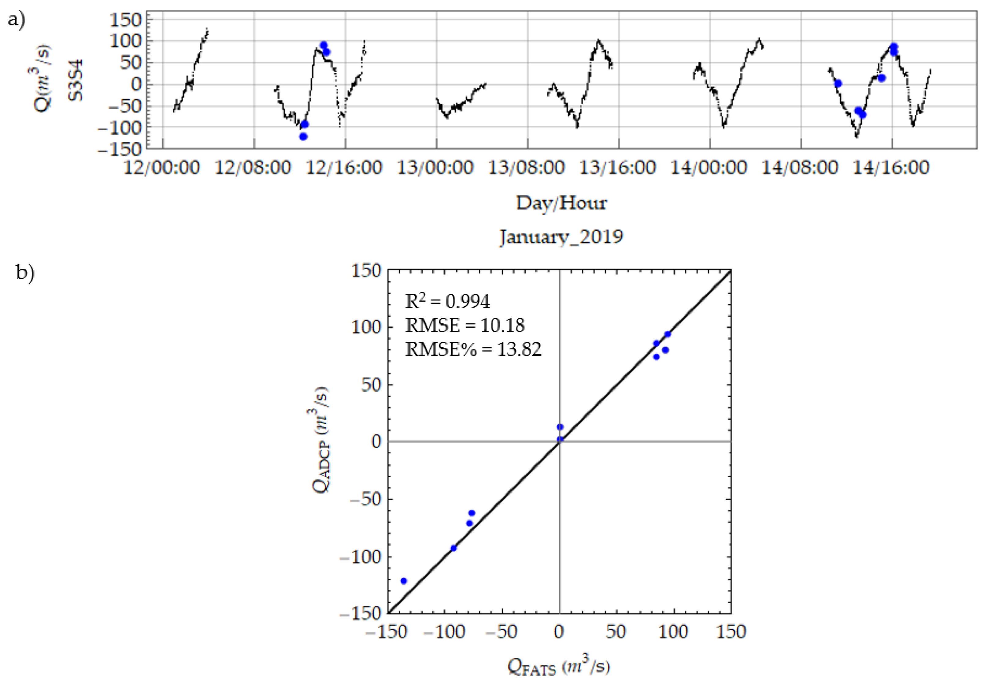
To investigate the quality of the obtained data, the discharge acquired using the FAT system in this study were compared to independent ADCP data acquired from scans of the Asahi Bridge downstream area (
Figure 1b). The temporal fluctuations in the water flow computed using the FAT systems were shown to be the same at all cross-sections based on the continuity equation. Thus, the records estimated from the S3S4 section were used for further comparisons. As shown in
Figure 6a, the water flow obtained using the FAT system (black) was synchronous with the ADCP estimates (blue), which provided strong evidence in support of the ability of the FAT system to accurately capture flow variations. Moreover, the association between the respective discharge estimates of FAT and ADCP is illustrated in
Figure 6b. Both estimates show a similarity with a very high determination coefficient value (R
2 = 0.994), a bias of 4.78 m
3/s, and a low RMSE of 10.18 m
3/s (13.82%).
The residual velocities and residual water discharges (plotted in red) of the three cross-sections during the study period are presented in
Figure 4 and
Figure 5. These residuals are relatively complex, as the values reflect the contribution of several elements, including tidal propagation, direct and indirect wind forces, surface waves, horizontal and vertical density gradients, and upstream freshwater velocity. The interaction between the tidal component and any of these components may significantly affect the generation process of the residual [
24,
25]. Therefore, the suitable filtering was used in this study to prevent these non-tidal components from contributing to the residuals.
In this work, the residual (non-tidal) velocities were derived by filtering O1, a diurnal tidal cycle with a tidal cycle period of approximately 25.8 h. However, this frequency band removes the tidal component, which prevents the separate judgement of the effects of this component. As shown in
Figure 4, the residual current trend was likely to remain unchanged along with the study site. The maximum value of 0.06 m/s occurred in December 2018, declining to around 0.03 m/s in January 2019. Similarly, the mean residual discharge variations at all three sections were largely similar, with the maximum value of 15 m
3/s reached in the last three days of 2018, which decreased by half to 7 m
3/s by the end of the period.
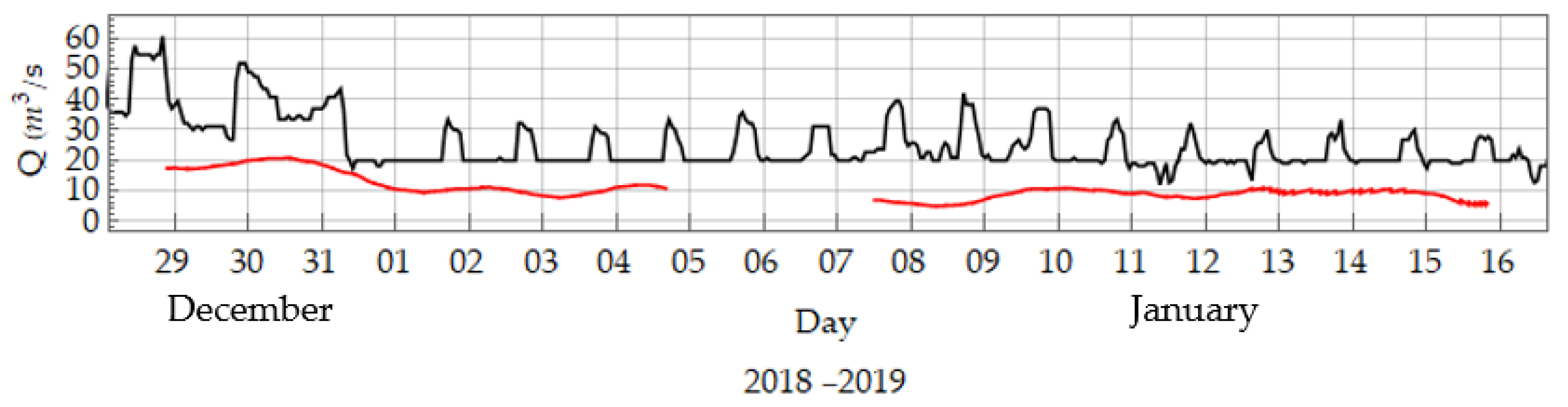
The freshwater runoff from the upstream of the Ōta River is regulated by an array of gates located near Gion Bridge. Under normal conditions only one gate is open. On regular days, the inflow discharge on the Ōta River is around 10–20% of the total flow rate [
20]. As shown in
Figure 7, the maximum freshwater runoff recorded at Yaguchi Gauging Station was 60 m
3/s in late 2018, which then declined to approximately 35 m
3/s in January 2019. Thus, the residual current at the study site was influenced almost exclusively by the upstream freshwater flow.
Error Analysis Results for the River Discharge Measurement
As mentioned in
Section 3.2, the deviations in FAT river discharge measurements may be estimated using Equation (9). Water depth and area are the functions of mean water depth (
H). The measurement errors of the water level loggers and the ADCP moving boat, as obtained from their specification manuals, are
= 0.01 m and
= 0.05 m, respectively. Water depths at the study site ranged from 1 m to 4 m. Hence, the uncertainty of the cross-sectional area ranged between 0.015 and 0.06.
In addition, the deviations in the velocity term deduced using FAT were
= 0.012 m/s, and the velocity along the three ray paths varied from −0.18 m/s to 0.4 m/s (
Figure 4). Thus, the measurement errors in the velocity resolution of FAT were 0.03–0.07.
The final term in the present case is attributable to the flow direction fluctuations and is given as . In this research, the angle between the streamline and the ray path was estimated using Equation (7), based on the velocities calculated by FAT. Because of the angle between the ray path and the streamline, the terms of discharge uncertainty were around ±0.045 for all three selected stations during the study period. Thus, the maximum probable error was estimated as 17.5%, which was considered acceptable.
4.4. Temporal Variations in Salinity Fluctuations
4.4.1. Longitudinal Salinity Distribution
The ability of the FAT system to accurately measure the salinity in a tidal estuary and monitor the salinity intrusion in a tidal floodway was demonstrated previously [
26,
27]. In previous research, CTD and FAT campaigns were conducted simultaneously to confirm the feasibility of using the FAT system to measure the section-average salinity.
As shown in
Figure 8a, the salinity deduced using FAT (black line) and Equation (5) was similar to the CTD estimates (blue points). The association between the salinity estimates obtained using FAT and Compact CTD, respectively, is illustrated in
Figure 8b. Both estimates show a similarity with a very high determination coefficient value (R
2 = 0.938), a bias of 0.275 psu, and low RMSE of 1.038 psu (4.325%). These observations provide further evidence that the FAT system is a reliable and accurate technique for the continuous monitoring of variations in salinity. In addition, the FAT dataset collected at three sections along the study site was used to calculate the section-average salinities, which were subsequently used to calculate the longitudinal distributions of salinity.
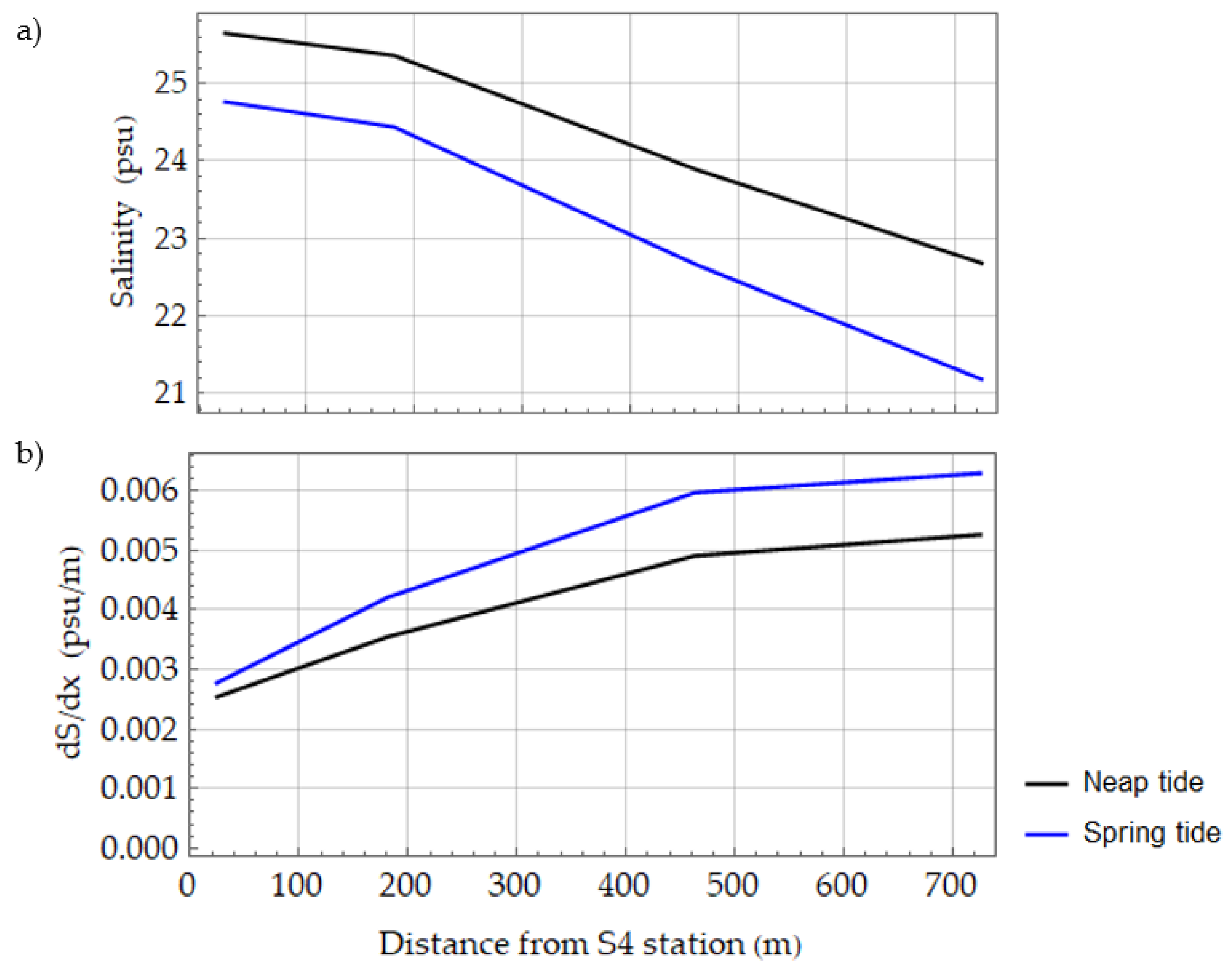
The longitudinal distributions of salinity and salinity gradient as deduced using the FAT system during a typical spring tide and a typical neap tide, respectively, are shown in
Figure 9.
In general, the depth-averaged salinity and the fluctuations in the salinity gradient followed opposite trend lines at the S4 station through the S1 station during both the spring and neap tides, with the former decreasing upward and the latter increasing upward.
As shown in
Figure 9, the average salinity value of the cross-sections showed a decline in the landward direction throughout the observation period, which was likely attributable to the impact of incoming freshwater.
The differences in cross-sectional average salinity between the downriver and upriver sections of the study site were found to be approximately 0.5–1.6 psu during spring tide and approximately 0.7–1.3 psu during neap tide. Moreover, the axial salinity during neap tide was approximately 0.5 psu higher than during spring tide, while the salinity gradients along the channel were lower during spring tide than neap tide. Therefore, at the study site, the variations in tidal salinity were significantly lower during spring tide, which may be explained by the different degrees of tidal mixing seen during the two tides, with the larger degree of tidal mixing that occurs during spring tides weakening the salt intrusion.
4.4.2. Longitudinal Dispersion Coefficient
The dispersion coefficient is used to quantify the local scattering of salt to adjacent areas. In this study, only the longitudinal dispersion coefficient was used, as longitudinal scales are generally larger than either transverse or vertical scales. Savenije [
28] stated that the salt intrusion process is ruled by three mechanisms, which include riverine–hydraulic dispersion, tide-driven dispersion, and gravitational circulation or density-driven dispersion.
As riverine–hydraulic dispersion is primarily influenced by geometric shapes and is small compared to tide- and density-driven dispersions, it may be eliminated [
27]. Other researchers have used other approaches (e.g., the longitudinal salt flux decomposition or the modelling approach) to verify which mechanisms are dominant in an estuary. In this research, the longitudinal dispersion coefficient deduced from the water velocity and salinity based on Equation (6) is discussed.
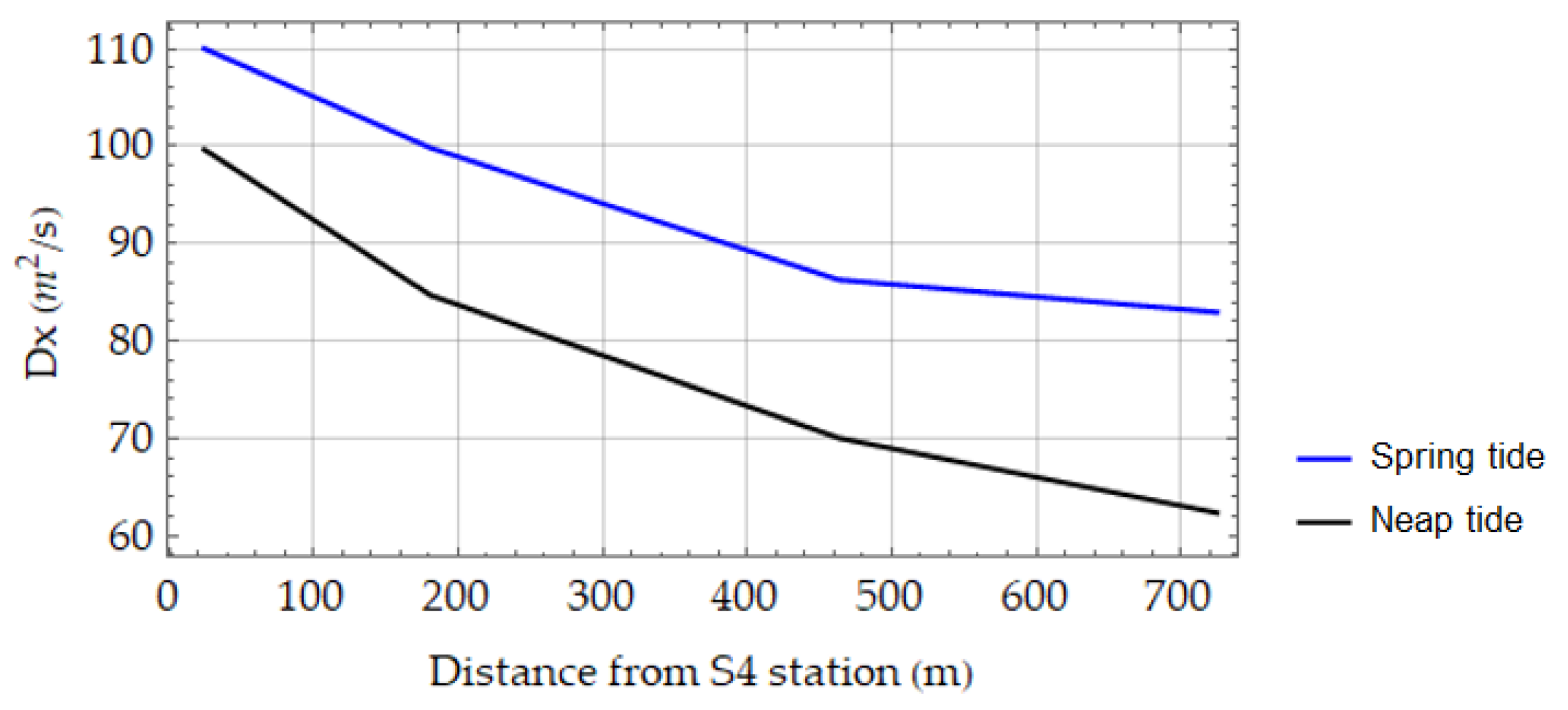
As shown in
Figure 10, the horizontal dispersion generates a relatively small dispersion coefficient upstream and a significantly increased coefficient downstream. In general, the dispersion coefficient depends primarily on the cross-sectional fluctuations in the velocity and salinity. In the Ōta channel, the change of cross-sectional velocity was found to increase slightly toward the mouth of the river (
Figure 4), and the axial salinity gradient was higher in the upstream section. As a result, the longitudinal dispersion coefficient increased as the distance to the mouth of the river decreased.
Soltaniasl et al. [
29] decomposed a cross-sectional salt flux into five different components and grouped these into two categories: landward fluxes and seaward fluxes. Although Soltaniasl et al. [
29] did not address the salt dispersion attributable to gravitational circulation due to the lack of related data, in this study, the total salt flux in the Ōta River estuary was found to be controlled significantly by the two categories, with the magnitude of the former category (landward fluxes) measuring half of the later (seaward fluxes). This result shows a significant effect of the tide on the salt flux in the Ōta channel. Furthermore, the Ōta channel is narrow and shallow, which is a state in which tide-driven shear mechanisms are often dominant [
28]. Thus, the tide-driven mechanism may be the dominant mechanism in the dispersion process in the Ōta channel.
4.5. Time Delays of Salinity Peaks
4.5.1. The Effect of Water Velocity on Travel Time/Salinity
The travel times,
tup and
tdown, at the upstream and downstream stations were estimated, respectively, using the following equations:
The components in Equation (11) are similar to those in Equations (1) and (2). The travel times in the upstream and downstream sections are not equal due to the direction of flow velocities (seaward or landward). Normally, the speed of sound, and thus salinity, is estimated using the mean travel time,
tm = (
tup +
tdown)/2. However, in cases where one of the travel times is missing,
tup or
tdown may be used to calculate the speed of sound, as the differences between travel times due to water velocity are small compared to the travel times. The travel time differences (
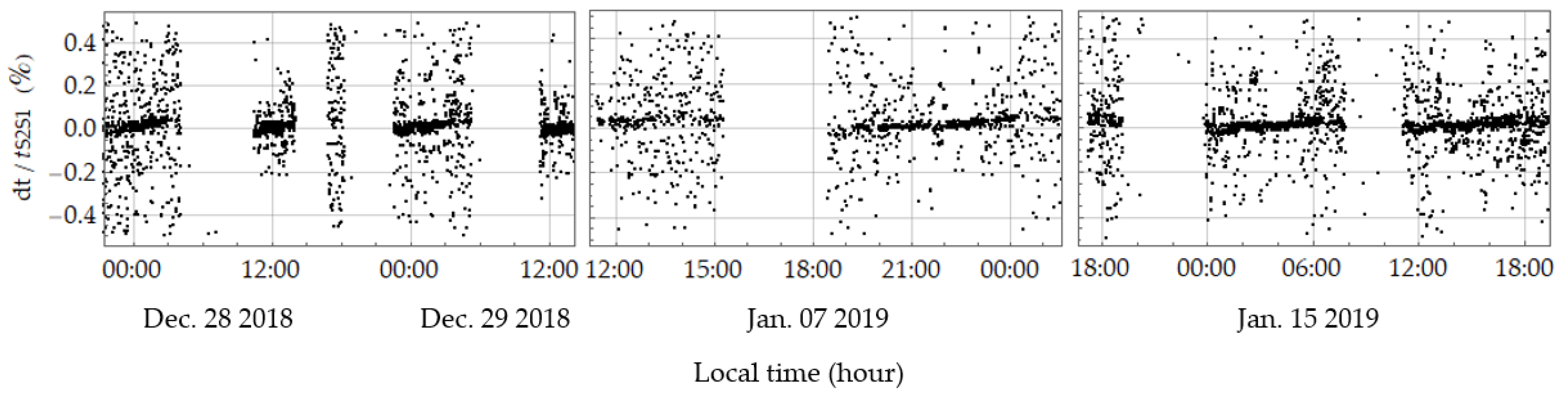
dt) compared to the travel time from S2 station to S1 station (
tS2S1) are presented in
Figure 11. The time shifts were small, and the maximum value was approximately 0.5%.
On the S1S2 transmission line, the sound transmitting data along the S1–S2 direction were more often lost than the data along the S2–S1 direction. Thus, the authors used the travel time data from the S2 station to the S1 station to calculate the salinity along the S1S2 section.
4.5.2. The Delays of Salinity Peaks
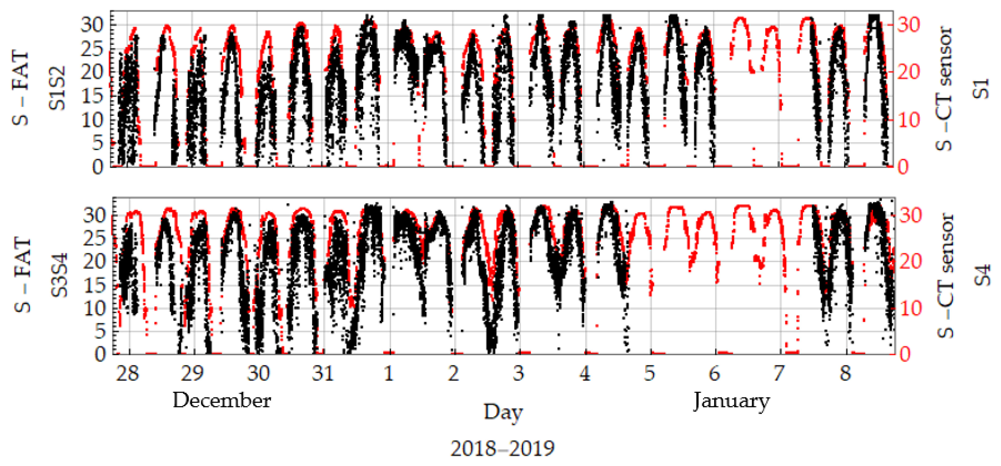
In
Figure 12, the black dots denote the temporal variations in the cross-sectional salinity that were estimated from the water temperature and the FAT data at two different cross-sections (S1S2 and S3S4), while red dots denote the salinity obtained by CT sensors deployed at the S1 and S4 stations. Compared to the stable trend of one-point salinities recorded at the S1 and S4 stations using a CT sensor, the section-averaged salinities deduced from the FAT data increased slightly at midday on 31 December 2018. The reason for these changes was that the water river discharge recorded at Yaguchi Station dropped significantly, halving after 31 December 2018. The time lags between the salinity maximum and the high water level were examined to clarify the effects of freshwater on the salinity.
Table 1 illustrates the time lags and phase lags between the salinity maximum and water level peak for further clarifications. Overall, it was evident that the time delay increased toward the mouth of the river, and the time shift changed significantly from before 31 December 2018 to after 31 December 2018.
First of all, the time delay estimated in the downstream area (S3S4 section) was twice as high as the time delay in the upstream area (S1S2 section) over the study period. Moreover, the delay in the salinity maximum along the channel ranged from 12 min to approximately 1.5 h. All three sections of the channel showed significantly higher time delays after 31 December 2018 than before this date. These delays were likely due to the noticeable decrease in freshwater discharge recorded at Yaguchi Station in the upstream section of the river after that day (
Figure 7).
In general, the delays found at the time of the salinity peaks were likely attributable to density current effects and cross-channel processes such as changes in water depth, differences in vertical velocities (both values and direction), and secondary flows [
30]. In this research, the phase lags noted between the water level and salinity exist primarily because of the freshwater flows from the upstream and the inflow of seawater flows from the Old Ōta River in the same Ōta River system [
26].
5. Conclusions
The longitudinal distribution of intra-tidal changes in the velocity/discharge and salinity in the middle part of a diversion channel was monitored in this study. Velocity was measured concurrently using the FAT system and a moving-boat Stream–Pro ADCP. The section-average speed of sound was measured by placing four acoustic stations installed along the site study located on the broadest branch of the Ōta River system. The salinity could be deduced from the water temperature, water depth, and the speed of sound from FAT using Medwin’s formula. The main conclusions of this study are summarized below:
The differences in the section-average velocities obtained using FAT and ADCP were not significant. Moreover, the cross-sectional mean salinity derived using the FAT system was acceptably similar to the results obtained using the Compact CTD.
The studied section of the river exhibited asymmetric ebb-tide and flood-tide velocities, with a short-duration ebb phase of the tide and fast ebb currents that created an ebb-dominant phenomenon, which was likely due to the topographic effects and river runoff.
The residual current resembled density-driven circulation and was affected primarily by the freshwater discharge from upstream.
The section-average salinity increased seaward, revealing typical estuarine behavior. In addition, the salinity pattern revealed a completely tide-dominated influence. Furthermore, the delays in time between the salinity maximum and high water level were observed, with the duration of the delay increasing downstream, due primarily to density current effects.
The longitudinal dispersion coefficient was found to increase toward the mouth of the river. The Ōta channel is a narrow and shallow channel which can cause dominant, tide-driven shear mechanisms. Thus, the tide-driven mechanism may be the dominant mechanism in the dispersion process in the Ōta channel.
The Ōta River estuary, with other branches of the Ōta River system, is located inside Hiroshima Bay, bordered by a complicated coastline. The coastal dynamic conditions of Hiroshima Bay affect the dynamic process of each estuary; in return, the general estuarine dynamic of these estuaries could influence the dynamic conditions of Hiroshima Bay. Thus, further investigation of the 2D salinity distribution in Hiroshima Bay, together with other modern techniques such as remote sensing, is highly recommended to further understand the estuarine dynamic of the Ōta River estuary.
Finally, this study presents the detailed results of using a novel and promising method of continuous salinity and velocity distribution monitoring along a tidal channel.
Author Contributions
H.T.N.: Conceptualization, Methodology, Software, Data curation, Writing—Original draft preparation. K.K.: Supervision, Methodology, Validation, Reviewing and Editing, Validation, Original draft revision. M.B.A.S.: Writing—review and editing. All authors have read and agreed to the published version of the manuscript.
Funding
This research received no external funding.
Institutional Review Board Statement
Not applicable.
Informed Consent Statement
Not applicable.
Data Availability Statement
Streamflow data as computed was provided by the Ministry of Land Infrastructure Transport (MLIT), Japan. The QFAT data from this study are available from the corresponding author upon request.
Conflicts of Interest
The authors declare no conflict of interest.
Appendix A
The detailed equation of the relative errors of flow direction estimation:
where:
References
- Laenen, A.; Smith, W. Acoustic Systems for the Measurement of Streamflow; Open-File Report 82-329; U.S. Geological Survey: Reston, VA, USA, 1982. [Google Scholar] [CrossRef]
- Prandle, D. Dynamical Controls on Estuarine Bathymetry: Assessment against UK Database. Estuar. Coast. Shelf Sci. 2006, 68, 282–288. [Google Scholar] [CrossRef]
- Chen, Q.; Zhu, J.; Lyu, H.; Pan, S.; Chen, S. Impacts of Topography Change on Saltwater Intrusion over the past Decade in the Changjiang Estuary. Estuar. Coast. Shelf Sci. 2019, 231, 106469. [Google Scholar] [CrossRef]
- Li, L.; Zhu, J.; Wu, H. Impacts of Wind Stress on Saltwater Intrusion in the Yangtze Estuary. China Earth Sci. 2012, 55, 1178–1192. [Google Scholar] [CrossRef]
- Garel, E.; D’Alimonte, D. Continuous River Discharge Monitoring with Bottom-mounted Current Profilers at Narrow Tidal Estuaries. Cont. Shelf Res. 2016, 133, 1–12. [Google Scholar] [CrossRef]
- Kawanisi, K.; Bahrainimotlagh, M.; Al Sawaf, M.B.; Razaz, M. High-frequency Streamflow Acquisition and Bed Level/flow Angle Estimates in a Mountainous River Using Shallow-water Acoustic Tomography. Hydrol. Process. 2016, 30, 2247–2254. [Google Scholar] [CrossRef]
- Maghrebi, M.F.; Ahmadi, A.; Attari, M.; Maghrebi, R.F. New Method for Estimation of Stage-discharge Curves in Natural Rivers. Flow Meas. Instrum. 2016, 52, 67–76. [Google Scholar] [CrossRef]
- Geawhari, M.A.; Huff, L.; Mhammdi, N.; Trakadas, A.; Ammar, A. Spatial-temporal Distribution of Salinity and Temperature in the Oued Loukkos Estuary, Morocco: Using Vertical Salinity Gradient for Estuary Classification. SpringerPlus 2014, 3, 1–9. [Google Scholar] [CrossRef] [PubMed] [Green Version]
- McManus, J. Salinity and Suspended Matter Variations in the Tay Estuary. Cont. Shelf Res. 2005, 25, 729–747. [Google Scholar] [CrossRef]
- Dyer, K.R.; Gong, W.K.; Ong, J.E. The Cross Sectional Salt Balance in a Tropical Estuary during a Lunar Tide and a Discharge Event. Estuar. Coast. Shelf Sci. 1992, 34, 579–591. [Google Scholar] [CrossRef]
- Vaz, N.; Dias, J.M.; Leitão, P.; Martins, I. Horizontal Patterns of Water Temperature and Salinity in an Estuarine Tidal Channel: Ria de Aveiro. Ocean Dyn. 2005, 55, 416–429. [Google Scholar] [CrossRef] [Green Version]
- Yi, D.; Melnichenko, O.; Hacker, P. Remote Sensing of Sea Surface Salinity Variability in the South China Sea. J. Geophys. Res. Ocean. 2020, 125, 1–24. [Google Scholar] [CrossRef]
- Klemas, V. Remote Sensing of Sea Surface Salinity: An overview with Case Studies. J. Coast. Res. 2011, 27, 830–838. [Google Scholar] [CrossRef]
- Kawanisi, K.; Al Sawaf, M.B.; Danial, M.M. Automated Real-time Stream Flow Acquisition in a Mountainous River Using Acoustic Tomography. J. Hydrol. Eng. 2018, 23, 04017059. [Google Scholar] [CrossRef]
- Bahreinimotlagh, M.; Kawanisi, K.; Danial, M.M.; Al Sawaf, M.B.; Kagami, J. Application of Shallow-water Acoustic Tomography to Measure Flow Direction and River Discharge. Flow Meas. Instrum. 2016, 51, 30–39. [Google Scholar] [CrossRef]
- Razaz, M.; Kawanisi, K.; Kaneko, A.; Nistor, I. Application of Acoustic Tomography to Reconstruct the Horizontal Flow Velocity Field in a Shallow River. Water Resour. Res. 2015, 51, 9665–9678. [Google Scholar] [CrossRef] [Green Version]
- Al Sawaf, M.B.; Kawanisi, K.; Xiao, C. Measuring Low Flowrates of a Shallow Mountainous River Within Restricted Site Conditions and the Characteristics of Acoustic Arrival Times Within Low Flows. Water Resour. Manag. 2020, 34, 3059–3078. [Google Scholar] [CrossRef]
- Razaz, M.; Kawanisi, K.; Nistor, I.; Rennie, C. Continuous Velocity Measurement with Travel-time Method in Stratified Shallow Flows. In Proceedings of the 1st International Conference and Exhibition on Underwater Acoustics, Corfu, Greece, 23–28 June 2013; pp. 555–562. [Google Scholar]
- Danial, M.M.; Kawanisi, K.; Al Sawaf, M.B. Characteristics of Tidal Discharge and Phase Difference at a Tidal Channel Junction Investigated Using the Fluvial Acoustic Tomography System. Water 2019, 11, 857. [Google Scholar] [CrossRef] [Green Version]
- Kawanisi, K.; Razaz, M.; Kaneko, A.; Watanabe, S. Long-term Measurement of Stream Flow and Salinity in a Tidal River by the Use of the Fluvial AcousticTomography System. J. Hydrol. 2010, 380, 74–81. [Google Scholar] [CrossRef]
- Medwin, H. Speed of sound in water: A Simple Equation for Realistic Parameters. J. Acoust. Soc. Am. 1975, 58, 1318–1319. [Google Scholar] [CrossRef]
- Boon, J.D.; Byrne, R.J. On Basin Hypsometry and the Morphodynamic Response of Coastal Inlet Systems. Mar. Geol. 1981, 40, 27–48. [Google Scholar] [CrossRef]
- Fitzgerald, D.M.; Nummedal, D. Response Characteristics of an Ebb-dominated Tidal Inlet Channel. J. Sediment. Petrol. 1983, 53, 833–845. [Google Scholar]
- Wolf, J.; Prandle, D. Some observations of wave-current interaction. Coast. Eng. 1999, 37, 471–485. [Google Scholar] [CrossRef]
- Soulsby, R.L.; Hamm, L.; Klopman, G.; Myrhaug, D.; Simons, R.R.; Thomas, G.P. Wave-current interaction within and outside the bottom boundary layer. Coast. Eng. 1993, 21, 41–69. [Google Scholar] [CrossRef]
- Kawanisi, K.; Razaz, M.; Soltaniasl, M.; Kaneko, A. Long-Term Salinity Measurement in a Tidal Estuary by the Use of Acoustic Tomography. In Proceedings of the 4th International Conference and Exhibition on “Underwater Acoustics Measurements: Technologies & Results”, Kos Island, Greece, 20–24 June 2011; pp. 401–408. [Google Scholar]
- Kawanisi, K.; Razaz, M.; Motlagh, M.B. Monitoring Flow Rate and Salinity Intrusion in a Tidal Floodway Using Fluvial Acoustic Tomography. In Proceedings of the 36th IAHR World Congress, The Hague, The Netherlands, 28 June–3 July 2015; pp. 6634–6641. [Google Scholar]
- Savenije, H.H.G. Composition and driving mechanisms of longitudinal tidal average salinity dispersion in estuaries. J. Hydrol. 1993, 144, 127–141. [Google Scholar] [CrossRef]
- Soltaniasl, M.; Kawanisi, K.; Yano, J.; Ishikawa, K. Variability in salt flux and water circulation in Ota River Estuary, Japan. Water Sci. Eng. 2013, 6, 283–295. [Google Scholar]
- Dyer, K.R. Estuaries: A Physical Introduction, 2nd ed.; Wiley: New York, NY, USA, 1997; pp. 33–37. [Google Scholar]
Figure 1.
(a) The location of the field observation at the Ōta River Estuary; (b) the arrangement of the tomographic scheme of the FAT system over the Ōta River. Yellow and purple symbols indicate the locations of the CT instruments; and (c) the Compact CTD (yellow circles) and FAT (red triangles) campaigns for validating section-average salinity using the FAT system.
Figure 2.
Oblique cross-sections along transmission lines between S1–S2, S2–S3, and S3–S4. Dashed lines denote the Highest Water Level (HWL) and the Lowest Water Level (LWL), and black dots denote the placed transducers.
Figure 2.
Oblique cross-sections along transmission lines between S1–S2, S2–S3, and S3–S4. Dashed lines denote the Highest Water Level (HWL) and the Lowest Water Level (LWL), and black dots denote the placed transducers.
Figure 3.
Temporal variations of water level during the study period recorded at the observed cross-sections.
Figure 3.
Temporal variations of water level during the study period recorded at the observed cross-sections.
Figure 4.
Time series for the tidal current velocities (black) and the residual mean velocity (red) measured using FAT at the selected stations during the study period.
Figure 4.
Time series for the tidal current velocities (black) and the residual mean velocity (red) measured using FAT at the selected stations during the study period.
Figure 5.
Temporal variations in water discharge (black) and residual flow (red) estimated using FAT at the selected stations during the study period.
Figure 5.
Temporal variations in water discharge (black) and residual flow (red) estimated using FAT at the selected stations during the study period.
Figure 6.
(a) Comparison of the discharges acquired using the FAT (black) and ADCP (blue) and (b) The association between the FAT and ADCP estimates.
Figure 6.
(a) Comparison of the discharges acquired using the FAT (black) and ADCP (blue) and (b) The association between the FAT and ADCP estimates.
Figure 7.
Comparison of the freshwater release from the Yaguchi Station (black) and the residual discharge as estimated using FAT (red).
Figure 7.
Comparison of the freshwater release from the Yaguchi Station (black) and the residual discharge as estimated using FAT (red).
Figure 8.
(a) Water level at Gion Gauging Station (red line), and the comparison between the salinity acquired using FAT (black line) and Compact CTD (blue dots) at Shinkoi Bridge, (b) The association between the FAT and Compact CTD estimates, and (c) Vertical salinity profile obtained using Compact CTD.
Figure 9.
Longitudinal distributions of salinity (a) and salinity gradient (b) deduced using the FAT system during spring tide and neap tide.
Figure 9.
Longitudinal distributions of salinity (a) and salinity gradient (b) deduced using the FAT system during spring tide and neap tide.
Figure 10.
Longitudinal distributions of the dispersion coefficient deduced using the FAT system during spring tide and neap tide.
Figure 10.
Longitudinal distributions of the dispersion coefficient deduced using the FAT system during spring tide and neap tide.
Figure 11.
The travel time differences compared to travel time from S2 station to S1 station.
Figure 11.
The travel time differences compared to travel time from S2 station to S1 station.
Figure 12.
Temporal variation of salinity obtained using FAT (black points) at S1S2 and S3S4 transmission lines and CT sensors (red points) at S1 and S4 stations.
Figure 12.
Temporal variation of salinity obtained using FAT (black points) at S1S2 and S3S4 transmission lines and CT sensors (red points) at S1 and S4 stations.
Table 1.
Delays in time of salinity peaks.
Table 1.
Delays in time of salinity peaks.
| | S1S2 Section | S2S3 Section | S3S4 Section |
|---|
| Peak Number | Time Lag (min) | Phase Lag (°) | Time Lag (min) | Phase Lag (°) | Time Lag (min) | Phase Lag (°) |
|---|
| Before 31 December 2018 |
| 1 | 14 | 6.73 | 17 | 8.17 | 28 | 13.46 |
| 2 | 21 | 10.10 | 27 | 12.98 | 37 | 17.79 |
| 3 | 15 | 7.21 | 24 | 11.54 | 31 | 14.90 |
| 4 | 12 | 5.77 | 24 | 11.54 | 36 | 17.31 |
| 5 | 16 | 7.69 | 26 | 12.50 | 40 | 19.23 |
| After 31 December 2018 |
| 1 | 22 | 10.58 | 31 | 14.90 | 87 | 41.83 |
| 2 | 32 | 15.38 | 26 | 12.50 | 94 | 45.19 |
| 3 | 23 | 11.06 | 42 | 20.19 | 91 | 43.75 |
| 4 | 21 | 10.10 | 38 | 18.27 | 55 | 26.44 |
| 5 | 23 | 11.06 | 37 | 17.79 | 97 | 46.63 |
| Publisher’s Note: MDPI stays neutral with regard to jurisdictional claims in published maps and institutional affiliations. |
© 2021 by the authors. Licensee MDPI, Basel, Switzerland. This article is an open access article distributed under the terms and conditions of the Creative Commons Attribution (CC BY) license (https://creativecommons.org/licenses/by/4.0/).


