Motion of Floating Caisson with Extended Bottom Slab under Regular and Irregular Waves

Abstract

Floating caissons may oscillate primarily due to ocean waves during towing operations. Reducing the oscillation based on the extension part (footing) of the bottom slab of the caissons can efficiently increase the safety of towing maneuvers. However, the influence of the footing length on the motion of floating caissons has not been adequately studied. This study investigates this topic through hydraulic model experiments and numerical simulations. Experimental results for regular waves show that the rotational motion (pitch) of the caisson around the wave crest direction increases owing to resonance. This suggests that the pitch could be reduced by designing caissons, such that resonance may be prevented along the footing length. In the numerical simulations of irregular waves, the Fourier amplitudes of the heave and pitch show that the footings amplify their low-frequency components and reduce their high-frequency components. Furthermore, the significant total amplitudes of the heave and pitch show a different trend from that of the regular waves observed in the hydraulic model experiments. This suggests that it is essential to examine the motion of a caisson under irregular waves when assessing the effect of footings in an actual marine environment.

1. Introduction

Caissons are essentially large hollow boxes made of reinforced concrete and are used as coastal and harbor structures, such as breakwaters, quay walls, and bridge piers. Such caissons are typically built on land yards, dry docks, and floating docks. The completed caisson is floated in the sea and towed to a construction site using tugboats. At the final position of the caisson, sea water is poured into the caisson, and the caisson is settled on the rubble mound. Subsequently, crushed stone is placed inside the caisson, and finally, cap concrete is constructed on the caisson. An example of the design, construction, and installation of caissons used as bridge piers was reported by Chakrabarti et al. [1].

When towing a floating caisson, it may significantly oscillate depending on the wave conditions. To increase the safety of towing maneuvers and the availability of construction works, it is necessary to reduce the oscillation of a floating caisson. Huang et al. [2] examined the responses of a free-floating rectangular caisson from hydraulic model experiments and numerical simulations using a frequency-domain solver, WAMIT, and a time-domain solver, Star-CCM+. The numerical results have shown that the drift velocity of the caisson is several times larger than the Stokes drift velocity. Huang et al. [3] experimentally investigated a cable system and an anchor system for positioning and installing a large caisson. This study showed the acceptable wave conditions when using the cable system and the appropriate drafts of the caisson when using the anchor cable system. Kotake et al. [4] focused on the motion of a small caisson hung with crane wires. Based on numerical simulations using a three-dimensional coupled fluid–structure–sediment–seabed interaction model (FS3M) [5], this study showed that minimizing the quantity of water inside the caisson and subsequently decreasing the draft of the caisson was effective in reducing the oscillation of the caisson under predetermined wave conditions. Meneses et al. [6] developed a new dynamic positioning control system for the sinking process of floating caissons and implemented it in an experimental test campaign. This study demonstrated the possibility of dynamically controlling the horizontal position of a floating caisson during the sinking phase to increase the safety and success of the positioning and sinking maneuvers. Gu et al. [7] evaluated the motion of a towed caisson under combined wind and wave fields using Ansys AQWA. Regarding the heave (vertical translational motion) of the caisson, this study has shown that the maximum value is affected by the towrope length and draft, and the fluctuation is influenced by the towing speed and draft.

In general, the bottom slab of a caisson overhangs the offshore and onshore sides to reduce the contact pressure acting on the foundation and enhance the stability of the caisson. This extension part of the bottom slab is referred to as “footing” in this study. Using such footings to reduce the oscillation of a floating caisson could prove efficient. Nagasawa et al. [8] conducted hydraulic model experiments focusing on the motion of floating caissons with different footing lengths and found that the significant value of the heave under irregular waves decreases with an increase in the footing length. From numerical simulations based on the source technique, Ishimi et al. [9] showed that footings reduce the heave and pitch (rotational motion around the wave crest direction). Michimae et al. [10] experimentally revealed that the pitch of a floating long caisson with a non-rectangular shape is small in the presence of footings compared with caissons without footings. However, there is no study that has varied the footing length except for Nagasawa et al. [8], and their investigation was limited to the influence on the heave. Hence, the mechanism of the influence of the footing length on the motion of a floating caisson is not clearly understood.

In this study, the characteristics and mechanism of the motion of a floating caisson were investigated by changing the footing length through hydraulic model experiments and numerical analyses. Free and forced oscillation experiments were conducted in the hydraulic model experiments. In the free oscillation experiments, the natural frequency of the caisson was obtained by oscillating the caisson under still-water conditions. In the forced oscillation experiments, regular waves were generated toward the caisson with different footing lengths to determine the motion of the caisson. In the numerical analyses, simulations modeled based on the hydraulic model experiments were conducted for free and forced oscillation simulations using the three-dimensional coupled fluid–structure–sediment–seabed interaction model (FS3M) [5]. In the free oscillation simulations, the natural frequency of the caisson was computed by oscillating the caisson under still-water conditions and comparing the results with experimental data. In the forced oscillation simulations, the caisson was subjected to regular and irregular waves. For the regular waves, the predictive capability of FS3M was demonstrated through comparison with experimental results. For the irregular waves, the motion of the caisson was investigated to assess the effect of footings in an actual marine environment.

The rest of the present paper is organized as follows: Chapter 2 describes the setup and conditions in the hydraulic model experiments. Subsequently, experimental data are presented and discussed in Chapter 3. Chapter 4 gives a brief explanation of FS3M for completeness and describes the computational setup and conditions in the numerical analyses. In Chapter 5, numerical results are presented and discussed through a comparison with the experimental data. Finally, conclusions are summarized in Chapter 5.

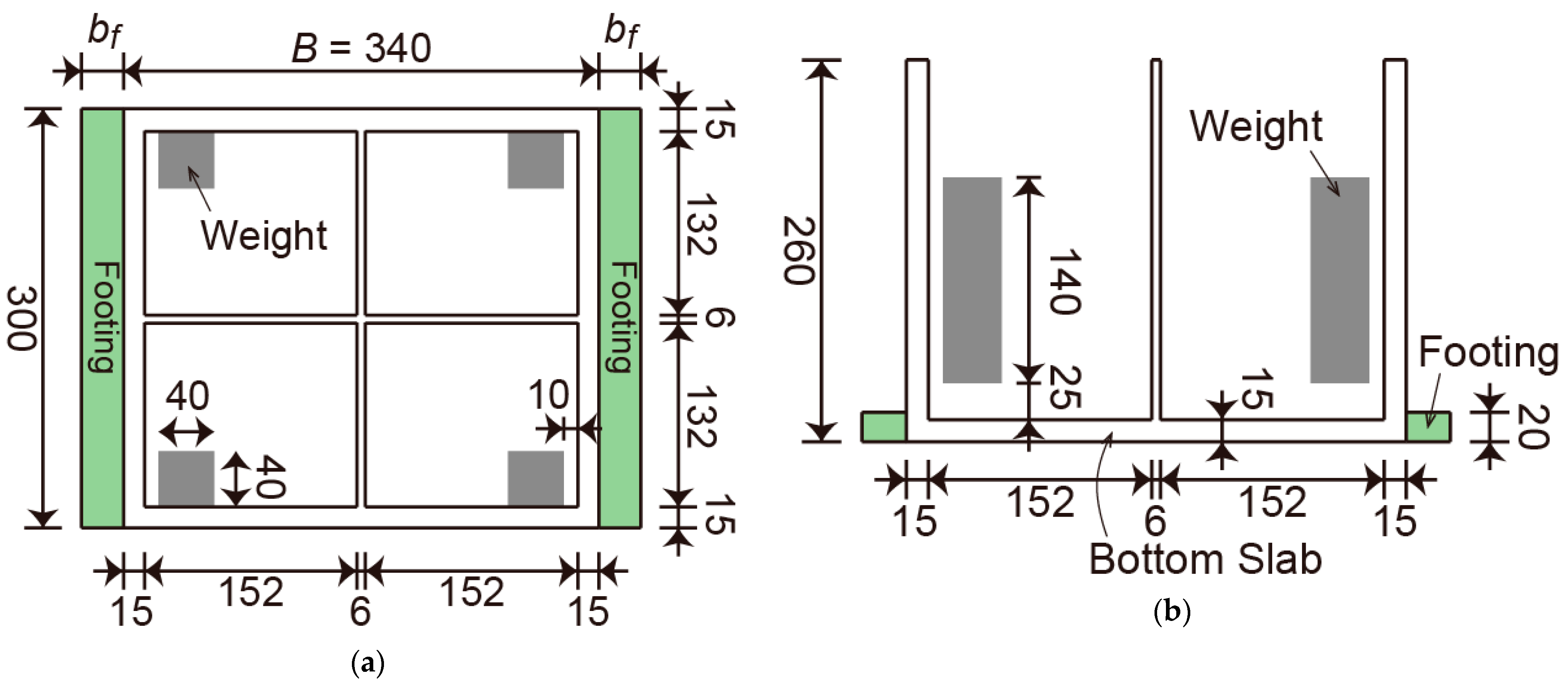
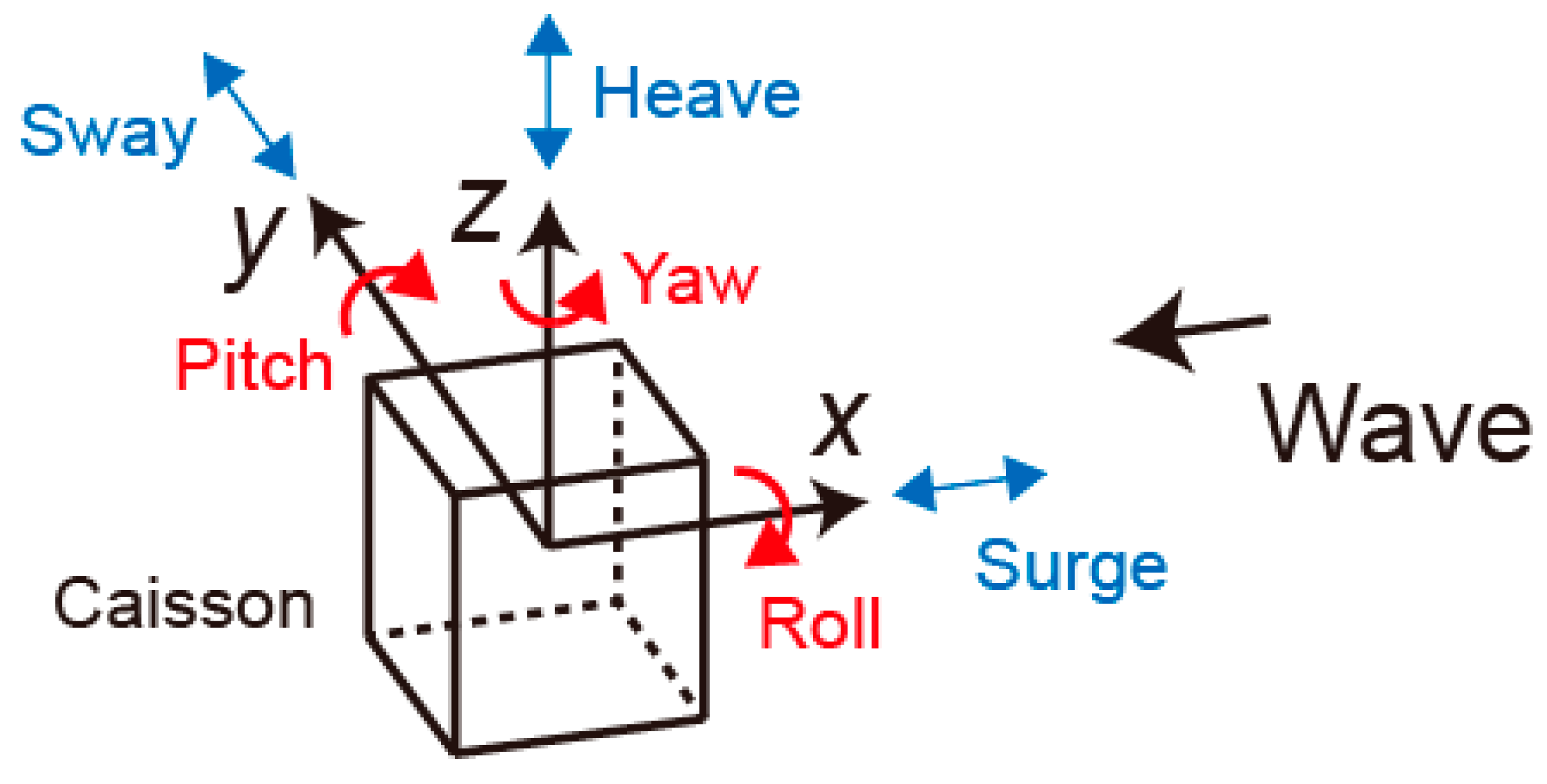
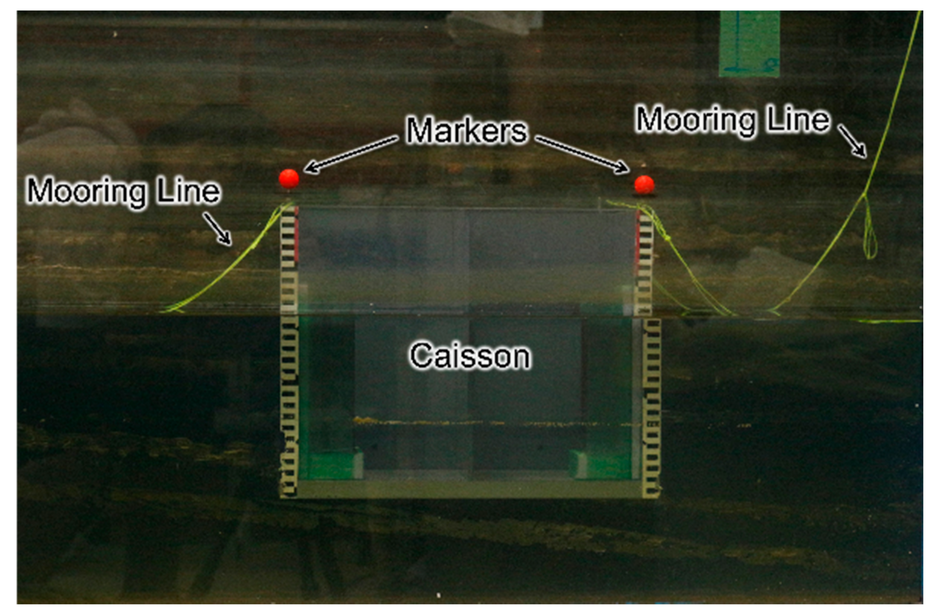
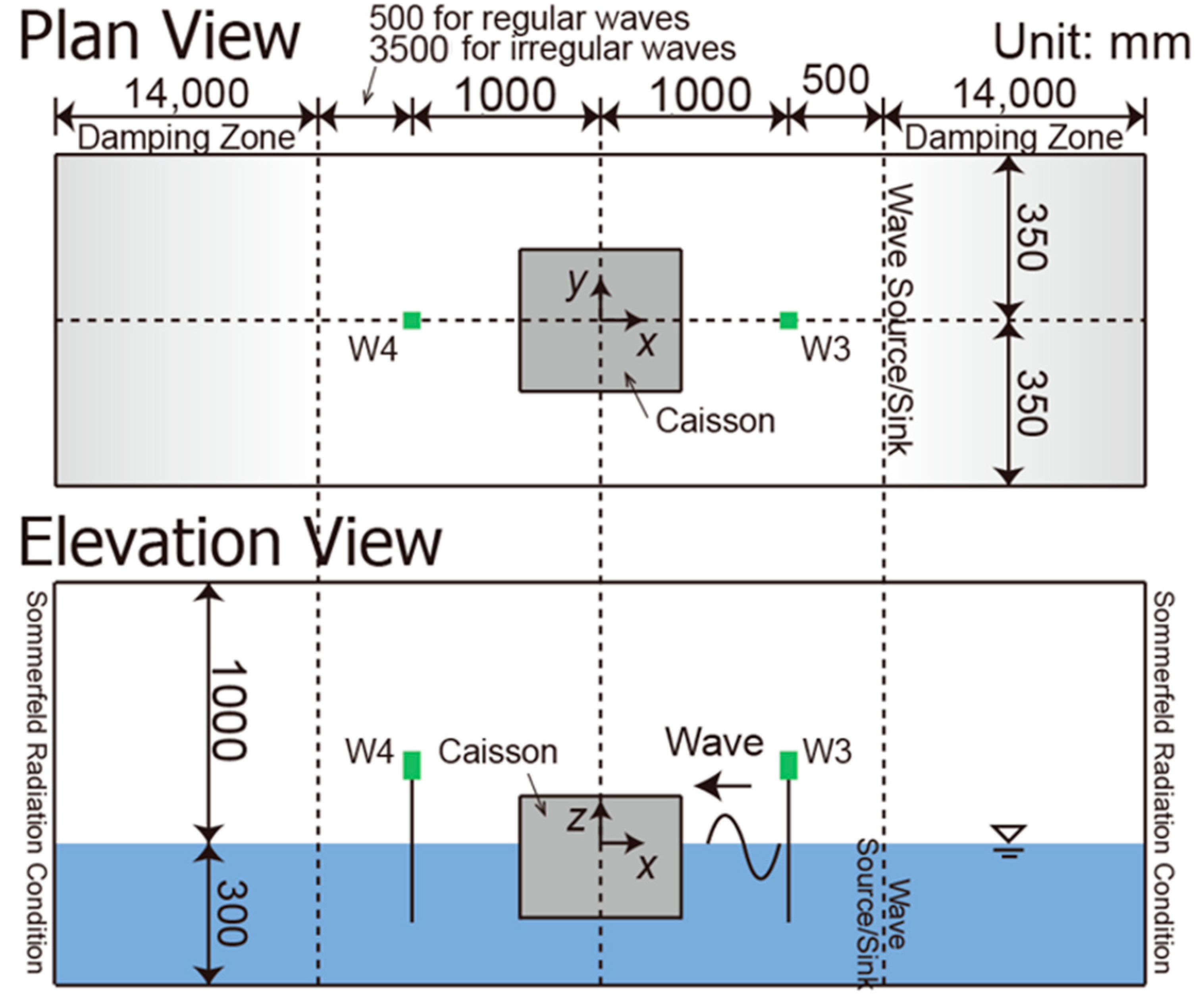
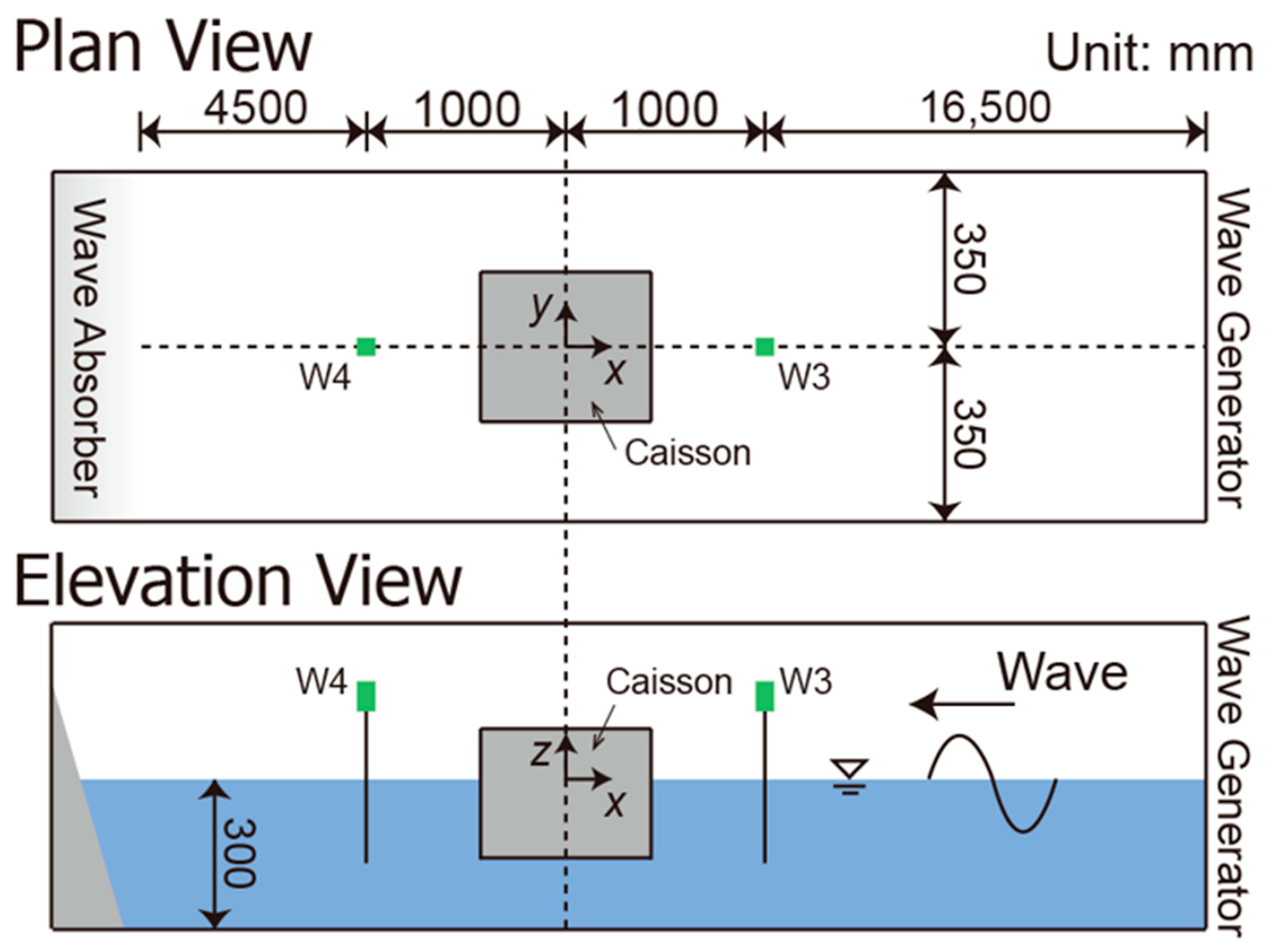
2. Experimental Setup and Conditions

A series of hydraulic model experiments were conducted at a length scale of 1/50 based on the Froude similarity law, using a 30.0-m-long, 0.7-m-wide, and 0.90-m-high wave flume equipped with a piston-type wave generator (Fudo Tetra Co., Tokyo, Japan) in Nagoya University, Japan. Since an active wave absorption system in the wave generator was not used in this study, the wave paddle was displaced sinusoidally following the linear wave theory. A wave absorber, which was composed of a gravel beach covered with a polypropylene filter material, was set at the other end of the flume.

The schematic of the experimental setup is shown in Figure 1. The schematic and specifications of a modeled 20-ton rectangular caisson are presented in Figure 2 and

Table 1. Specifications of the caisson without the footings.

	Model Scale (1/50)	Prototype Scale
Length B	0.34 m	17.0 m
Height	0.26 m	13.0 m
Width	0.30 m	15.0 m
Mass	16.8 kg	2100 t
Draft	0.16 m	8.0 m
Height of Gravity Center	0.108 m	5.4 m

. As shown in Figure 2 and Table 1, the caisson was made of polyvinyl chloride (PVC) with a x-directional length B of 0.34 m, a y—directional width of 0.30 m, and a z-directional height of 0.26 m. The steel weights shown in gray in Figure 2 were used to adjust the mass to 16.8 kg, the draft to 0.16 m, and the height of the gravity center from the bottom to 0.108 m. The position and weight of the weights were determined to match the mass and moment of inertia with the prototype. The specifications of the footings are presented in

Table 2. Specifications of the footings.

	Model Scale (1/50)	Prototype Scale
Height	0.02 m	1.0 m
Length bf	0.00 m	0.0 m
	0.02 m	1.0 m
	0.03 m	1.5 m
	0.04 m	2.0 m
	0.06 m	3.0 m

. The footings were made of PVC, the z—directional height of the footings was set to 0.02 m based on the prototype caisson, and the x—directional length of the footings b_f was changed to 0.00 (no footing), 0.02, 0.03, 0.04, and 0.06 m. The caisson with and without the footings was floated in the wave flume with a still water depth of 0.30 m, as shown in Figure 1.

Two light markers were attached to the top of the caisson, and the videos of the caisson with the markers were recorded using a high-speed camera (DITECT Co. Ltd., Tokyo, Japan, HAS-L1). From the videos, the surge, heave, and pitch at the gravity center of the caisson defined in Figure 3 were calculated using DIPP-Motion V/3D (DITECT Co. Ltd.). To prevent the caisson from moving largely in the surge direction and hitting the wave gauges, the caisson was loosely moored using light, thin threads such that its motions were not affected. Figure 4 shows the initial state of the caisson and mooring lines. Capacitance-type wave gauges (KENEK Co. Ltd., Tokyo, Japan, CHT6-40) were installed at W3 and W4 (see Figure 1) to measure the water surface fluctuations.

Free and forced oscillation experiments were performed. In the free oscillation experiments, the caisson floating under the still-water condition was lifted a few centimeters upward from both sides or one side and released to facilitate free motion in the heave or pitch direction. To confirm the reproducibility, three experimental runs were conducted for each case. In the forced oscillation experiments, as shown in

Table 3. Incident regular waves used in the forced oscillation experiments.

Still Water Depth h [m]	Wave Height Hi [m]	Wave Frequency fi [Hz]	Goda’s Nonlinear Parameter Π
0.30	0.03	0.88	0.033
0.30	0.03	0.59	0.051
0.30	0.03	0.44	0.079
0.30	0.03	0.35	0.117
0.30	0.03	0.29	0.163
0.30	0.03	0.25	0.218

, regular waves with an incident wave height of H_i = 0.03 m and an incident wave period of T_i = 1.13, 1.70, 2.26, 2.83, 3.39, and 3.96 s were generated toward the floating caisson. In the table, f_i is the incident wave frequency, and Π is Goda’s nonlinear parameter (Π=H_i/L_i coth³ 2πh/L_i; L_i: wavelength) [11]. The wave period T_i was determined assuming a port on the Pacific coast of Japan. The stroke of the wave paddle was determined for each wave period from incident wave heights measured without the caisson to obtain the specific wave height.

3. Experimental Results and Discussion

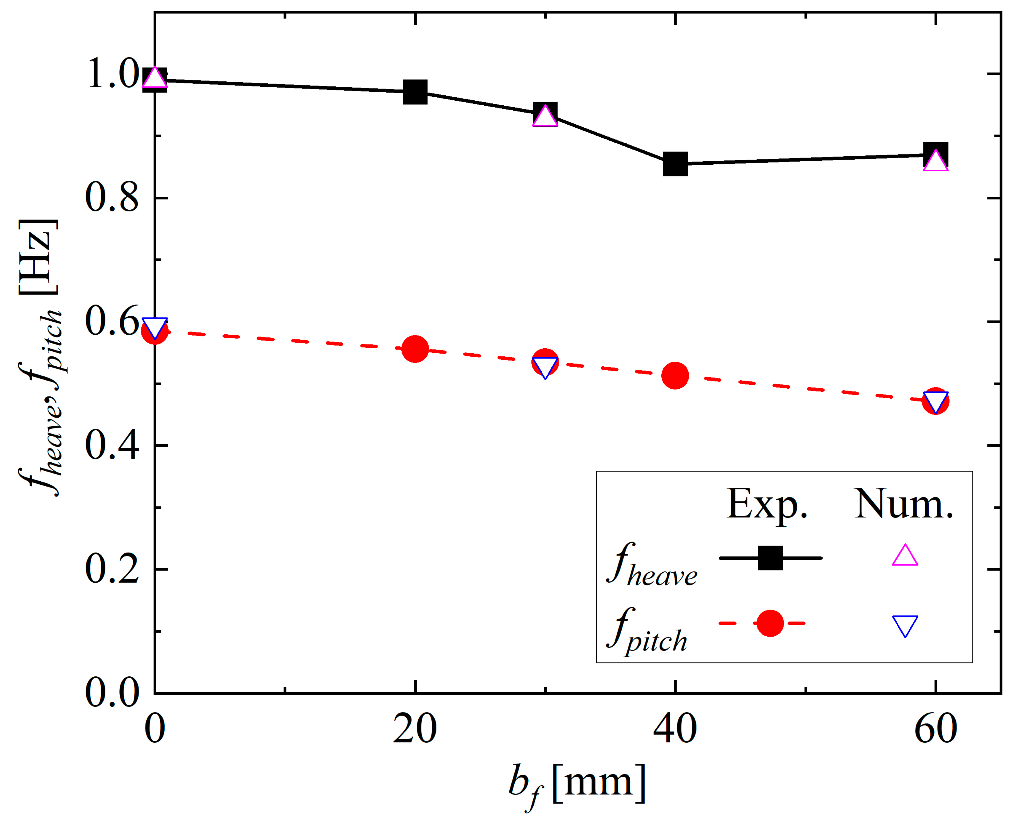
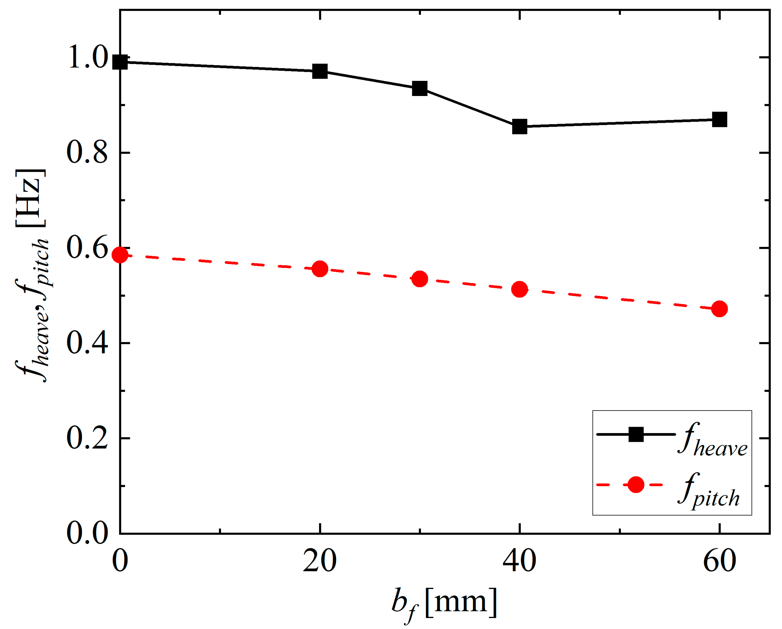
3.1. Natural Frequency

Figure 5 shows the natural frequencies of the heave f_heave and pitch f_pitch obtained from the free oscillation experiments. Here, f_heave and f_pitch are the average values of the three experimental runs. The maximum variabilities of the three experimental runs with respect to the average values were 9.4% for f_heave and 1.4% for f_pitch. From Figure 5, the natural frequency of the heave f_heave (black solid line) tends to decrease with an increase in the footing length b_f. Similarly, the natural frequency of the pitch f_pitch (red broken line) tends to decrease linearly as the footing length b_f increases. The longer the footings, the larger the water mass above and under the footings that must be moved. This slows the motion of the caisson; hence, f_heave and f_pitch decrease with an increase in b_f.

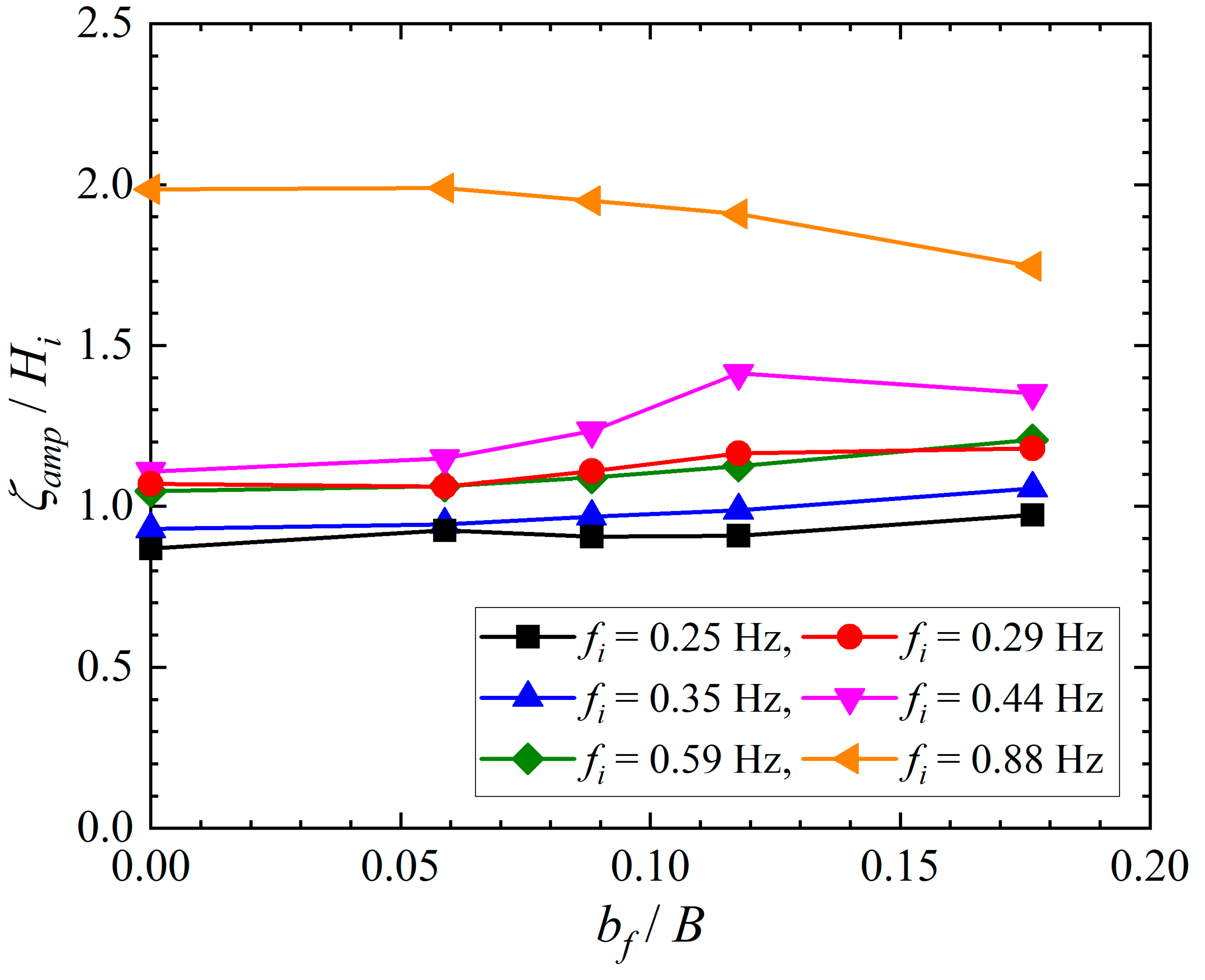
3.2. Total Amplitude of Heave

Figure 6 shows the relationship between the normalized values of the total amplitude of the heave ζ_amp and those of the footing length b_f, where ζ_amp is the three-period average of the difference between the maximum and minimum values of the heave. From the figure, the change in ζ_amp/H_i with the relative footing length b_f/B depends on the incident wave frequency f_i. For f_i = 0.29, 0.35, and 0.59 Hz (red, blue, and green lines), the value of ζ_amp/H_i slightly increases with b_f/B. In contrast, the cases of f_i = 0.88 Hz (orange line) show that the value of ζ_amp/H_i decreases with an increase in b_f/B. For f_i = 0.44 Hz (pink line), an overall trend of increasing the value of ζ_amp/H_i with b_f/B can be observed. For f_i = 0.25 Hz (black line), no clear influence appears and ζ_amp/H_i seems rather independent from b_f/B. Furthermore, in the cases of f_i = 0.88 Hz (orange line), ζ_amp/H_i is approximately 1.5 to 2.3 times larger than that in the other cases.

Figure 7 shows the relationship between the normalized values of the total amplitude of the heave ζ_amp and those of the natural frequency of the heave f_heave, where the values of f_heave have already been presented in Figure 5. As shown in Figure 7, an increase in f_i yields higher values of f_i/f_heave approaching 1.0, and this leads to an increase in ζ_amp/H_i. For f_i = 0.88 Hz (orange line), the value of f_i/f_heave is approximately 1.0; hence, the value of ζ_amp/H_i is large owing to resonance. Furthermore, the change in f_i/f_heave with the relative footing length b_f/B is small. This suggests that the value of f_i/f_heave is little affected by b_f/B. For this reason, it is essential to design caissons, such that the natural frequency of the heave f_heave does not coincide with the frequency of waves expected during towing operations.

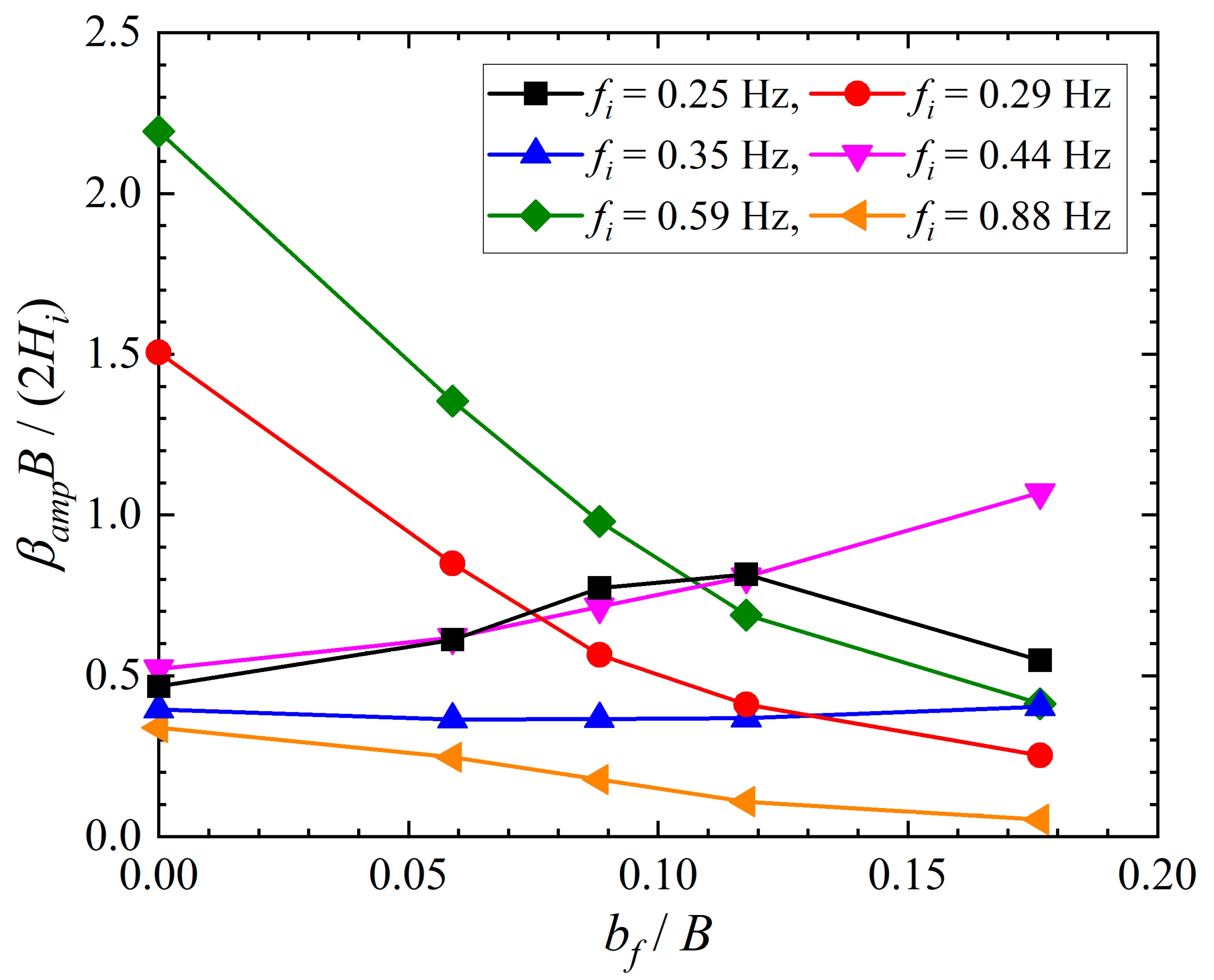
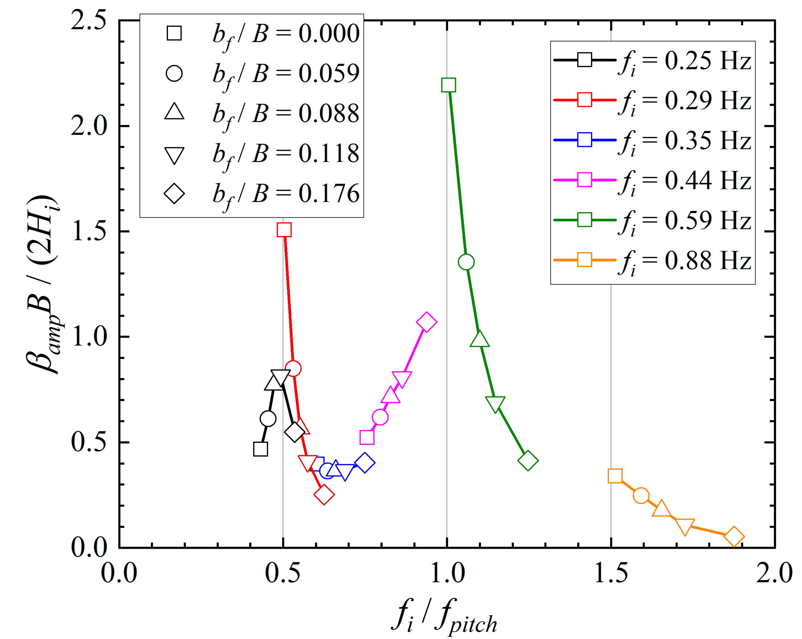
3.3. Total Amplitude of Pitch

Figure 8 shows the relationship between the normalized values of the total amplitude of the pitch β_amp and those of the footing length b_f, where β_amp is the three-period average of the difference between the maximum and minimum values of the pitch. Similar to the heave, the change in β_ampB/(2H_i) with the relative footing length b_f/B is dependent on the incident wave frequency f_i. Specifically, the cases of f_i = 0.29, 0.59, and 0.88 Hz (red, green, and orange lines) show that the value of β_ampB/(2H_i) decreases with an increase in b_f/B. By contrast, for f_i = 0.44 Hz (pink line), β_ampB/(2H_i) increases with b_f / B. This indicates that the value of β_ampB/(2H_i) for f_i = 0.44 Hz has a different trend from f_i = 0.29, 0.59, and 0.88 Hz. For f_i = 0.25 Hz (black line), although β_ampB/(2H_i) increases with b_f/B from b_f/B = 0.000 to 0.118, β_ampB/(2H_i) decreases above b_f/B = 0.118. For f_i = 0.35 Hz (blue line), the change in β_ampB/(2H_i) by b_f/B is not significant.

Figure 9 shows the relationship between the normalized values of the total amplitude of the pitch β_amp and those of the natural frequency of the pitch f_pitch, where the values of f_pitch are shown in Figure 5. For f_i = 0.59 Hz (green line), an increase in the normalized footing length b_f/B decreases the natural frequency f_pitch, giving higher values of f_i/f_pitch departing from 1.0, and this results in a decrease of β_ampB/(2H_i). Conversely, for f_i = 0.44 Hz (pink line), the increase in the normalized footing length b_f/B also results in higher values of f_i/f_pitch, which comes closer to 1.0, and thus the values of β_ampB/(2H_i) are amplified. A similar tendency can be observed for f_i = 0.29 Hz (red line) and 0.25 Hz (black line) around f_i/f_pitch = 0.5. Table 3 indicates that the values of the Goda’s nonlinear parameter Π for f_i = 0.25 and 0.29 Hz exceed 0.1, which is outside the applicable range of the small-amplitude wave theory [12]. This suggests that the incident waves for f_i = 0.25 and 0.29 Hz can contain high frequency components, such as 2f_i; hence, β_ampB/(2H_i) is considered to have increased even when f_i/f_pitch is approximately 0.5, as described above. For this reason, the total amplitude of the pitch β_amp would be reduced by designing caissons, such that the condition of f_i/f_pitch ≈ 0.5 and 1.0 is avoided adjusting the footing length b_f.

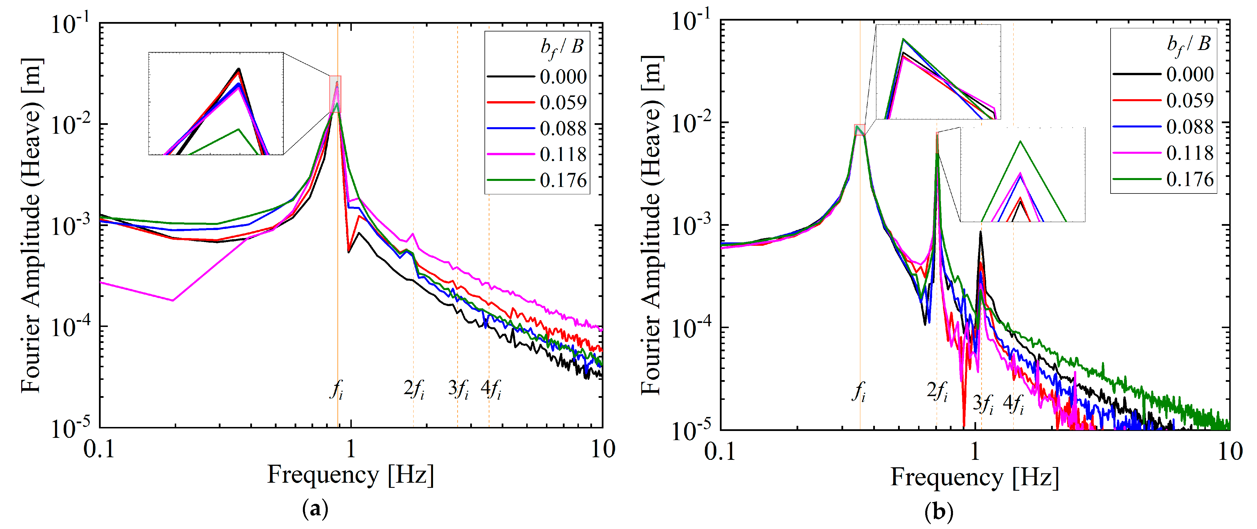
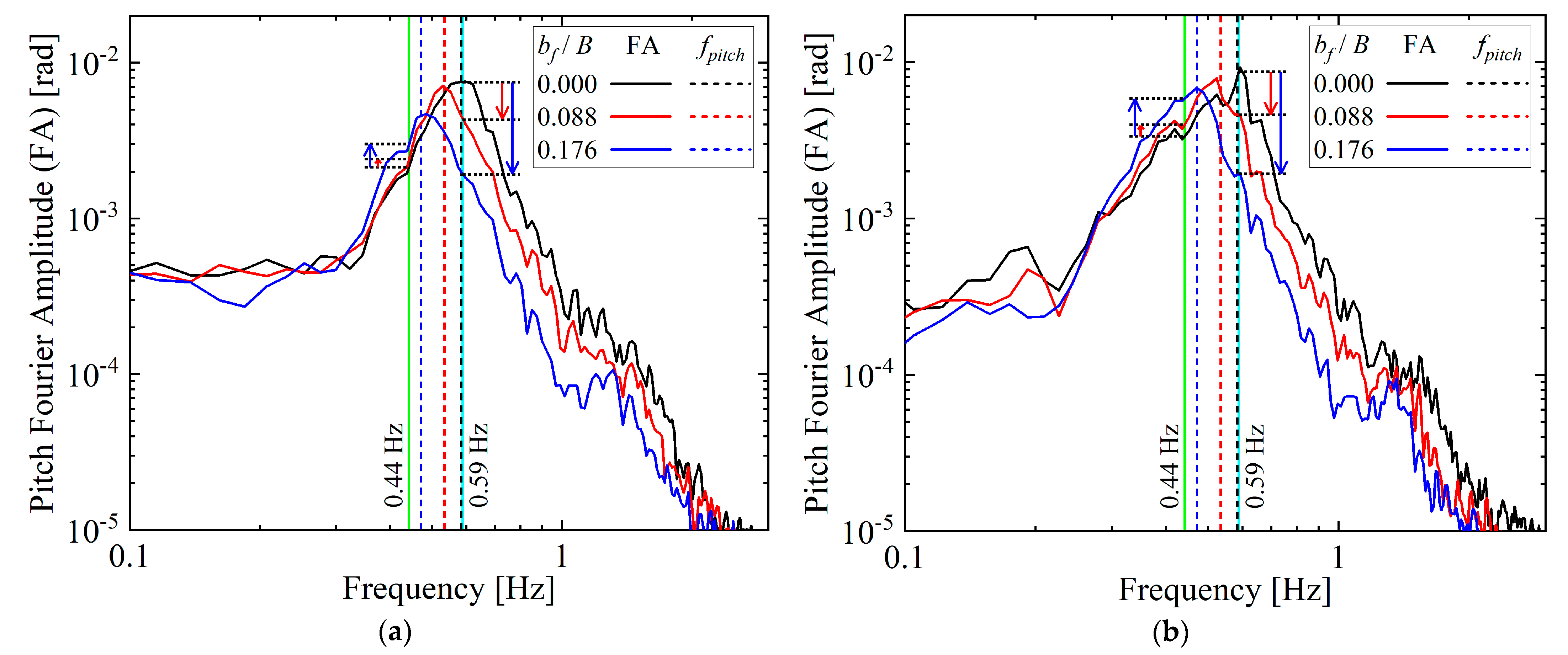
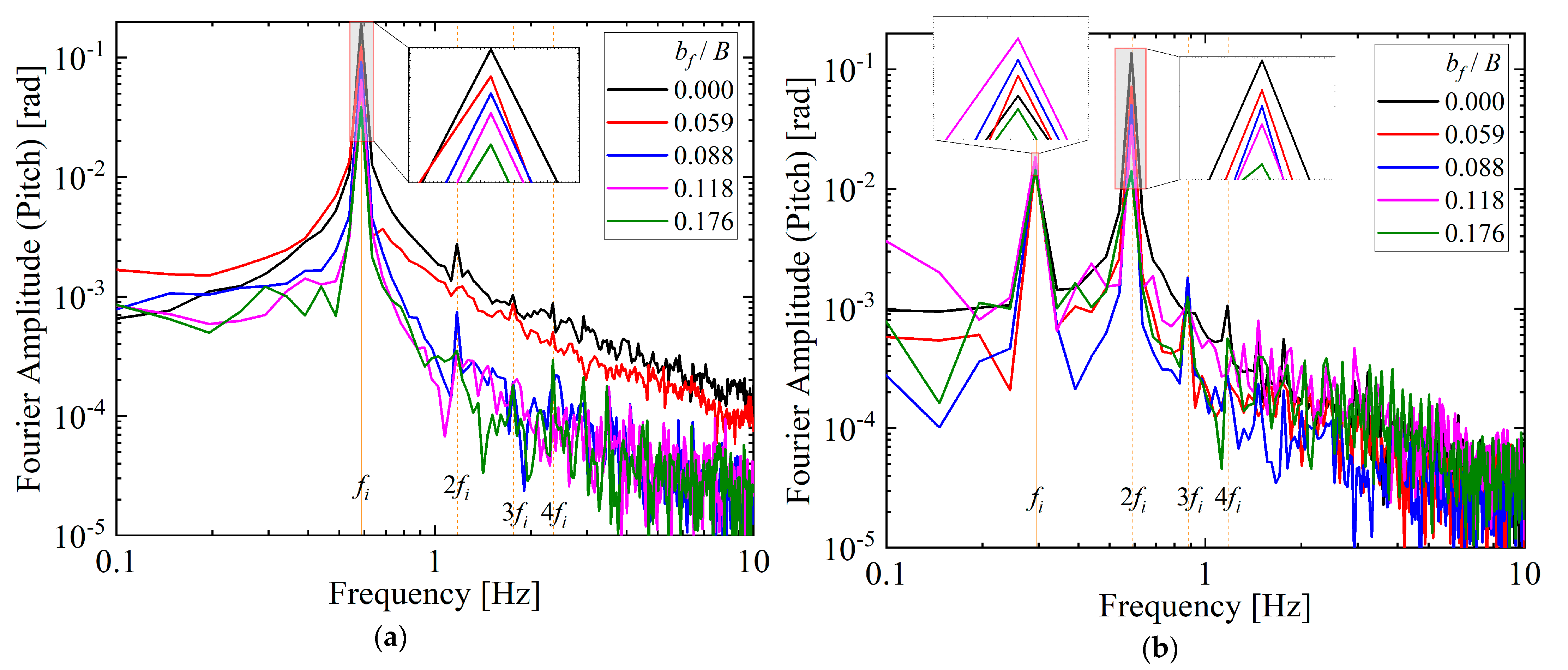
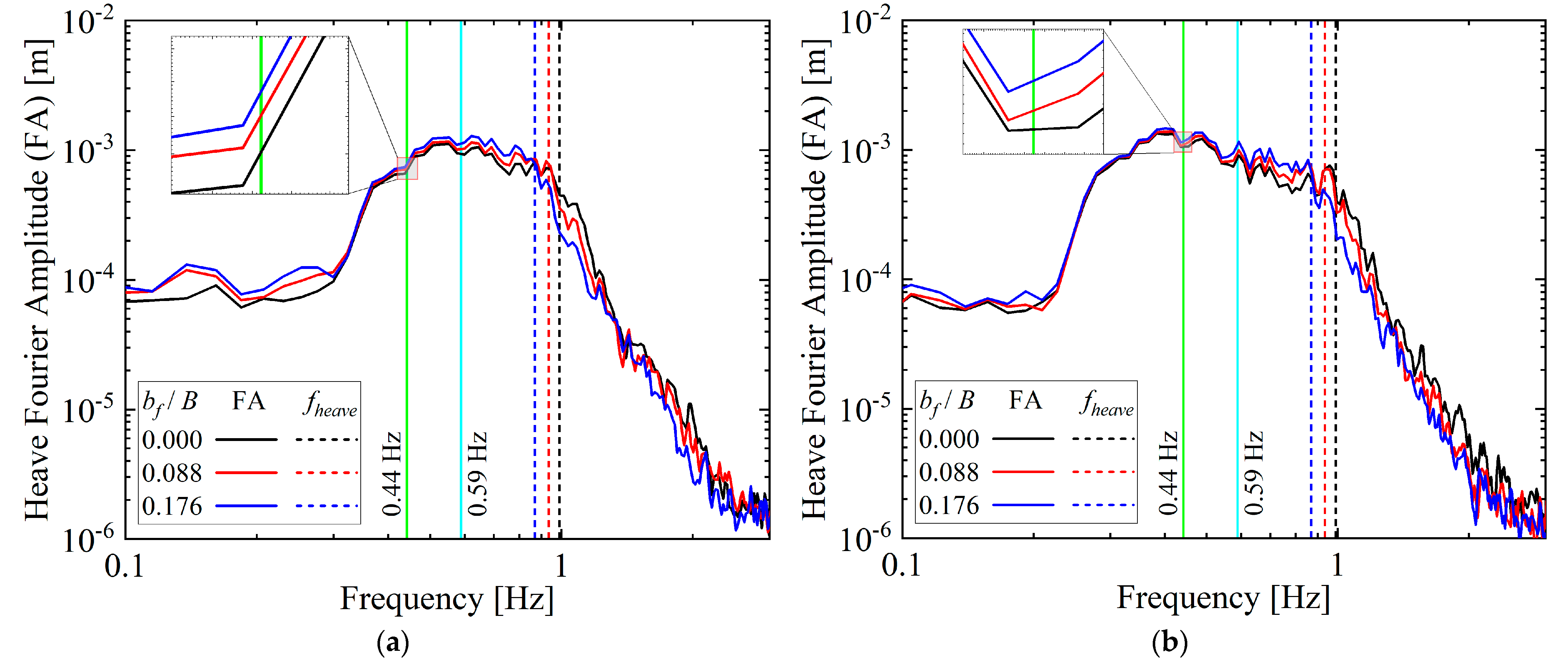
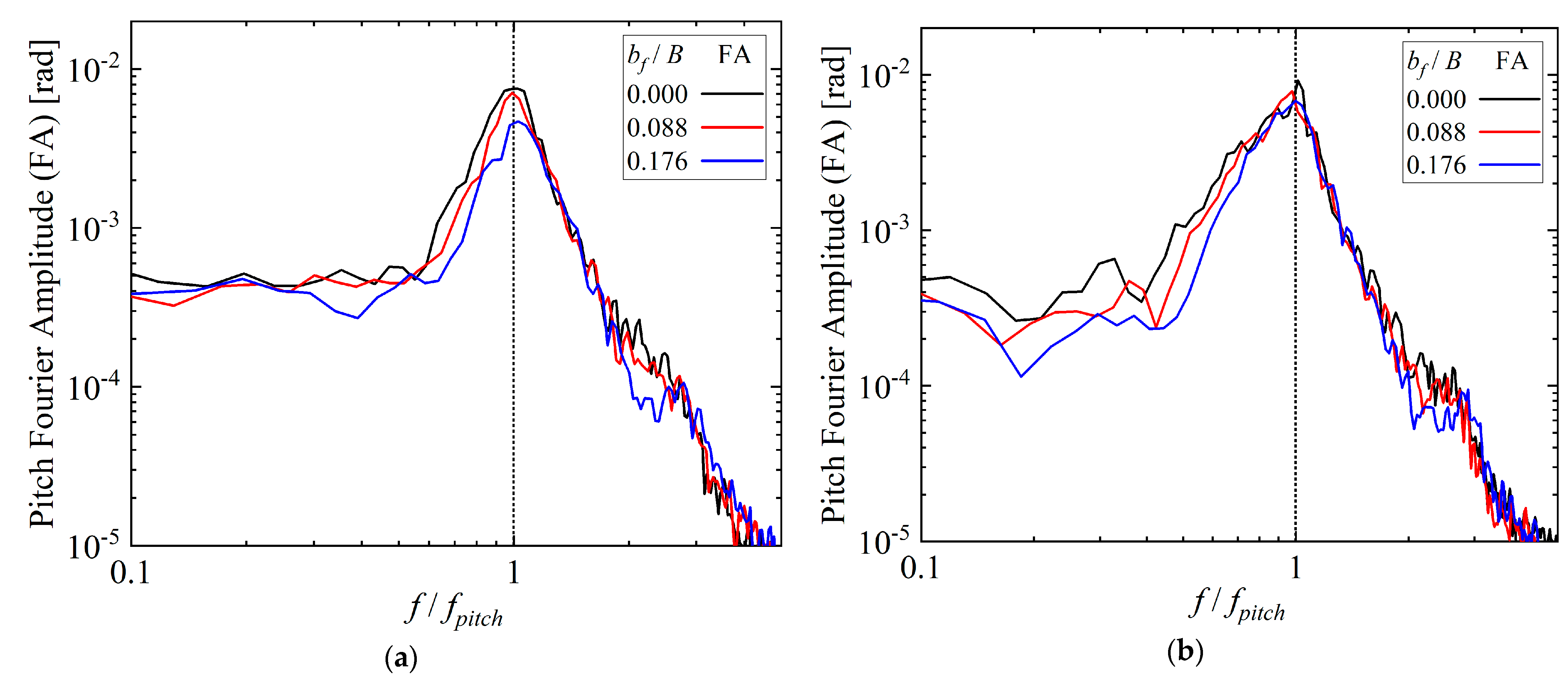
3.4. Fourier Amplitude of Heave and Pitch

Figure 10 and Figure 11 show the Fourier amplitudes of the heave and pitch, where the Fourier amplitudes are calculated using the Python SciPy library. In the figure, the orange solid line represents the incident wave frequency f_i, and the orange dotted lines represent 2f_i, 3f_i, and 4f_i.

From Figure 10a and Figure 11a, the peak of the Fourier amplitude can be observed around f_i. Furthermore, the values of this peak decrease with an increase in the relative footing length b_f/B. This trend corresponds to ζ_amp/H_i and β_ampB/(2H_i), which decrease with an increase in b_f/B, as shown in Figure 6 and Figure 8.

From Figure 10b and Figure 11b, the peak of the Fourier amplitude can be observed not only around f_i, but also around 2f_i and 3f_i. In the cases shown in Figure 10b, the peak values around f_i and 2f_i are comparable. Furthermore, although the peak values around f_i are not significantly affected by b_f/B, the peak values around 2f_i increase with b_f/B. In the cases shown in Figure 11b, the peak values around 2f_i are larger than those around f_i. Furthermore, the peak values around 2f_i decrease with an increase in b_f/B, which is the same trend as ζ_amp/H_i shown in Figure 6 and β_ampB/(2H_i) shown in Figure 8.

From these results, it is revealed that the change in ζ_amp/H_i and β_ampB/(2H_i) with b_f/B can be explained on the basis of the components of the Fourier amplitude around f_i and 2f_i. For high-frequency incident waves (i.e., short-period incident waves), the high-frequency components above 2f_i are not significant, and ζ_amp/H_i and β_ampB/(2H_i) are dominated by the components around f_i. For low-frequency incident waves (i.e., long-period incident waves), the peak around 2f_i is the main component, and ζ_amp/H_i and β_ampB/(2H_i) are dominated by the components around 2f_i.

4. Numerical Conditions

The three-dimensional coupled fluid–structure–sediment–seabed interaction model (FS3M) [5] was used in the hydraulic model experiments.

FS3M consists of a main solver and four modules. The main solver is a large-eddy simulation (LES) model for an incompressible viscous air–water two-phase flow that considers the motion of movable objects. The first module is a volume-of-fluid (VOF) module that tracks the air–water interface motion. The second module is an immersed-boundary (IB) module based on the body-force type of the IB method for fluid–structure interaction (FSI) analysis of movable objects. The third module is a sediment-transport (ST) module that computes the profile evolution of a sediment bed induced by bedload and suspended sediment transport, and suspended sediment concentration that considers all transport processes. The fourth module is a finite element model (FEM) module for coupled soil–water analysis of the sediment bed. The VOF, IB, and ST modules are connected to the main solver through a two-way coupling procedure implemented at every time step to ensure fluid–structure–sediment interaction. In this study, the main solver and the VOF and IB modules were employed to compute the wave–caisson interaction.

A region of limited extent around the caisson was modeled to reduce the computational cost. Specifically, the length of the region in the wave direction was limited to 3.0 m for regular waves and 6.0 m for irregular waves. Figure 12 shows the schematic of the computational domain. As shown in the figure, artificial damping zones with a length of 14.0 m, more than twice the longest incident wavelength analytically calculated using the dispersion relationship, were set at the offshore and onshore edges of the domain. To reduce the influence of air-phase turbulence, the domain was extended to 1.0 m above the still water surface. The caisson with the same specifications as that in the hydraulic model experiments was floated in the domain. The length of the footings b_f was changed to 0.00 (no footing), 0.03, and 0.06 m. The density of the PVC of the caisson and footings was set at 1.41 × 10³ kg/m³, and the density of the weights in the caisson was set at 7.84 × 10³ kg/m³.

The region where the caisson could move around the still water level was divided into 2.5 × 5.0 × 5.0-mm uniform cells. The remainder of the domain was divided into non-uniform cells with an increasing size in all directions to further reduce the computational cost. Figure 13 shows the numerical cells around the initial position of the caisson. In the figure, the water surface is shown in light blue, the caisson in yellow green, and the weights in gray inside the caisson. The offshore and onshore boundaries were set according to the Sommerfeld radiation condition to reduce the reflected waves. The slip condition was applied to the bottom, forward, and backward boundaries, and a constant-pressure condition was applied to the top boundary. The gravitational acceleration was set at 9.81 m/s², the density of water at 9.97 × 10² kg/m³, the density of air at 1.18 kg/m³, the kinematic viscosity of water at 8.93 × 10⁻⁷ m²/s, the kinematic viscosity of air at 1.54 × 10⁻⁵ m²/s, and the surface tension coefficient at 7.20 × 10⁻² N/m.

Similar to that in the hydraulic model experiments, free and forced oscillation simulations were conducted. In the free oscillation simulations, the natural frequency of the heave f_heave was computed by providing the caisson with an initial vertical velocity. The natural frequency of the pitch f_pitch was computed by providing the caisson with an initial angular velocity around the pitch axis. In the forced oscillation simulations, regular and irregular waves were generated toward the floating caisson. For the regular waves, the same wave conditions were used in the hydraulic model experiments. Specifically, the incident wave height H_i was set at 0.03 m, and the incident wave period T_i was changed to 1.13, 1.70, 2.26, 2.83, 3.39, and 3.96 s. The computations were performed up to 32.0 s that corresponded to approximately eight waves for T_i = 3.96 s. For the irregular waves, the modified Bretschneider–Mitsuyasu spectrum with a significant wave height of H_s = 0.03 m and a significant wave period of T_s = 1.70 and 2.26 s (i.e., significant wave frequency f_s = 0.59 and 0.44 Hz) was used. The irregular waves were structured as a superposition of 500 sinusoidal waves with a frequency of 0.5f_s to 5.0f_s. The computations were performed up to 187.0 s for T_s = 1.70 s and 248.6 s for T_s = 2.26 s, to compute more than 100 waves. This is because more than 100 waves must be computed to avoid bias in the occurrence frequency of the wave height for irregular waves [13]. For T_s = 2.26 s, the computations took 99.7 days using a workstation with Intel Xeon E5-2687W (Intel Corp., CA, USA, 3.10 GHz) and 32 GB memory.

5. Numerical Results and Discussion

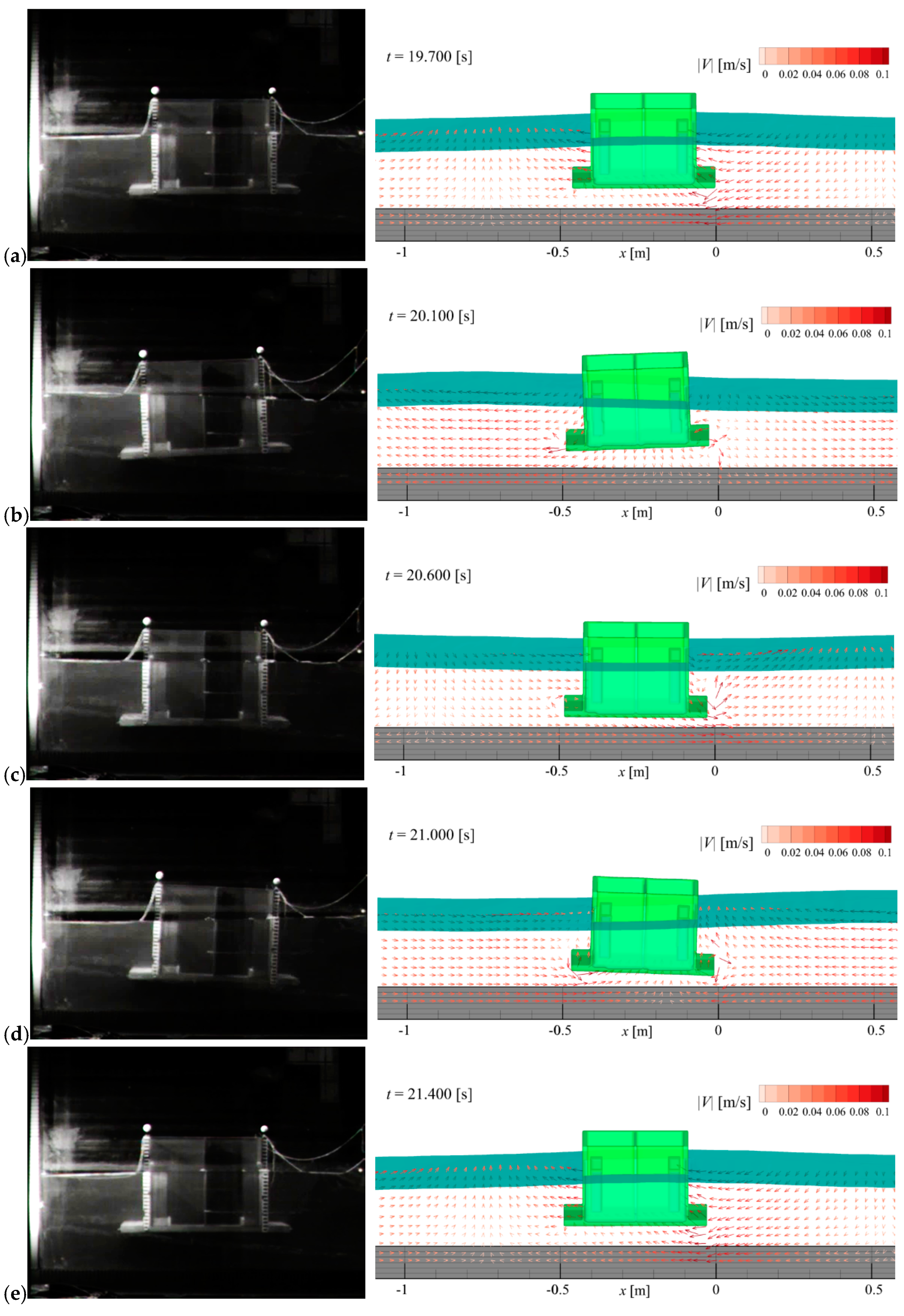
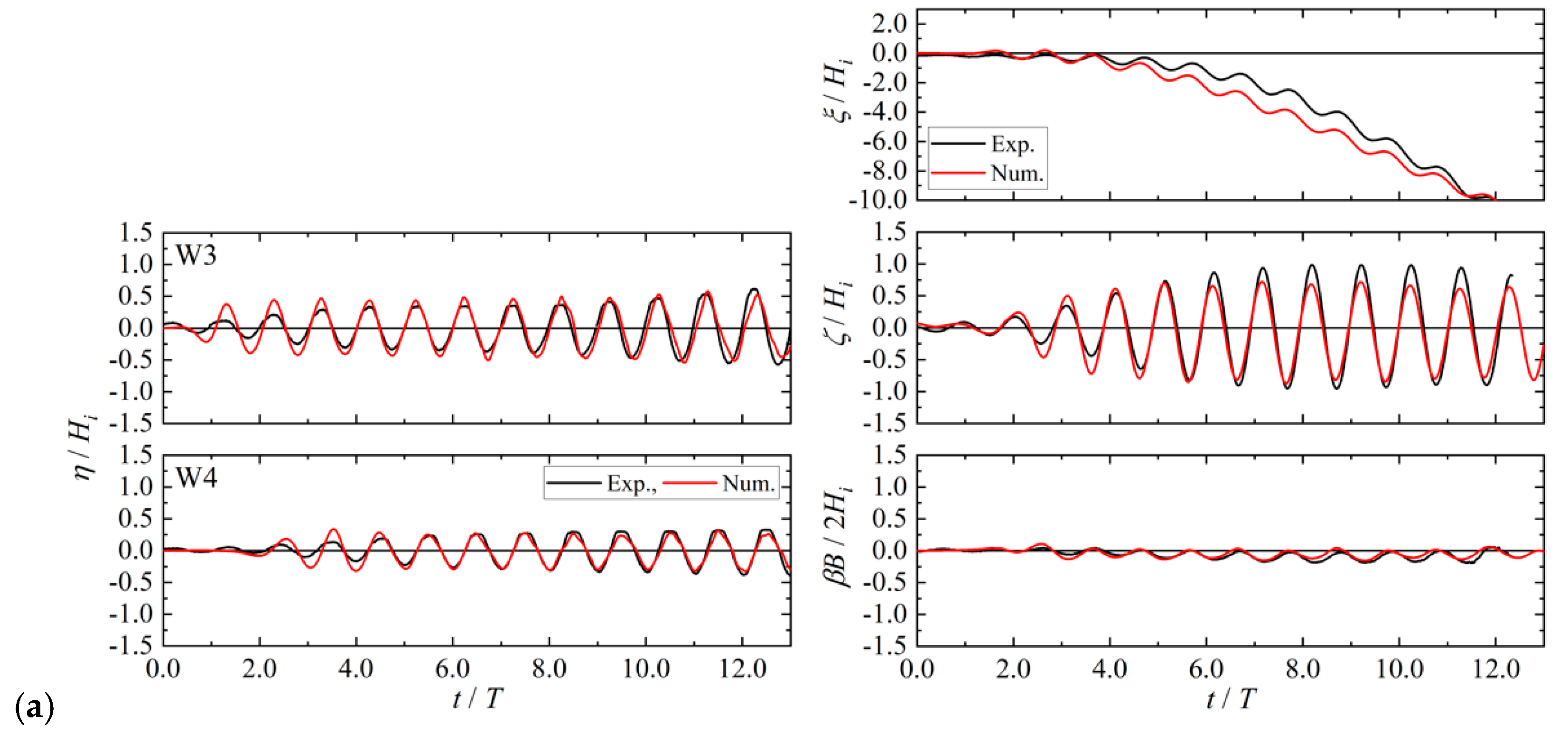
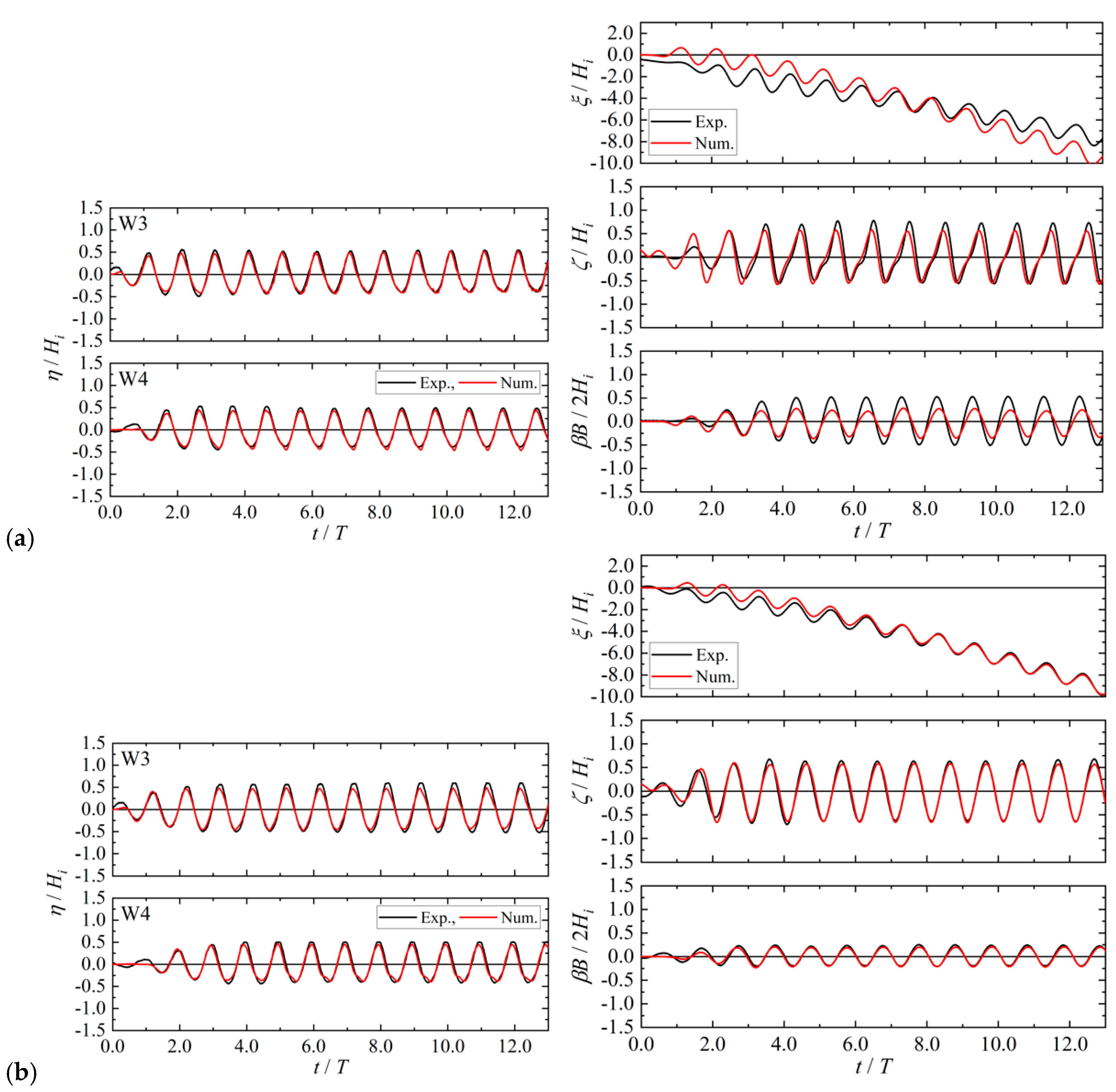
5.1. Comparison under Regular Waves Based on Hydraulic Model Experiments

Figure 14 shows a comparison of the natural frequencies of the heave f_heave and pitch f_pitch, where the experimental data are the same as those in Figure 5.

As shown in Figure 14, the value of f_pitch for b_f = 0 mm is slightly overestimated, and the value of f_heave for b_f = 60 mm is slightly underestimated. However, the numerical results and the experimental data are in very good agreement.

Cross-sectional two-dimensional (2-D) computations with a low computational cost were performed as preliminary computations. Although no figure is presented here, from the numerical results, we found that the values of f_heave and f_pitch were underestimated. In the 2-D computations, the water mass under the caisson can only move to and out from the offshore and onshore sides of the caisson; hence, it took more time for the caisson to move. This suggests that it is essential to conduct three-dimensional computations despite the high computational cost, when dealing with the motion of floating bodies.

Figure 15 shows a comparison of wave deformation around the caisson. The left panel shows snapshots of a movie captured using the high-speed camera in the hydraulic model experiments, and the right panel shows snapshots of the numerical results obtained through the numerical simulations. In the right panel, the water surface is shown in light blue, the caisson in yellow green, and the weights in gray inside the caisson. The flow velocity at the central cross section (y = 0) in the water phase is represented by vectors, and |V| is the magnitude of the vectors. The variable t is the time. The animation corresponding to the right panel of Figure 15 is shown in Video S1.

As shown in Figure 15a, the caisson is almost horizontal when the wave crest with landward (leftward) flow velocity passes through the caisson. After the wave crest passes, the caisson leans toward the onshore area (Figure 15b). At the passage of the wave trough with seaward (rightward) flow velocity, the caisson is almost horizontal again (Figure 15c). Thereafter, the caisson leans toward the offshore area (Figure 15d). In Figure 15e, one wave period after Figure 15a, the caisson returns to an almost horizontal position. The same process can be observed from the experimental data (left panel) and numerical results (right panel).

Figure 16, Figure 17 and Figure 18 show a comparison of the water surface fluctuations η at W3 and W4 (see Figure 1 and Figure 12) and the surge ξ, heave ζ, and pitch β of the caisson. In the figures, the black lines represent the experimental data, and the red lines represent the numerical results. The variable t in the horizontal axis represents the time.

Overall, the drift in the surge direction is overestimated. One of the reasons for this is that large motion of the caisson in the surge direction was constrained by the mooring lines in the hydraulic model experiments, while the caisson was free-floating without mooring in the numerical simulations.

The experimental value of the natural frequency of the heave was f_heave = 0.94 Hz for b_f = 30 mm (see Figure 5). When the incident wave frequency f_i is close to f_heave (Figure 17a, f_i = 0.88 Hz), the amplitude of the heave ζ is underestimated. Similarly, the experimental values of the natural frequency of the pitch were f_pitch = 0.59 Hz for b_f = 0 mm and f_pitch = 0.47 Hz for b_f = 60 mm. When f_i is close to f_pitch, Figure 16a (f_i = 0.59 Hz) and Figure 18a (f_i = 0.44 Hz) show that the amplitude of pitch β is underestimated. Although all the figures are not presented here, we can observe that when f_i is close to f_heave or f_pitch, the corresponding motion, ξ or β, is underestimated. From the characteristics of the IB method employed in FS3M, energy is additionally consumed to drive the fluid inside the volume excluded by the caisson [14]; hence, this influence is considered to be noticeable, particularly during resonance.

For low-frequency waves, Figure 16b (f_i = 0.35 Hz) and Figure 17b (f_i = 0.29 Hz) show that the waveform of the troughs of the water surface elevation η and heave ζ is slightly different. In these cases, as mentioned in Section 3.3, incident waves can contain high-frequency components. Furthermore, the magnitude of the high-frequency components can be different because of the different wave generation methods, that is, the piston-type wave generator in the hydraulic experiments and the wave generation source/sink in the numerical simulations. This leads to slightly different characteristics, phase, and shape of the waves observed at the wave gauge locations.

Except for the points above, the numerical results are in good agreement with the experimental data.

Using these results, we can demonstrate the predictive capability of FS3M, both qualitatively and quantitatively.

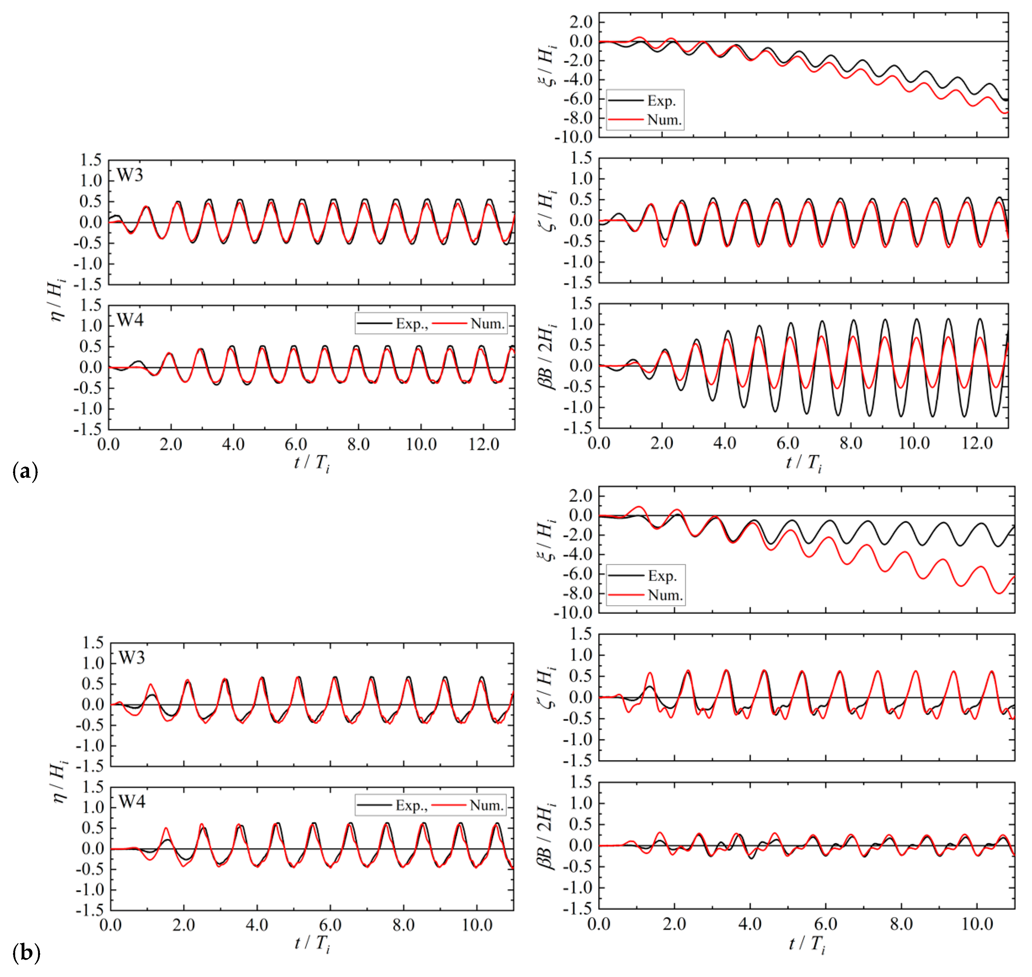
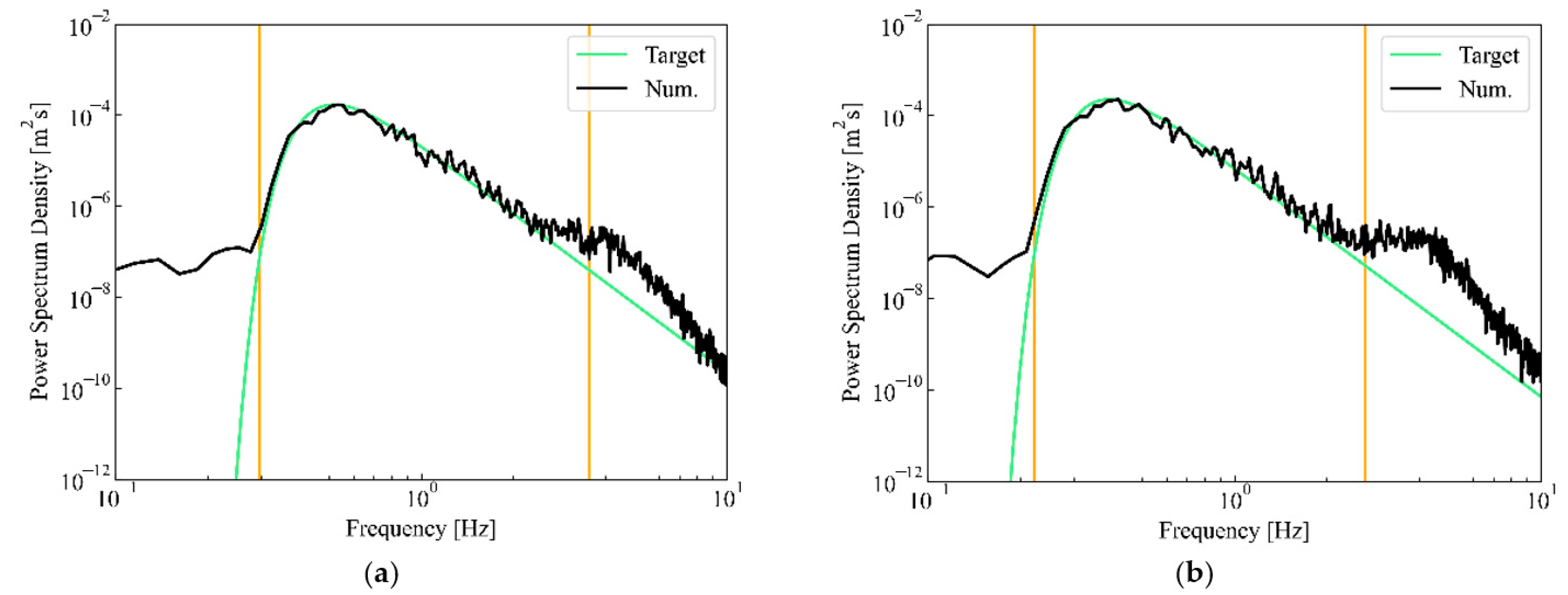
5.2. Response of Caisson under Irregular Waves

Figure 19 shows the power spectrum density calculated from the water surface fluctuations at x = 0 and y = 0 in the absence of the caisson. In the figure, the yellow green line represents the target modified Bretschneider–Mitsuyasu spectrum, and the orange lines represent the lower and upper limits of the components constituting the irregular waves, i.e., 0.5f_s and 5.0f_s. Although the target spectrum (green line) is slightly overestimated near the upper limit of 5.0f_s (right orange line), the irregular waves with the target spectrum can be generated accurately in the range of 0.5f_s to 5.0f_s.

Figure 20 shows the Fourier amplitude of the heave. In the figure, the green and light blue lines represent 0.44 and 0.59 Hz, which are the same as the incident wave frequencies f_i used for the regular waves.

In Section 3.4, we conclude that the change in ζ_amp/H_i with b_f/B can be explained on the basis of the Fourier amplitude. In Section 3.2, Figure 5 shows that the value of ζ_amp/H_i increased with b_f/B for 0.44 and 0.59 Hz. Correspondingly, Figure 20 shows that the Fourier amplitudes at 0.44 (green line) and 0.59 Hz (light blue line) increase with an increase in b_f/B. This suggests that the Fourier amplitude of each frequency component corresponds to the results obtained for the regular waves.

Furthermore, the relationship between the Fourier amplitude and b_f/B is reversed below and above 0.9–1.0 Hz, which is close to the natural frequency of the heave f_heave. For a lower frequency than 0.9–1.0 Hz, as mentioned above, the Fourier amplitude increases with b_f/B. By contrast, for a higher frequency than 0.9–1.0 Hz, the Fourier amplitude decreases with an increase in b_f/B. This suggests that the footing has the effect of amplifying the low-frequency components below the natural frequency f_heave and reducing the high-frequency components above the natural frequency f_heave. This effect is enhanced with the increase in the footing length b_f.

Figure 21 shows the Fourier amplitude of the pitch. In the figure, the yellow green and light blue lines represent 0.44 and 0.59 Hz, respectively.

Similar to the case of ζ_amp/H_i, Section 3.4 reveals that the change in β_ampB/(2H_i) with b_f/B can be explained by the Fourier amplitude. In Section 3.2, based on Figure 7, it is understood that as the value of b_f/B increases, the value of β_ampB/(2H_i) also increases at 0.44 Hz and decreases at 0.59 Hz. Correspondingly, as indicated using the upward and downward arrows in Figure 21, the Fourier amplitude increases at 0.44 Hz and decreases at 0.59 Hz with an increase in b_f/B. Similar to the case of the heave, the Fourier amplitude of each frequency component corresponds to the results of the regular waves.

As the value of b_f/B increases, the peak of the Fourier amplitude moves to the low-frequency side with the decrease in its value. Similar to that for the heave, the relationship between the Fourier amplitude and b_f/B is reversed below and above 0.5–0.6 Hz, which is close to the natural frequency of the pitch f_pitch. From this result, it is understood that the footing also amplifies the low-frequency components below the natural frequency f_pitch and reduces the high-frequency components above the natural frequency f_pitch. Furthermore, this effect is enhanced with an increase in the footing length b_f, particularly for reducing the high-frequency components.

Figure 22 shows the normalized form of the horizontal axis of Figure 21 using the natural frequency f_pitch, where f is the frequency.

From Figure 22, the peak of the Fourier amplitude can be observed around f/f_pitch = 1 regardless of the incident wave frequency f_i. This suggests that the Fourier amplitude is strongly affected by the natural frequency f_pitch changing with b_f/B.

Figure 23 shows the normalized significant values of the total amplitude of the heave ζ_amps and the total amplitude of the pitch β_amps. The values of ζ_amps and β_amps were calculated using the same procedure as that of the significant wave height.

As shown in Figure 20, the relationship between the Fourier amplitude of the heave and b_f / B was reversed below and above 0.9–1.0 Hz. The significant wave frequencies f_s (=0.44 and 0.59 Hz) used here are all smaller than 0.9 to 1.0 Hz; hence, Figure 21 indicates that ζ_amps/H_s tends to increase with b_f/B.

Furthermore, Figure 21 shows that the relationship between the Fourier amplitude of the pitch and b_f/B is reversed below and above 0.5–0.6 Hz and the higher frequency components are significantly reduced with an increase in b_f/B. From a comparison between Figure 7 and Figure 23, for f_i = f_s = 0.59 Hz, the same trend can be observed between the regular and irregular waves. By contrast, for f_i = f_s = 0.44 Hz, the trend is different between the regular and irregular waves. This is because the values of β_ampsB/(2H_i) are more strongly affected by the significant decrease in the higher frequency components, even if f_s = 0.44 Hz is smaller than 0.5–0.6 Hz. This suggests that it is essential to examine the motion of a caisson under irregular waves when assessing the effect of footings in an actual marine environment.

6. Conclusions

In this study, the motion of a floating caisson with footings was investigated through hydraulic model experiments and numerical simulations using FS3M. The main conclusions of this study are as follows:

• Regarding the heave of the caisson, the natural frequency of the heave f_heave was little affected by the footing length b_f. This suggests that it is essential to design caissons such that the natural frequency of the heave f_heave does not coincide with the frequency of waves, as expected using towing operations.
• Regarding the pitch of the caisson, the relative total amplitude of the pitch β_ampB/(2H_i) increased as the relative incident wave frequency f_i/f_pitch approached 0.5 and 1.0. This suggests that the total amplitude of the pitch β_amp could be reduced by designing caissons with the footing length b_f, such that the condition of f_i/f_pitch ≈ 0.5 and 1.0 is avoided.
• From a comparison with the experimental data, the predictive capability of the FS3M was demonstrated in terms of the water surface fluctuations and the motion of the caisson, except under the condition of resonance.
• The Fourier amplitudes of the heave and pitch under irregular waves showed that the footings exhibited an amplification of their low-frequency components and a reduction in their high-frequency components, and this effect was enhanced by increasing the footing length b_f.
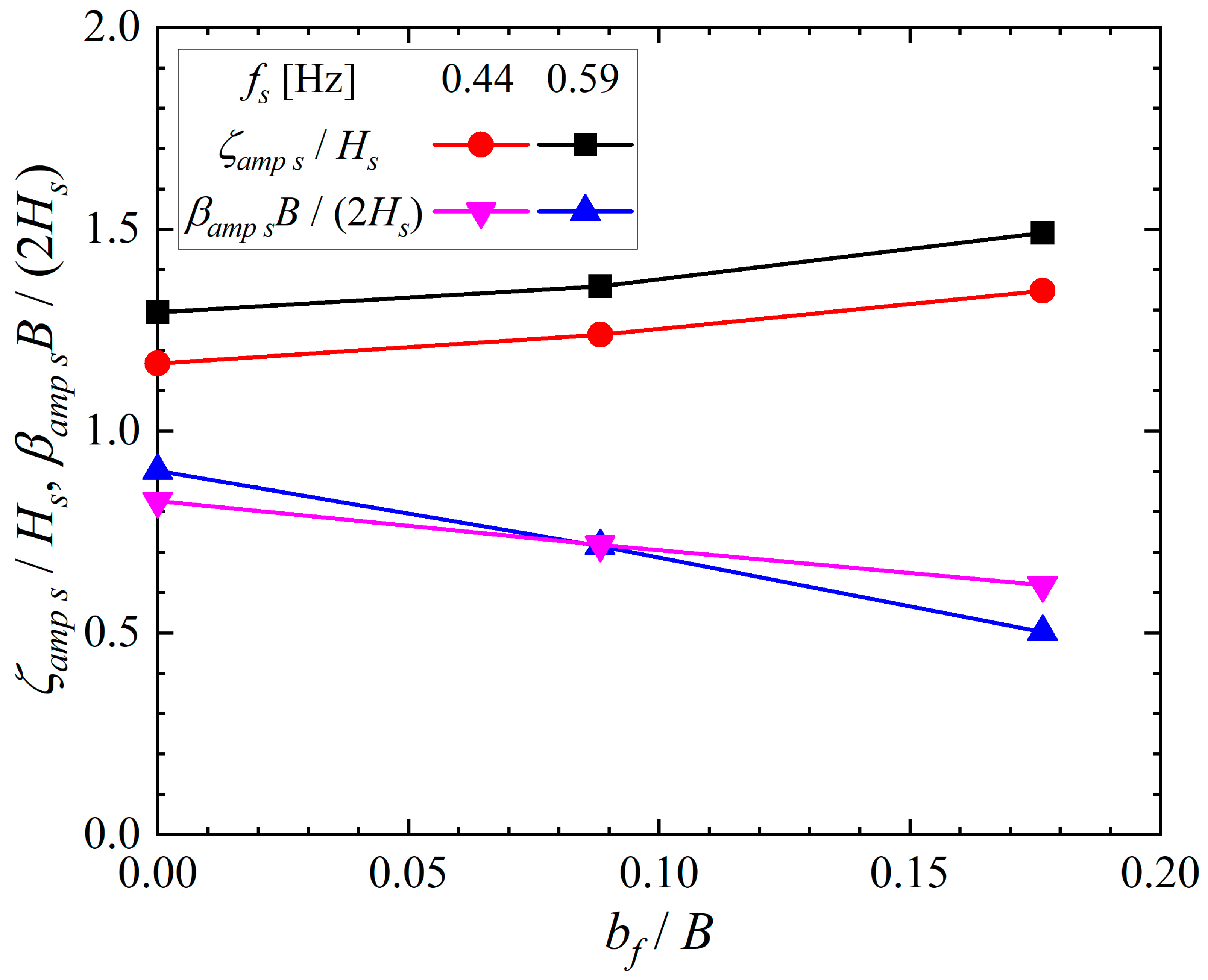
• The significant total amplitudes of the heave ζ_amps and pitch β_amps under irregular waves indicated a different trend from that of the regular waves. This suggests that it is essential to examine the motion of a caisson under irregular waves when evaluating the effect of footings in an actual marine environment.

The response of the caisson, however, was clarified unsatisfactorily due to the small-scale experiments and simulations where scale effects were unavoidable. Furthermore, the effect of the footings was not examined under lower- and higher-frequency components of waves. The motions of the caisson other than the surge, heave, and pitch were not discussed due to the lack of experimental data. To address these issues, it is recommended that further studies be conducted under the six DOF motion in a larger scale.

References

1. Chakrabarti, S.K.; Chakrabarti, P.; Krishna, M.S. Design, construction, and installation of a floating caisson used as a bridge pier. J. Waterway Port Coastal and Ocean Eng. 2006, 132, 143–156. [Google Scholar] [CrossRef]
2. Huang, Z.; Liu, C.; Kurniawan, A.; Tan, S.K.; Nah, E. Responses of a floating rectangular caisson to regular waves: A comparison of measurements with time-domain and frequency-domain simulations. In Proceedings of the Asian and Pacific Coasts 2009, Singapore, 13–16 October 2009. [Google Scholar]
3. Huang, X.; Zhang, W.; Jiang, B.; Lv, Y. Experimental study on the offshore positioning and installing of large caisson. Appl. Mech. Mater. 2014, 580–583, 2129–2133. [Google Scholar] [CrossRef]
4. Kotake, Y.; Oomukai, Y.; Matsumura, A.; Nakamura, T. A study on the behaviour of a relatively small caisson floating in wave fields and its effective installation method. In Proceedings of the Coasts, Marine Structures and Breakwaters Conference: Realising the Potential, Liverpool, UK, 5–7 September 2017. [Google Scholar]
5. Nakamura, T.; Mizutani, N. Development of fluid-sediment-seabed interaction model and its application. In Proceedings of the 34th International Conference on Coastal Engineering, Seoul, Korea, 15–20 September 2014. [Google Scholar]
6. Meneses, L.; Sarmiento, J.; de los Dolores, D.; Blanco, D.; Guanche, R.; Losada, I.J.; Rodriguez de Segovia, M.F.; Ruiz, M.J.; Martín, M.A.; Conde, M.J.; et al. Large scale physical modelling for a floating concrete caisson in marine works. In Proceedings of the ASME 2018 37th International Conference on Ocean, Offshore and Arctic Engineering, Madrid, Spain, 17–22 June 2018. [Google Scholar]
7. Gu, H.; Wang, H.; Zhai, Q.; Feng, W.; Cao, J. Study on the dynamic responses of a large caisson during wet-towing transportation. Water 2021, 13, 126. [Google Scholar] [CrossRef]
8. Nagasawa, D.; Miyasaka, M.; Wada, Y.; Ikegami, K. Development of motion estimation technique for caisson-type structure considering nonlinear damping force. Proc. Coast. Eng. JSCE 1997, 44, 821–825. (In Japanese) [Google Scholar]
9. Ishimi, G.; Shiraishi, S.; Nazato, K. Characteristics of Motions of a Caisson for Breakwater during Installation and Limit Condition of Works at Ocean-Facing Ports; Technical Note of the Port and Harbour Research Institute, Ministry of Transport: Yokosuka, Japan, 1996; (In Japanese with English Abstract). [Google Scholar]
10. Michimae, T.; Sanuki, H.; Imamura, T.; Sakai, K.; Koga, D.; Niwa, T.; Itou, Y. Seakeeping properties of towing a massive and asymmetric caisson. J. Jpn. Soc. Civil Eng. Ser. B2 (Coastal Eng.) 2018, 74, I_1051–I_1056, (In Japanese with English abstract). [Google Scholar] [CrossRef]
11. Goda, Y. Random Seas and Design of Maritime Structures, 3rd ed.; Advanced Series of Ocean Engineering Vol. 33; World Scientific Publishing Co.: Singapore, 2010; 418p. [Google Scholar]
12. Iwagaki, Y. Latest Coastal Engineering; Morikita Publishing Co.: Tokyo, Japan, 1987; p. 250. (In Japanese) [Google Scholar]
13. Coastal Development Institute of Technology (CDIT). Practical Computational Examples of CADMAS-SURF; Coastal Development Library No. 30; Coastal Development Institute of Technology: Tokyo, Japan, 2008; p. 364. (In Japanese) [Google Scholar]
14. Suzuki, K.; Inamuro, T. Effect of internal mass in the simulation of a moving body by the immersed boundary method. Comput. Fluid 2011, 49, 173–187. [Google Scholar] [CrossRef]
Figure 1. Wave flume (unit: mm; W3, W4: locations of the wave gauges).
Jmse 09 01129 g001
Figure 2. Caisson (unit: mm): (a) top view; (b) cross-sectional view.
Jmse 09 01129 g002
Figure 3. Definition of the six degree-of-freedom (DOF) motion.
Jmse 09 01129 g003
Figure 4. Initial state of the caisson with the markers and mooring lines.
Jmse 09 01129 g004
Figure 5. Natural frequency of the heave fheave and pitch fpitch of the caisson.
Jmse 09 01129 g005
Figure 6. Relationship between ζamp/Hi and bf/B for the heave motion.
Jmse 09 01129 g006
Figure 7. Relationship between ζamp/Hi and fi/fheave for the heave motion.
Jmse 09 01129 g007
Figure 8. Relationship between βampB/(2Hi) and bf/B for the pitch motion.
Jmse 09 01129 g008
Figure 9. Relationship between βampB/(2Hi) and fi/fpitch for the pitch motion.
Jmse 09 01129 g009
Figure 10. Fourier amplitude of the heave: (a) fi = 0.88 Hz; (b) fi = 0.35 Hz.
Jmse 09 01129 g010
Figure 11. Fourier amplitude of the pitch: (a) fi = 0.59 Hz; (b) fi = 0.29 Hz.
Jmse 09 01129 g011
Figure 12. Computational domain (unit: mm; W3, W4: output locations of water surface fluctuations).
Jmse 09 01129 g012
Figure 13. Numerical cells around the initial position of the caisson.
Jmse 09 01129 g013
Figure 14. Comparison of the natural frequency of the heave fheave and pitch fpitch.
Jmse 09 01129 g014
Figure 15. Comparison of the wave deformation for Ti = 1.70 s (fi = 0.59 Hz) and bf = 60 mm (left: experimental data; right: numerical results): (a) t = 19.7 s, (b) t = 20.1 s, (c) t = 20.6 s, (d) t = 21.0 s, and (e) t = 21.4 s.
Jmse 09 01129 g015
Figure 16. Comparison of the water surface fluctuations η and the surge ξ, heave ζ, and pitch β of the caisson for bf = 0 mm: (a) Ti = 1.70 s (fi = 0.59 Hz); (b) Ti = 2.83 s (fi = 0.35 Hz).
Jmse 09 01129 g016
Figure 17. Comparison of the water surface fluctuations η and the surge ξ, heave ζ, and pitch β of the caisson for bf = 30 mm: (a) Ti = 1.13 s (fi = 0.88 Hz); (b) Ti = 3.39 s (fi = 0.29 Hz).
Jmse 09 01129 g017aJmse 09 01129 g017b
Figure 18. Comparison of the water surface fluctuations η and the surge ξ, heave ζ, and pitch β of the caisson for bf = 60 mm: (a) Ti = 2.26 s (fi = 0.44 Hz); (b) Ti = 1.70 s (fi = 0.59 Hz).
Jmse 09 01129 g018
Figure 19. Power spectrum density of the water surface fluctuations at x = 0 and y = 0 in the absence of the caisson: (a) fs = 0.59 Hz; (b) fs = 0.44 Hz.
Jmse 09 01129 g019
Figure 20. Fourier amplitude (FA) of the heave for the irregular waves: (a) fs = 0.59 Hz; (b) fs = 0.44 Hz.
Jmse 09 01129 g020
Figure 21. Fourier amplitude (FA) of the pitch for the irregular waves: (a) fs = 0.59 Hz; (b) fs = 0.44 Hz.
Jmse 09 01129 g021
Figure 22. Fourier amplitude (FA) of the pitch with the normalized frequency f/fpitch for the irregular waves: (a) fs = 0.59 Hz; (b) fs = 0.44 Hz.
Jmse 09 01129 g022
Figure 23. Significant total amplitude of the heave ζamps and pitch βamps.
Jmse 09 01129 g023