
Ship Motion Planning for MASS Based on a Multi-Objective Optimization HA* Algorithm in Complex Navigation Conditions

Abstract
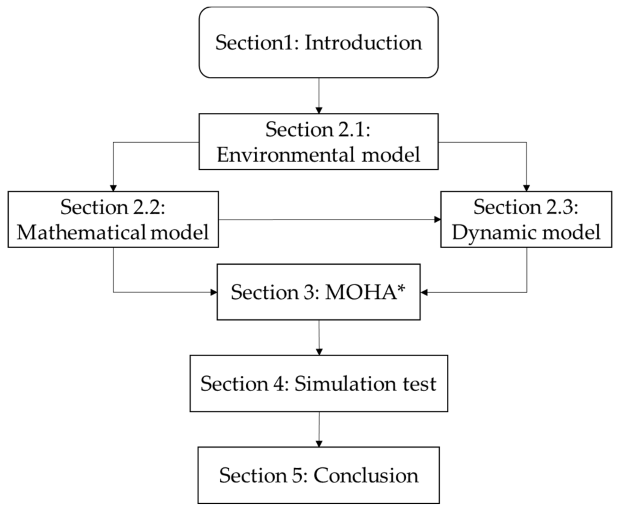
:1. Introduction
2. Materials and Methods
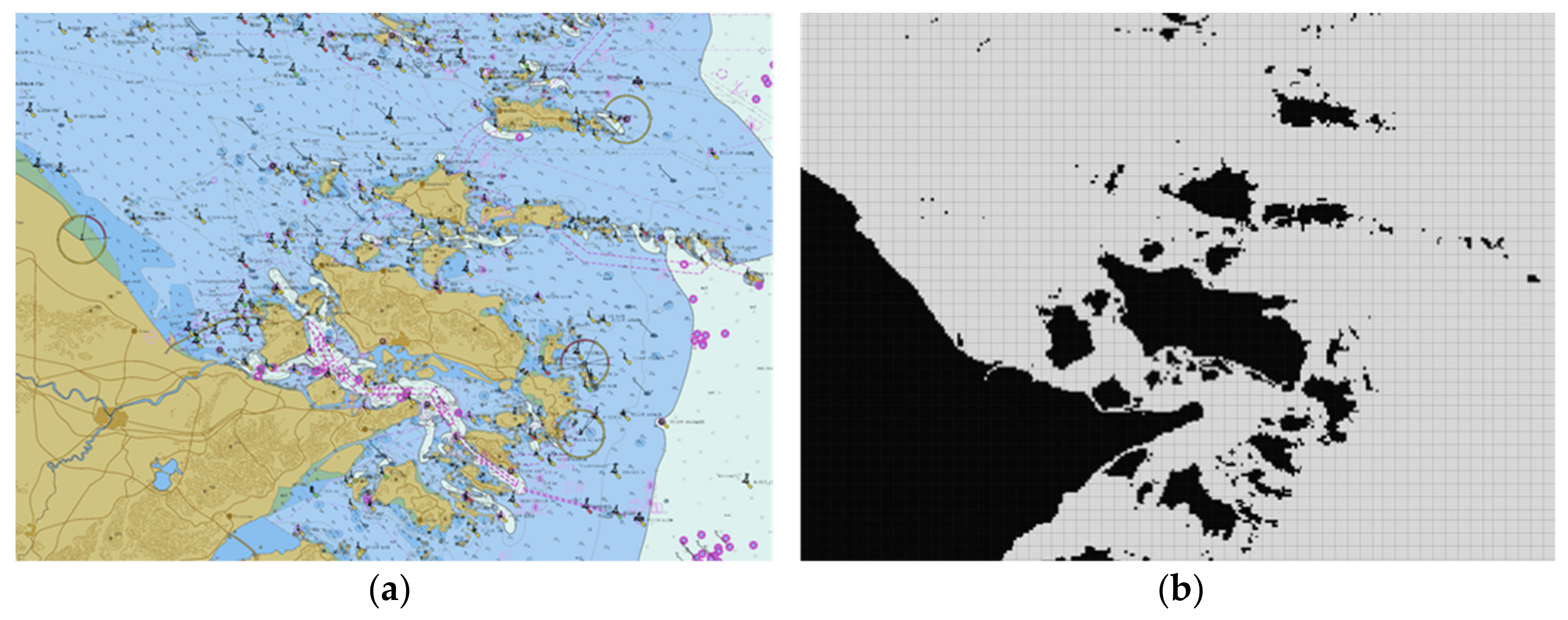
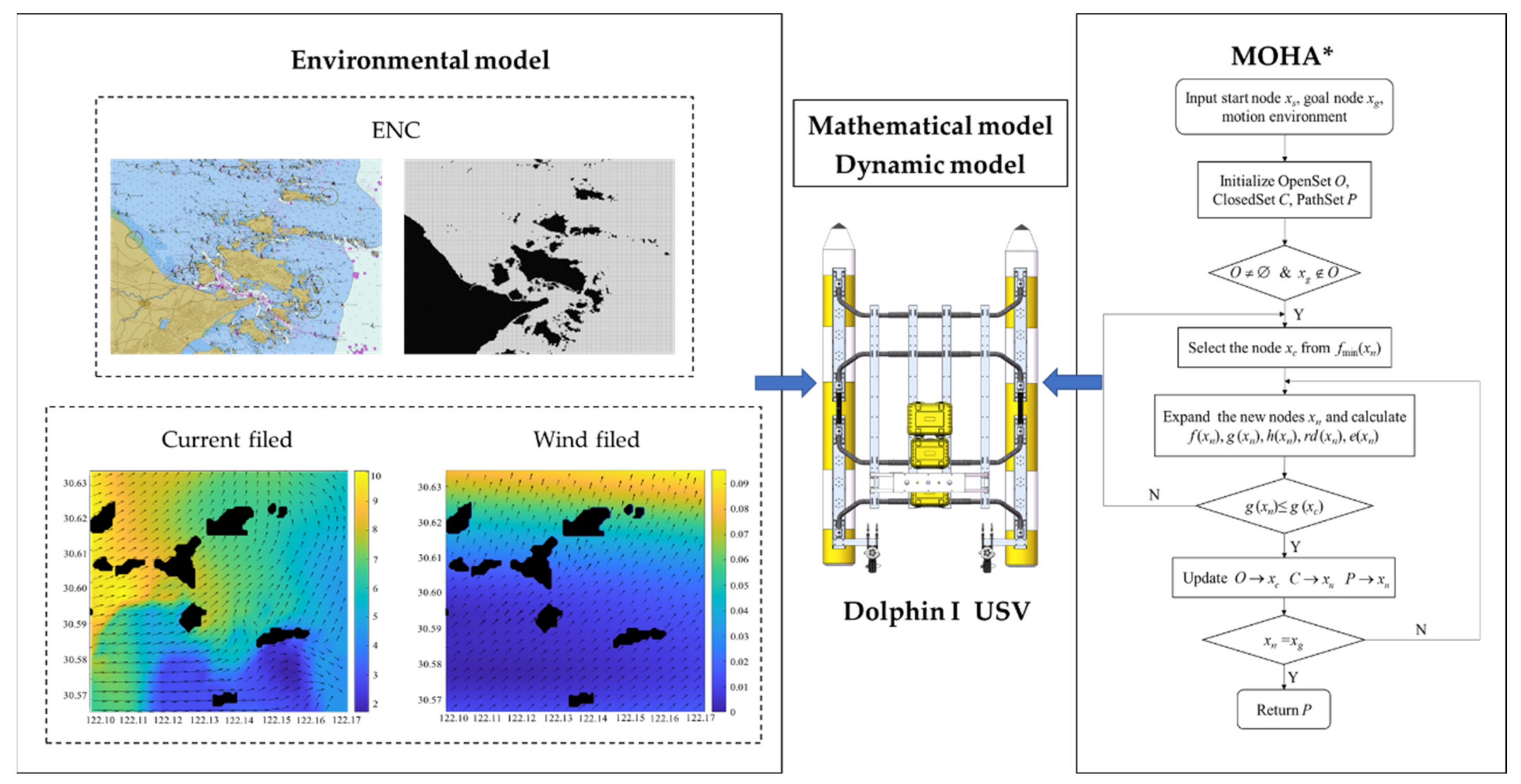
2.1. Construction of Navigation Environment Based on ENC
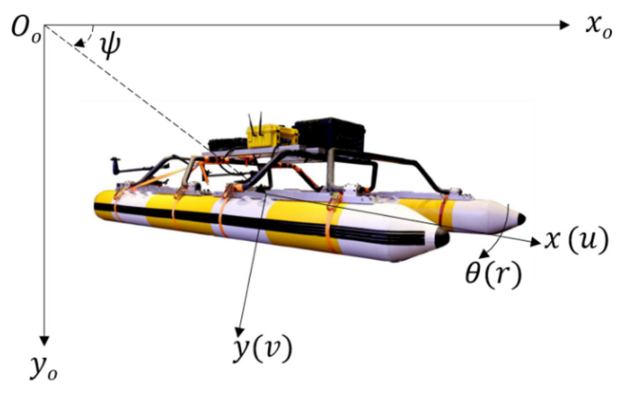
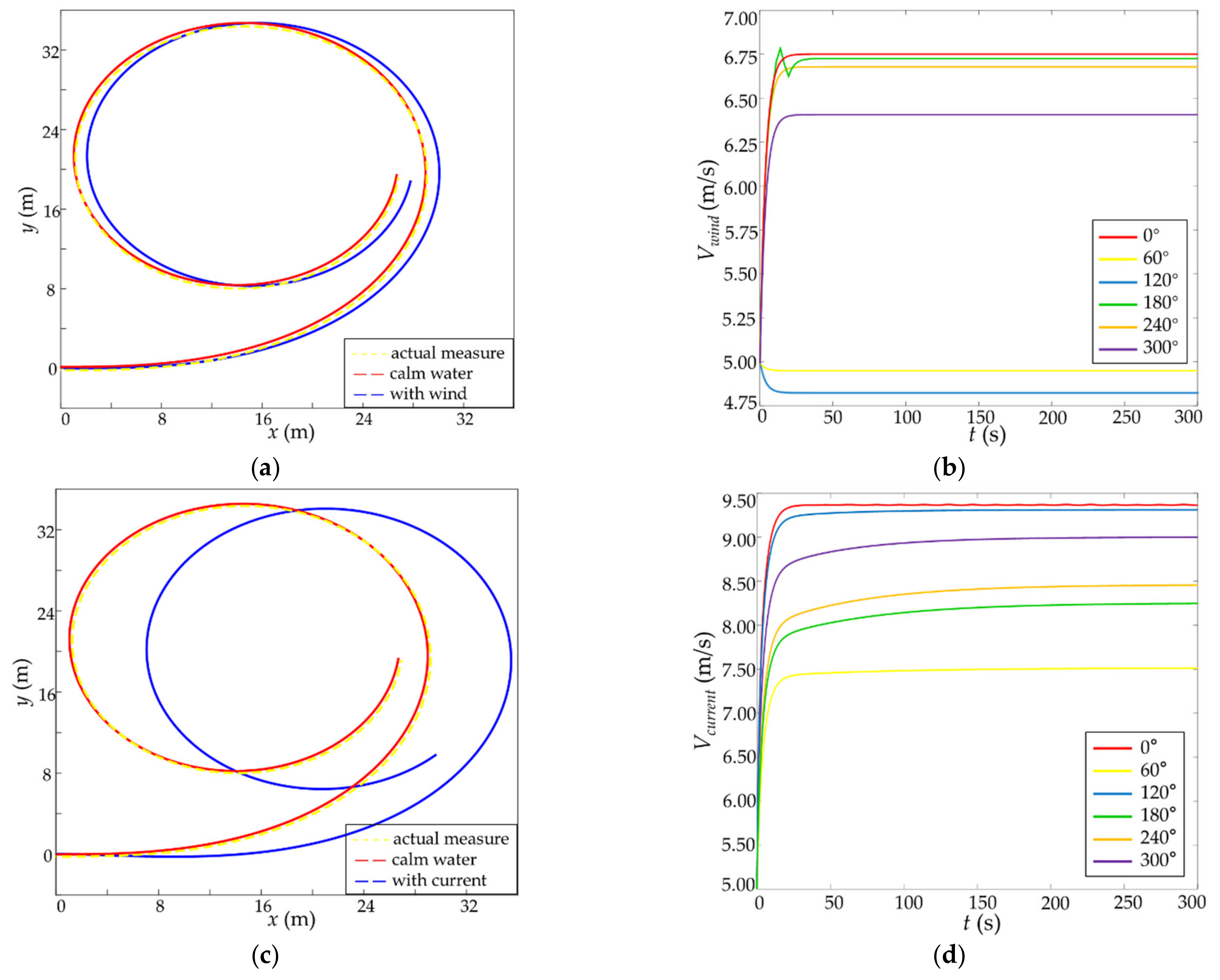
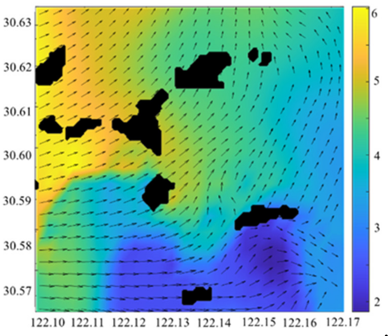
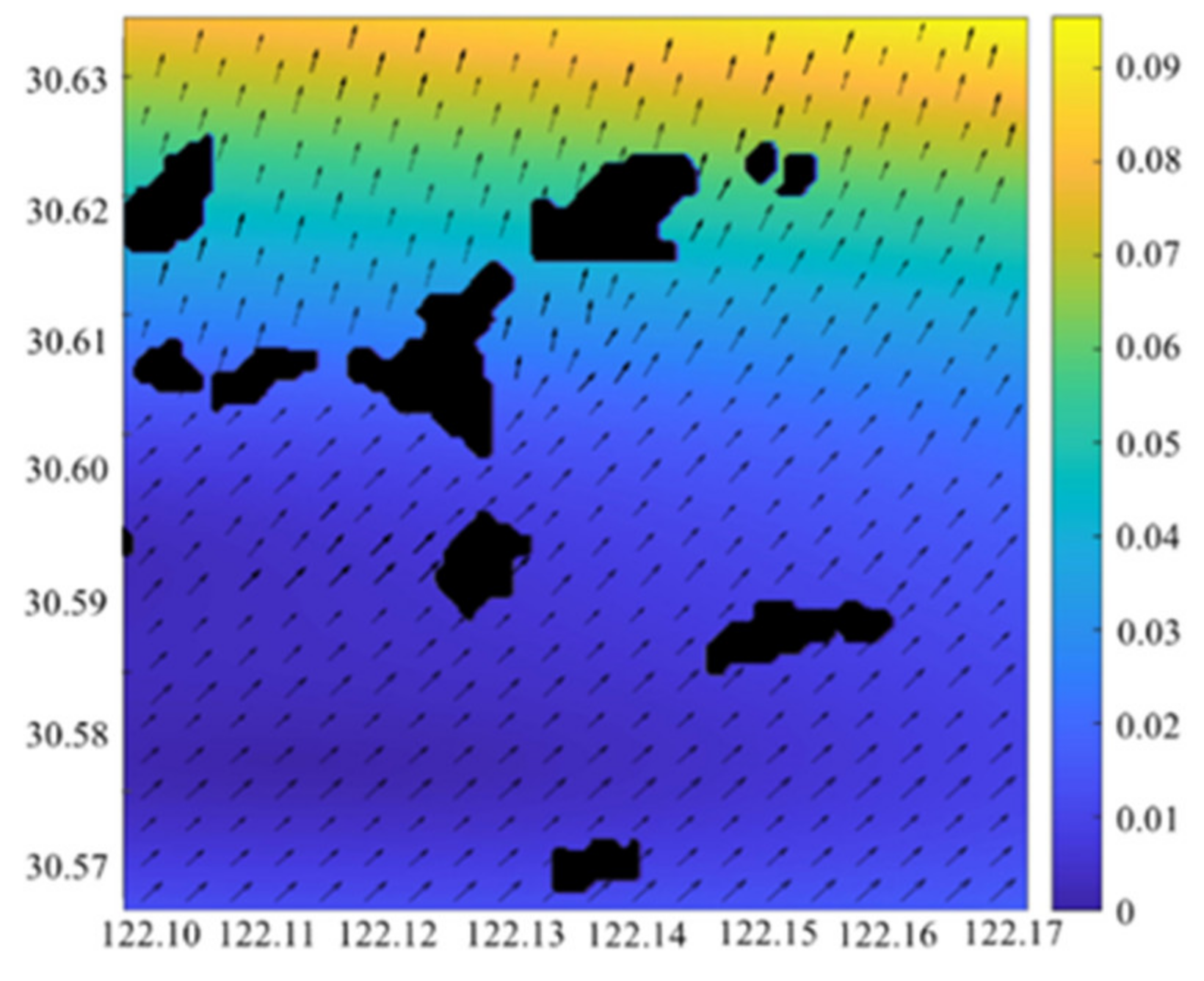
2.2. Mathematical Model of USV under the Influence of Wind and Current
2.3. Dynamic Model of USV under the Influence of Wind and Current
3. Algorithm of Ship Motion Planning
3.1. Traditional Hybrid A* Algorithm
3.2. Multi-Objective Optimization Model of USV Motion Planning
3.2.1. Graph Expansion/Search Model Based on Hybrid Motion Primitives
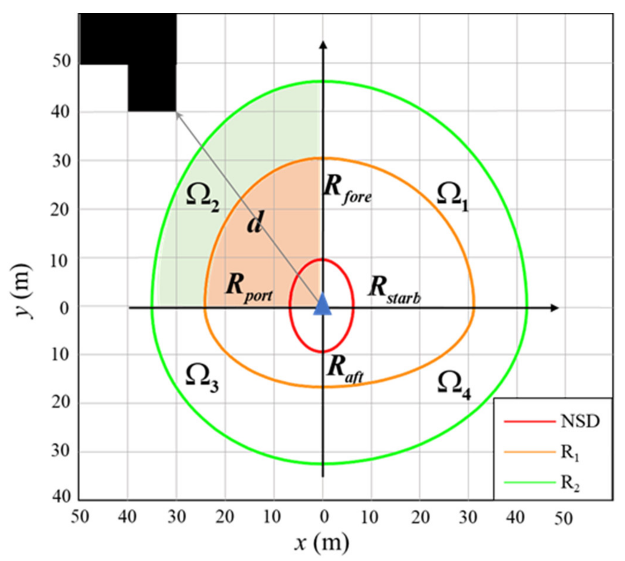
3.2.2. Risk Degree of Navigation Model Based on Ship Domain
3.2.3. Energy Consumption Model Based on Dynamic Analysis
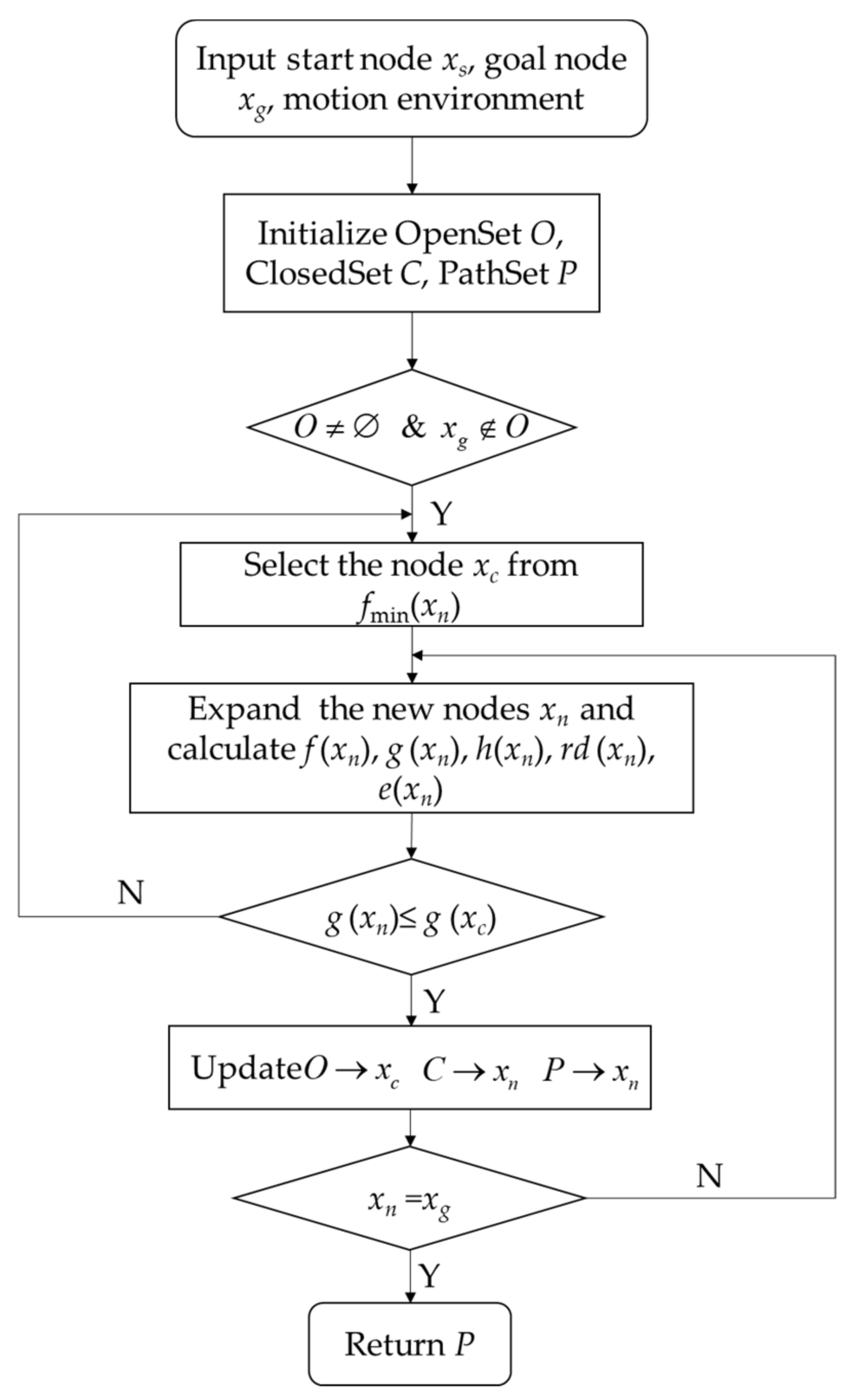
3.3. Multi-Objective Optimization Algorithm for Ship Motion Planning Based on HA*
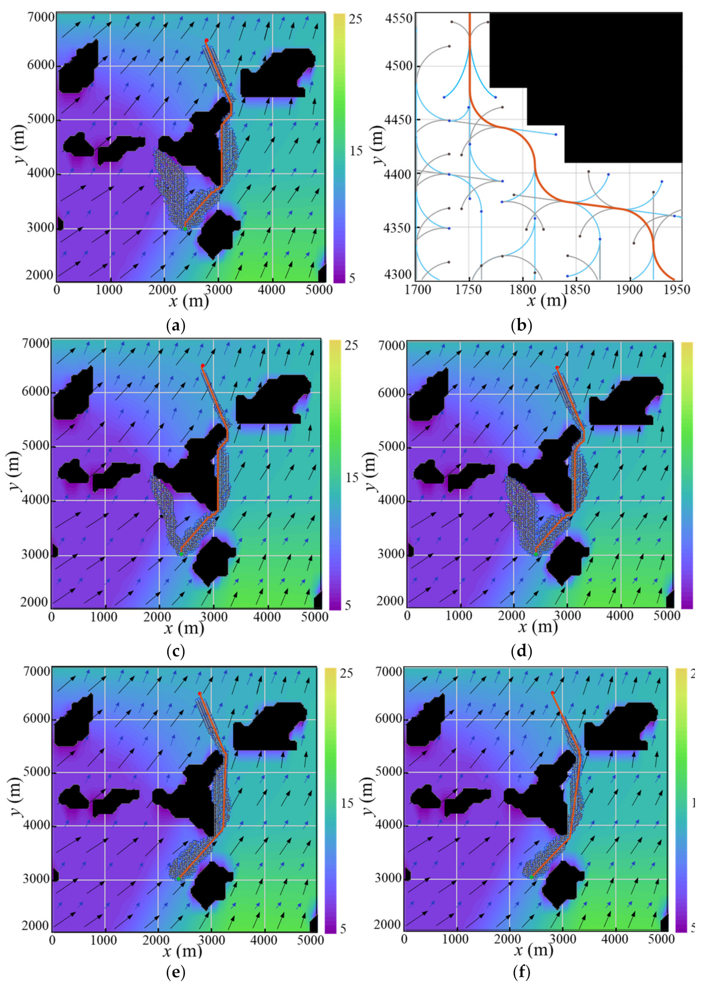
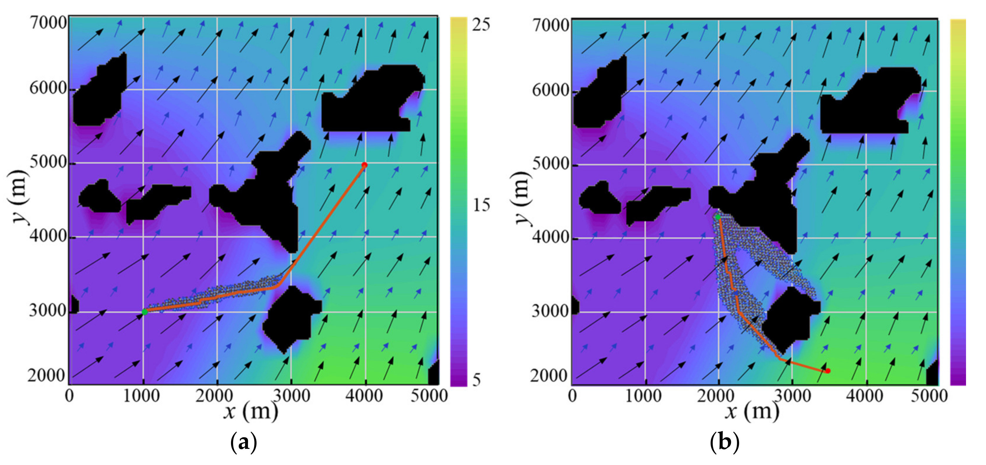
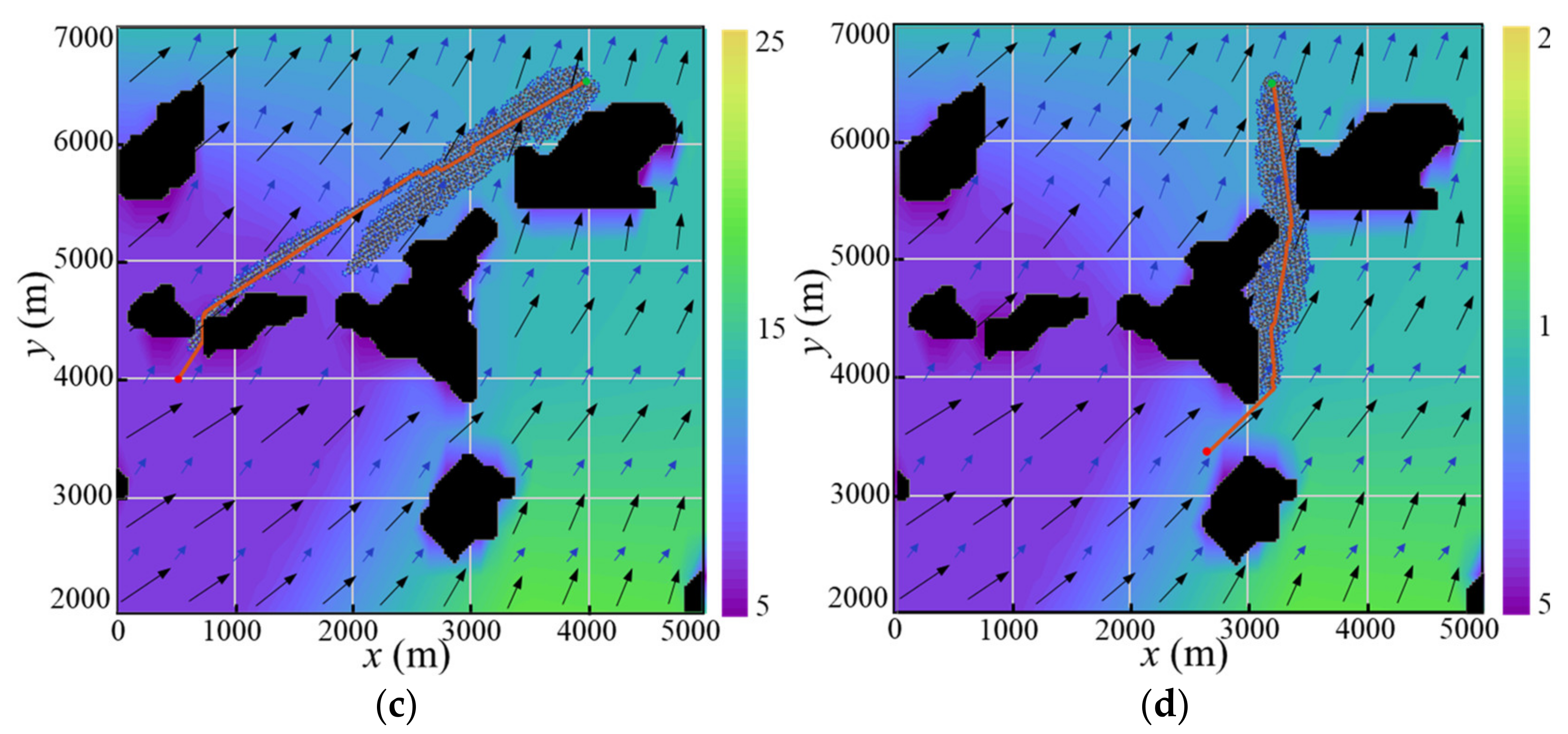
4. Simulation
5. Conclusions
Author Contributions
Funding
Institutional Review Board Statement
Informed Consent Statement
Data Availability Statement
Acknowledgments
Conflicts of Interest
References
- Liu, Y.; Bucknall, R. A survey of formation control and motion planning of multiple unmanned vehicles. Robotica 2018, 36, 1019–1047. [Google Scholar] [CrossRef]
- Zhou, C.; Gu, S.; Wen, Y.; Du, Z.; Xiao, C.; Huang, L.; Zhu, M. The review unmanned surface vehicle path planning: Based on multi-modality constraint. Ocean Eng. 2020, 200, 107043. [Google Scholar] [CrossRef]
- Macharet, D.G.; Campos, M.F.M. A survey on routing problems and robotic systems. Robotica 2018, 36, 1781–1803. [Google Scholar] [CrossRef]
- Liu, Z.; Zhang, Y.; Yu, X.; Yuan, C. Unmanned surface vehicles: An overview of developments and challenges. Annu. Rev. Control 2016, 41, 71–93. [Google Scholar] [CrossRef]
- European Maritime Safety Agency. Annual Overview of Marine Casualties and Incidents 2020 Publication; European Maritime Safety Agency: Lisbon, Portugal, 2020. [Google Scholar]
- Gao, M.; Shi, G.-Y.; Liu, J. Ship encounter azimuth map division based on automatic identification system data and support vector classification. Ocean Eng. 2020, 213. [Google Scholar] [CrossRef]
- Zhou, C.; Gu, S.; Wen, Y.; Du, Z.; Xiao, C.; Huang, L.; Zhu, M. Motion planning for an unmanned surface vehicle based on topological position maps. Ocean Eng. 2020, 198, 106798. [Google Scholar] [CrossRef]
- Liu, Y.; Bucknall, R. Path planning algorithm for unmanned surface vehicle formations in a practical maritime environment. Ocean Eng. 2015, 97, 126–144. [Google Scholar] [CrossRef]
- Gasparetto, A.; Boscariol, P.; Lanzutti, A.; Vidoni, R. Path Planning and Trajectory Planning Algorithms: A General Overview. In Motion and Operation Planning of Robotic Systems; Mechanisms and Machine Science; Springer International Publishing: Berlin, Germany, 2015; pp. 3–27. [Google Scholar]
- Shimoda, S.; Kuroda, Y.; Iagnemma, K. Potential field navigation of high speed unmanned ground vehicles on uneven terrain. In Proceedings of the IEEE International Conference on Robotics and Automation, Barcelona, Spain, 18–22 April 2005; pp. 2828–2833. [Google Scholar]
- Du, Z.; Wen, Y.; Xiao, C.; Zhang, F.; Huang, L.; Zhou, C. Motion planning for Unmanned Surface Vehicle based on Trajectory Unit. Ocean Eng. 2018, 151, 46–56. [Google Scholar] [CrossRef]
- Mohanan, M.G.; Salgoankar, A. A survey of robotic motion planning in dynamic environments. Robot. Auton. Syst. 2018, 100, 171–185. [Google Scholar] [CrossRef]
- Zaccone, R. COLREG-Compliant Optimal Path Planning for Real-Time Guidance and Control of Autonomous Ships. J. Mar. Sci. Eng. 2021, 9, 405. [Google Scholar] [CrossRef]
- Gonzalez, D.; Perez, J.; Milanes, V.; Nashashibi, F. A Review of Motion Planning Techniques for Automated Vehicles. IEEE Trans. Intell. Transp. Syst. 2016, 17, 1135–1145. [Google Scholar] [CrossRef]
- Lee, T.; Kim, H.; Chung, H.; Bang, Y.; Myung, H. Energy efficient path planning for a marine surface vehicle considering heading angle. Ocean Eng. 2015, 107, 118–131. [Google Scholar] [CrossRef]
- Vettor, R.; Guedes Soares, C. Development of a ship weather routing system. Ocean Eng. 2016, 123, 1–14. [Google Scholar] [CrossRef]
- Touzout, W.; Benmoussa, Y.; Benazzouz, D.; Moreac, E.; Diguet, J.-P. Unmanned surface vehicle energy consumption modelling under various realistic disturbances integrated into simulation environment. Ocean Eng. 2021, 222, 108560. [Google Scholar] [CrossRef]
- Huang, S.; Liu, W.; Luo, W.; Wang, K. Numerical Simulation of the Motion of a Large Scale Unmanned Surface Vessel in High Sea State Waves. J. Mar. Sci. Eng. 2021, 9, 982. [Google Scholar] [CrossRef]
- Ma, Y.; Hu, M.; Yan, X. Multi-objective path planning for unmanned surface vehicle with currents effects. ISA Trans. 2018, 75, 137–156. [Google Scholar] [CrossRef] [PubMed]
- Zaccone, R.; Martelli, M. A random sampling based algorithm for ship path planning with obstacles. In Proceedings of the International Ship Control Systems Symposium (iSCSS), Glasgow, UK, 2–4 October 2018. [Google Scholar]
- Koubaa, A.; Bennaceur, H.; Chaari, I.; Trigui, S.; Ammar, A. Robot Path Planning and Cooperation Foundations, Algorithms and Experimentations; Springer International Publishing: Cham, Switzerland, 2018. [Google Scholar]
- Sang, H.; You, Y.; Sun, X.; Zhou, Y.; Liu, F. The hybrid path planning algorithm based on improved A* and artificial potential field for unmanned surface vehicle formations. Ocean Eng. 2021, 223, 108709. [Google Scholar] [CrossRef]
- Liu, Y.; Bucknall, R. Efficient multi-task allocation and path planning for unmanned surface vehicle in support of ocean operations. Neurocomputing 2018, 275, 1550–1566. [Google Scholar] [CrossRef]
- Zuo, L.; Guo, Q.; Xu, X.; Fu, H. A hierarchical path planning approach based on A* and least-squares policy iteration for mobile robots. Neurocomputing 2015, 170, 257–266. [Google Scholar] [CrossRef]
- Han, D.-H.; Kim, Y.-D.; Lee, J.-Y. Multiple-criterion shortest path algorithms for global path planning of unmanned combat vehicles. Comput. Ind. Eng. 2014, 71, 57–69. [Google Scholar] [CrossRef]
- Subramani, D.N.; Lermusiaux, P.F.J. Energy-optimal path planning by stochastic dynamically orthogonal level-set optimization. Ocean Model. 2016, 100, 57–77. [Google Scholar] [CrossRef] [Green Version]
- Xu, H.; Rong, H.; Guedes Soares, C. Use of AIS data for guidance and control of path-following autonomous vessels. Ocean Eng. 2019, 194. [Google Scholar] [CrossRef]
- Xie, L.; Xue, S.; Zhang, J.; Zhang, M.; Tian, W.; Haugen, S. A path planning approach based on multi-direction A* algorithm for ships navigating within wind farm waters. Ocean Eng. 2019, 184, 311–322. [Google Scholar] [CrossRef]
- Xu, H.; Oliveira, P.; Guedes Soares, C. L1 adaptive backstepping control for path-following of underactuated marine surface ships. Eur. J. Control 2021, 58, 357–372. [Google Scholar] [CrossRef]
- Xu, H.; Fossen, T.I.; Guedes Soares, C. Uniformly semiglobally exponential stability of vector field guidance law and autopilot for path-following. Eur. J. Control 2020, 53, 88–97. [Google Scholar] [CrossRef]
- Zaccone, R.; Ottaviani, E.; Figari, M.; Altosole, M. Ship voyage optimization for safe and energy-efficient navigation: A dynamic programming approach. Ocean Eng. 2018, 153, 215–224. [Google Scholar] [CrossRef]
- Palikaris, A.; Mavraeidopoulos, A.K. Electronic Navigational Charts: International Standards and Map Projections. J. Mar. Sci. Eng. 2020, 8, 248. [Google Scholar] [CrossRef] [Green Version]
- Song, R.; Liu, Y.; Bucknall, R. Smoothed A* algorithm for practical unmanned surface vehicle path planning. Appl. Ocean Res. 2019, 83, 9–20. [Google Scholar] [CrossRef]
- Li, B.; Liu, H.; Su, W. Topology optimization techniques for mobile robot path planning. Appl. Soft Comput. 2019, 78, 528–544. [Google Scholar] [CrossRef]
- Niu, H.; Savvaris, A.; Tsourdos, A.; Ji, Z. Voronoi-Visibility Roadmap-based Path Planning Algorithm for Unmanned Surface Vehicles. J. Navig. 2019, 72, 850–874. [Google Scholar] [CrossRef]
- Blasi, L.; D’Amato, E.; Mattei, M.; Notaro, I. Path Planning and Real-Time Collision Avoidance Based on the Essential Visibility Graph. Appl. Sci. 2020, 10, 5613. [Google Scholar] [CrossRef]
- Yu, K.; Liang, X.-f.; Li, M.-z.; Chen, Z.; Yao, Y.-l.; Li, X.; Zhao, Z.-x.; Teng, Y. USV path planning method with velocity variation and global optimisation based on AIS service platform. Ocean Eng. 2021, 236, 109560. [Google Scholar] [CrossRef]
- Marie, S.; Courteille, E. Multi-Objective Optimization of Motor Vessel Route. Int. J. Mar. Navig. Saf. Sea Transp. 2009, 3, 133–141. [Google Scholar]
- Becker, E.; Chen, M.; Wang, W.; Zhang, Q.; van den Dool, H.; Mendez, M.P.; Yang, R.; Meng, J.; Ek, M.; Iredell, M.; et al. The NCEP Climate Forecast System Version 2. J. Clim. 2014, 27, 2185–2208. [Google Scholar] [CrossRef]
- Zhai, F.; Wang, Q.; Wang, F.; Hu, D. Variation of the North Equatorial Current, Mindanao Current, and Kuroshio Current in a high-resolution data assimilation during 2008–2012. Adv. Atmos. Sci. 2014, 31, 1445–1459. [Google Scholar] [CrossRef]
- Chassignet, E.P.; Hurlburt, H.E.; Smedstad, O.M.; Halliwell, G.R.; Hogan, P.J.; Wallcraft, A.J.; Baraille, R.; Bleck, R. The HYCOM (HYbrid Coordinate Ocean Model) data assimilative system. J. Mar. Syst. 2007, 65, 60–83. [Google Scholar] [CrossRef]
- Chen, Z.; Wang, X.; Liu, L. Reconstruction of Three-Dimensional Ocean Structure From Sea Surface Data: An Application of isQG Method in the Southwest Indian Ocean. J. Geophys. Res. Ocean. 2020, 125. [Google Scholar] [CrossRef]
- Cummings, J.A. Operational multivariate ocean data assimilation. Q. J. R. Meteorol. Soc. 2005, 131, 3583–3604. [Google Scholar] [CrossRef] [Green Version]
- You, X.; Ma, F.; Huang, M.; He, W. Study on the MMG three-degree-of-freedom motion model of a sailing vessel. In Proceedings of the 2017 4th International Conference on Transportation Information and Safety (ICTIS), Banff, AB, Canada, 8–10 August 2017. [Google Scholar]
- Fan, J.; Li, Y.; Liao, Y.; Jiang, W.; Wang, L.; Jia, Q.; Wu, H. Second Path Planning for Unmanned Surface Vehicle Considering the Constraint of Motion Performance. J. Mar. Sci. Eng. 2019, 7, 104. [Google Scholar] [CrossRef] [Green Version]
- Yasukawa, H.; Yoshimura, Y. Introduction of MMG standard method for ship maneuvering predictions. J. Mar. Sci. Technol. 2014, 20, 37–52. [Google Scholar] [CrossRef] [Green Version]
- Jin, J.; Zhang, J.; Liu, D. Design and Verification of Heading and Velocity Coupled Nonlinear Controller for Unmanned Surface Vehicle. Sensors 2018, 18, 3427. [Google Scholar] [CrossRef] [Green Version]
- Li, C.; Jiang, J.; Duan, F.; Liu, W.; Wang, X.; Bu, L.; Sun, Z.; Yang, G. Modeling and Experimental Testing of an Unmanned Surface Vehicle with Rudderless Double Thrusters. Sensors 2019, 19, 2051. [Google Scholar] [CrossRef] [Green Version]
- Isherwood, R. Wind resistance of merchant ships. R. Inst. Nav. Archit. 1972, 115, 327–338. [Google Scholar]
- Fossen, T.I. Handbook of Marine Craft Hydrodynamics and Motion Control; John Wiley & Sons: Chichester, UK, 2011. [Google Scholar]
- Vagale, A.; Oucheikh, R.; Bye, R.T.; Osen, O.L.; Fossen, T.I. Path planning and collision avoidance for autonomous surface vehicles I: A review. J. Mar. Sci. Technol. 2021. [Google Scholar] [CrossRef]
- Dolgov, D.; Thrun, S.; Montemerlo, M.; Diebel, J. Practical Search Techniques in Path Planning for Autonomous Driving. Ann Arbor 2008, 1001, 18–80. [Google Scholar]
- Mannarini, G.; Subramani, D.N.; Lermusiaux, P.F.J.; Pinardi, N. Graph-Search and Differential Equations for Time-Optimal Vessel Route Planning in Dynamic Ocean Waves. IEEE Trans. Intell. Transp. Syst. 2020, 21, 3581–3593. [Google Scholar] [CrossRef] [Green Version]
- Wang, N. A Novel Analytical Framework for Dynamic Quaternion Ship Domains. J. Navig. 2012, 66, 265–281. [Google Scholar] [CrossRef] [Green Version]
- Deng, F.; Jin, L.; Hou, X.; Wang, L.; Li, B.; Yang, H. COLREGs: Compliant Dynamic Obstacle Avoidance of USVs Based on theDynamic Navigation Ship Domain. J. Mar. Sci. Eng. 2021, 9, 837. [Google Scholar] [CrossRef]
- Wang, N. An Intelligent Spatial Collision Risk Based on the Quaternion Ship Domain. J. Navig. 2010, 63, 733–749. [Google Scholar] [CrossRef]
- Zhou, J.; Wang, C.; Zhang, A. A COLREGs-Based Dynamic Navigation Safety Domain for Unmanned Surface Vehicles: A Case Study of Dolphin-I. J. Mar. Sci. Eng. 2020, 8, 264. [Google Scholar] [CrossRef] [Green Version]
- Niu, H.; Ji, Z.; Savvaris, A.; Tsourdos, A. Energy efficient path planning for Unmanned Surface Vehicle in spatially-temporally variant environment. Ocean Eng. 2020, 196, 106766. [Google Scholar] [CrossRef]


| Types of Events | 2014 | 2015 | 2016 | 2017 | 2018 | 2019 | Percentage | |
|---|---|---|---|---|---|---|---|---|
| Capsizing/listing |  | 11 | 15 | 8 | 15 | 18 | 17 | 0.63% |
| Collision |  | 332 | 293 | 317 | 292 | 279 | 256 | 13.40% |
| Contact |  | 390 | 402 | 357 | 420 | 379 | 320 | 17.18% |
| Damage/loss of equipment |  | 287 | 361 | 356 | 310 | 341 | 297 | 14.78% |
| Fire/explosion |  | 160 | 173 | 131 | 133 | 133 | 124 | 6.47% |
| Flooding/foundering |  | 60 | 56 | 44 | 62 | 35 | 46 | 2.29% |
| Grounding/stranding |  | 325 | 329 | 290 | 292 | 301 | 228 | 13.36% |
| Hull failure |  | 6 | 15 | 22 | 5 | 5 | 4 | 0.43% |
| Loss of control |  | 589 | 572 | 680 | 751 | 759 | 796 | 31.40% |
| Index | Parameters |
|---|---|
| Length (m) | 3.2 |
| Breadth (m) | 2.2 |
| Weight (kg) | 120 |
| Draft (m) | 0.3–0.5 |
| Velocity (m/s) | 7.0 |
| Advance (m) | 16.5 |
| Diameter Tactical (m) | 24.5 |
| Motion Primitive | Length (m) | |K| |
|---|---|---|
 | 25 | 0.04 |
 | 30 | 0.026 |
 | 38 | 0.013 |
 | 25/30/38 | 0 |
| Test | Number of Nodes | Risk Degree | Time (s) | Energy (KJ) |
|---|---|---|---|---|
| 1 | 5450 | 46 | 14.56 | 4252 |
| 2 | 4164 | 46 | 11.16 | 4168 |
| 3 | 5477 | 27 | 14.73 | 4318 |
| 4 | 3742 | 43 | 9.78 | 3512 |
| 5 | 2987 | 22 | 7.57 | 3224 |
| Test | Start Position | Goal Position | Combination of Motion Primitives |
|---|---|---|---|
| 6 | (1000, 3000, π/4) | (4000, 5000, 0) | L1 + SL + SL + L1…M1 + M2 + L1 + SL |
| 7 | (2000, 4300, −π/2) | (3500, 2200, 0) | L2 + SL + M1 + S1…S1 + S2 + S1 + SL |
| 8 | (4000, 6500, 0) | (500, 4000, −π/4) | SL + L1 + L2 + L2…SL + M2 + S2 + S2 |
| 9 | (3200, 6500, 0) | (2500, 3400, −π/2) | M1 + M2 + M1 + S1…M1 + M2 + S2 + SL |
Publisher’s Note: MDPI stays neutral with regard to jurisdictional claims in published maps and institutional affiliations. |
© 2021 by the authors. Licensee MDPI, Basel, Switzerland. This article is an open access article distributed under the terms and conditions of the Creative Commons Attribution (CC BY) license (https://creativecommons.org/licenses/by/4.0/).
Share and Cite
Wu, M.; Zhang, A.; Gao, M.; Zhang, J. Ship Motion Planning for MASS Based on a Multi-Objective Optimization HA* Algorithm in Complex Navigation Conditions. J. Mar. Sci. Eng. 2021, 9, 1126. https://doi.org/10.3390/jmse9101126
Wu M, Zhang A, Gao M, Zhang J. Ship Motion Planning for MASS Based on a Multi-Objective Optimization HA* Algorithm in Complex Navigation Conditions. Journal of Marine Science and Engineering. 2021; 9(10):1126. https://doi.org/10.3390/jmse9101126
Chicago/Turabian StyleWu, Meiyi, Anmin Zhang, Miao Gao, and Jiali Zhang. 2021. "Ship Motion Planning for MASS Based on a Multi-Objective Optimization HA* Algorithm in Complex Navigation Conditions" Journal of Marine Science and Engineering 9, no. 10: 1126. https://doi.org/10.3390/jmse9101126
APA StyleWu, M., Zhang, A., Gao, M., & Zhang, J. (2021). Ship Motion Planning for MASS Based on a Multi-Objective Optimization HA* Algorithm in Complex Navigation Conditions. Journal of Marine Science and Engineering, 9(10), 1126. https://doi.org/10.3390/jmse9101126