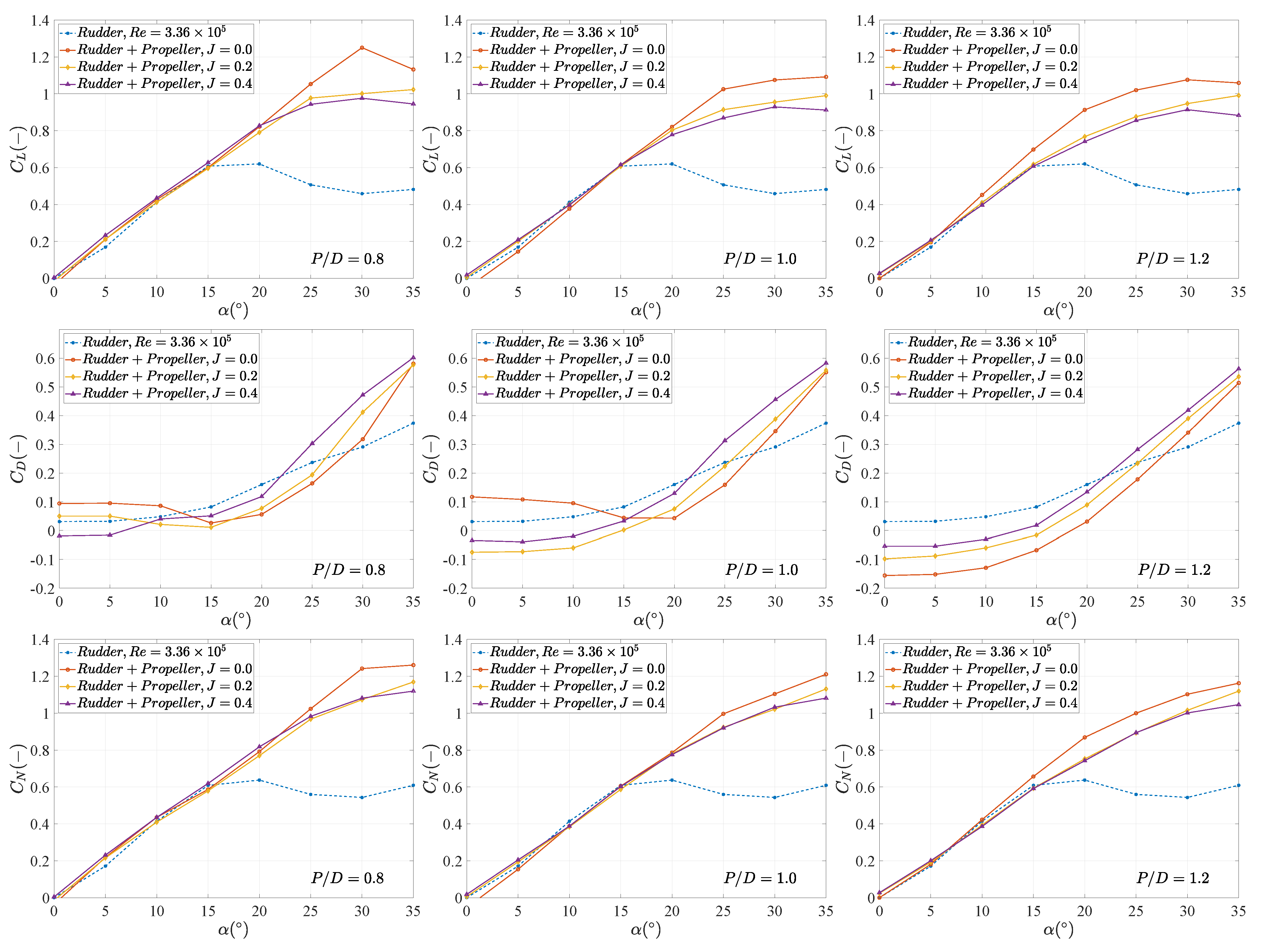
Figure 1.
Comparison of the hydrodynamic coefficients of a rudder in open water conditions to those of the rudder in propeller slipstream. Data are adopted from Nienhuis [
13].
Figure 1.
Comparison of the hydrodynamic coefficients of a rudder in open water conditions to those of the rudder in propeller slipstream. Data are adopted from Nienhuis [
13].
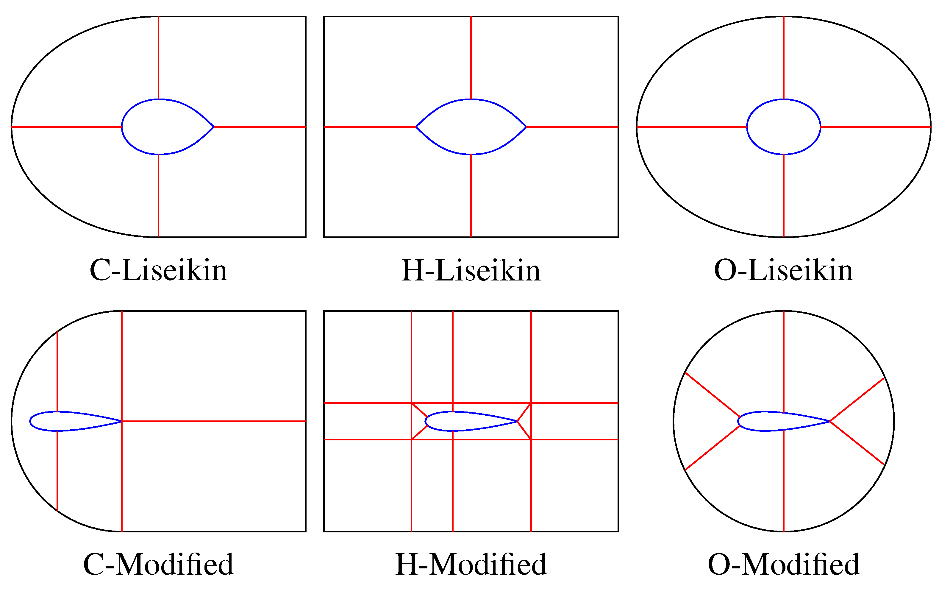
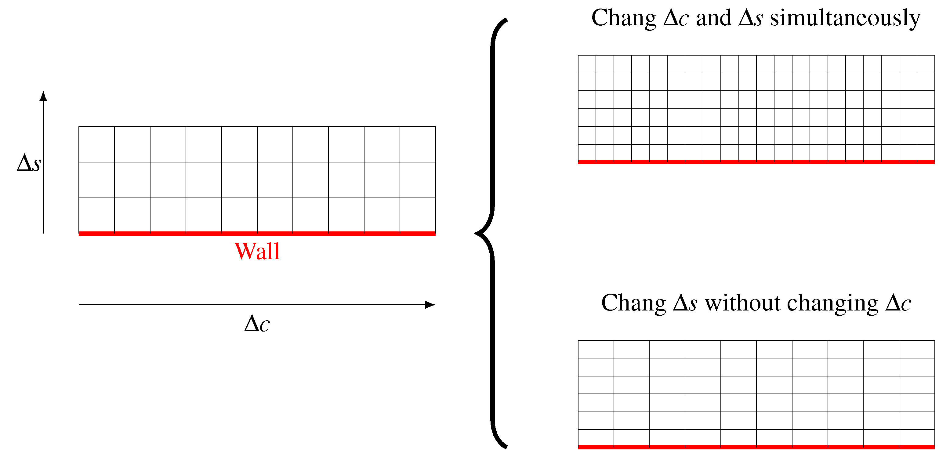
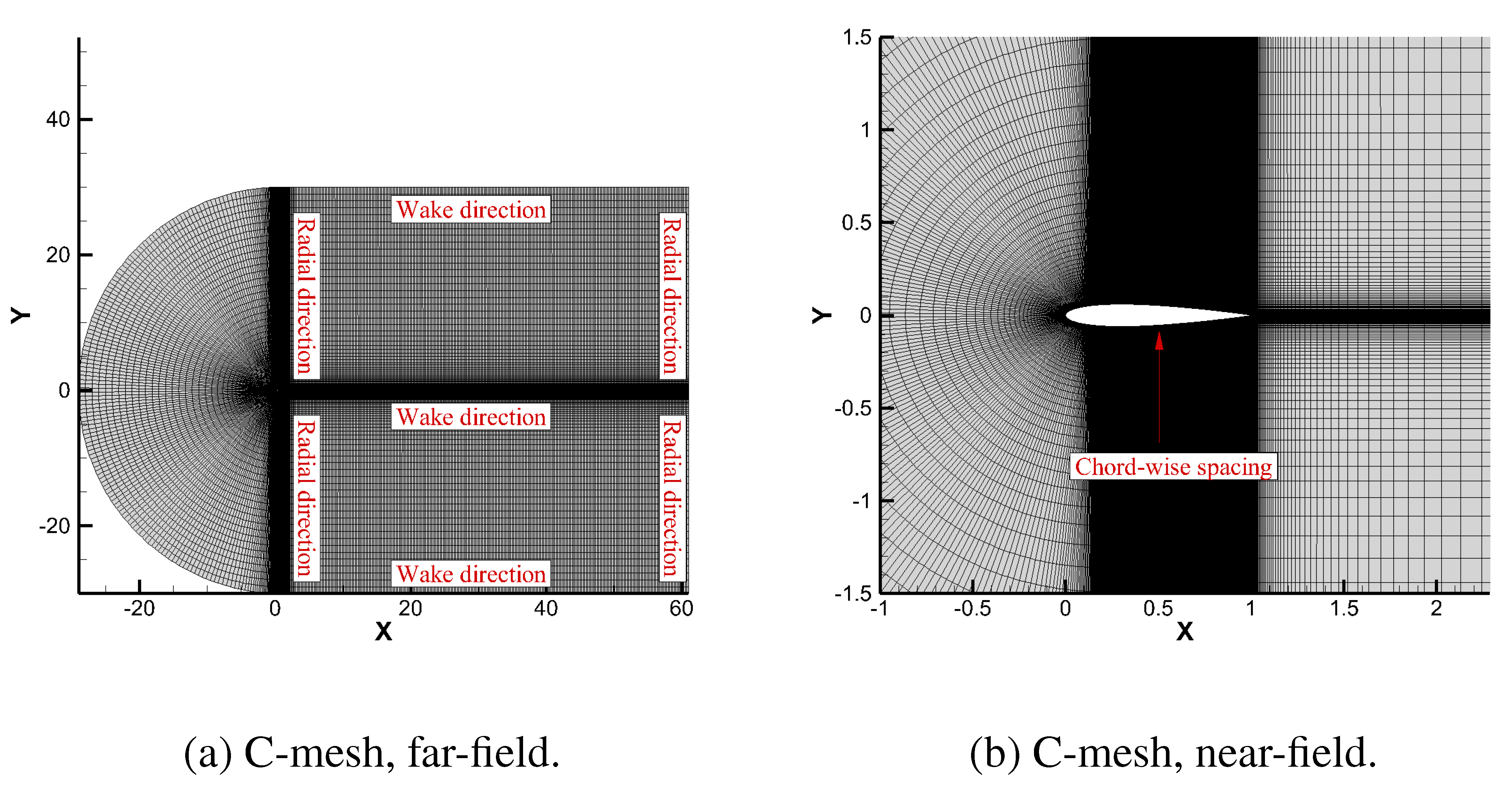
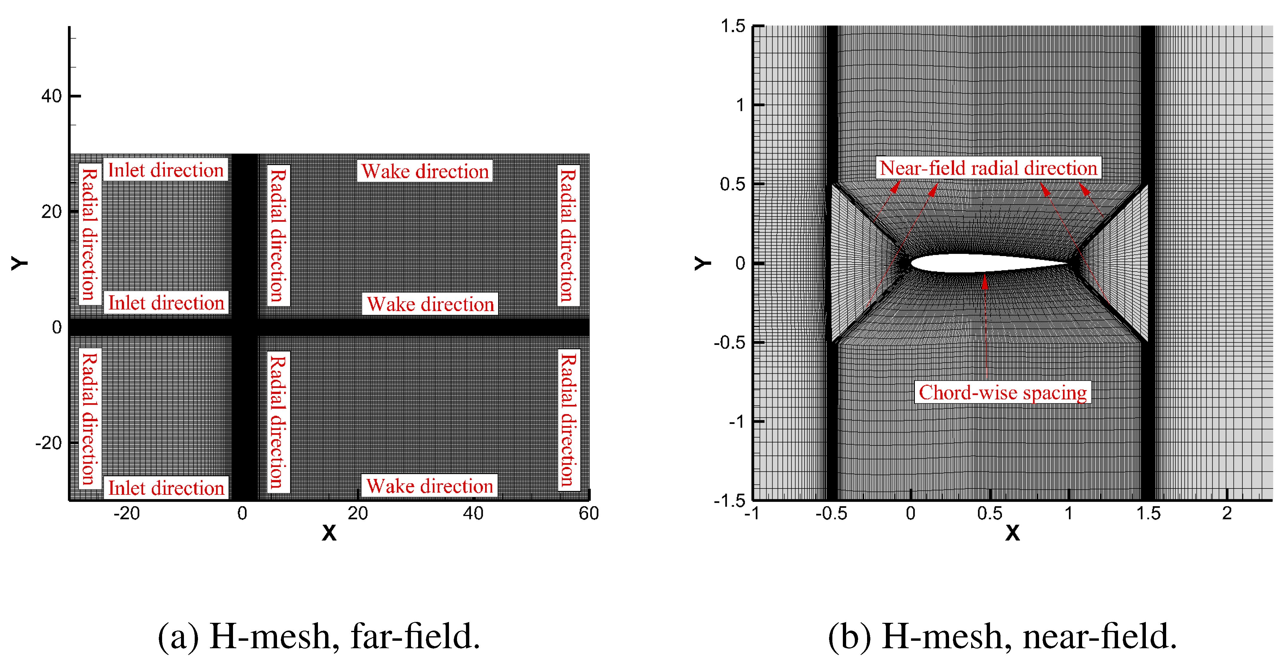
Figure 2.
Original and modified mesh types for the block-structured mesh.
Figure 2.
Original and modified mesh types for the block-structured mesh.
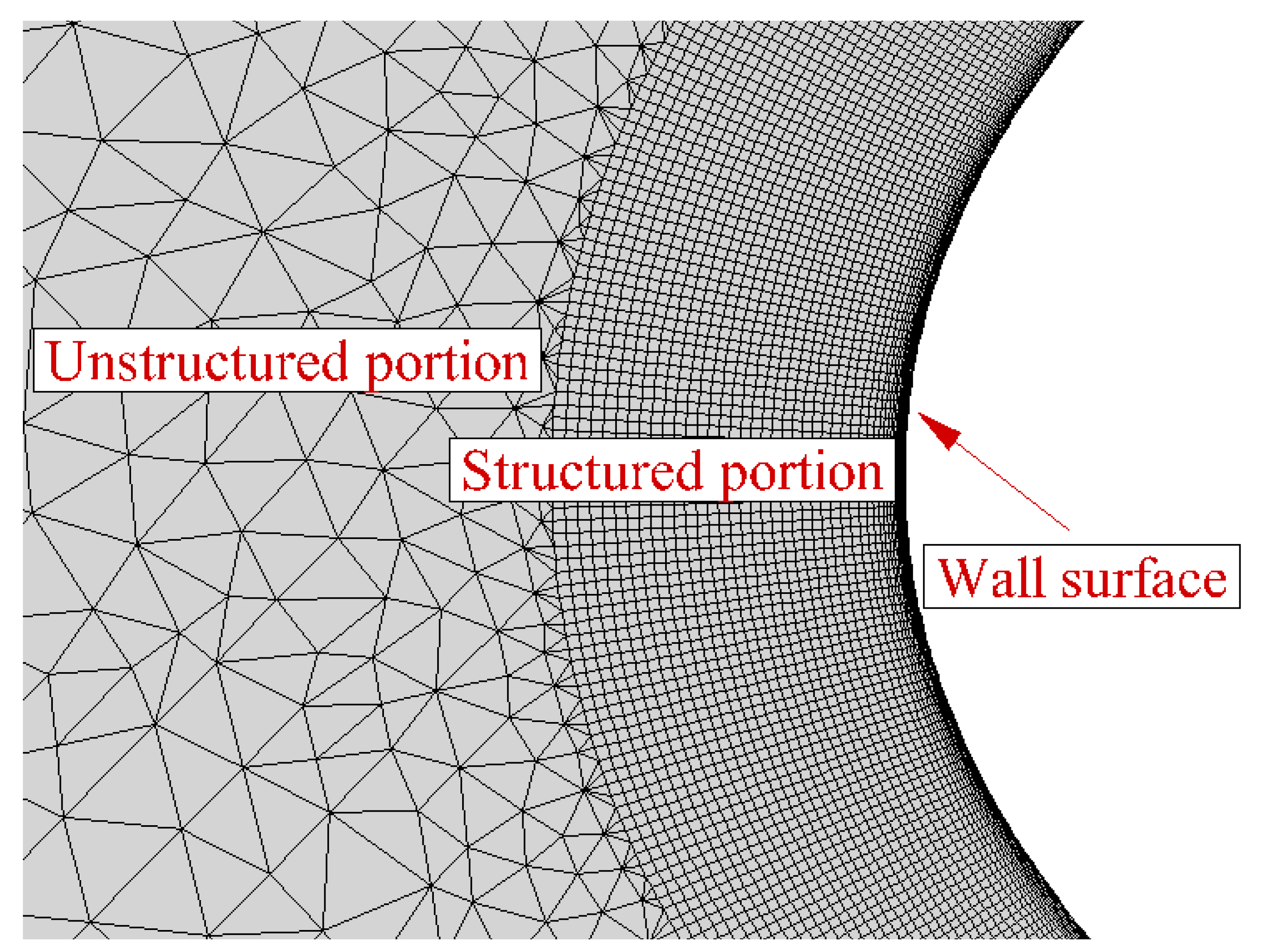
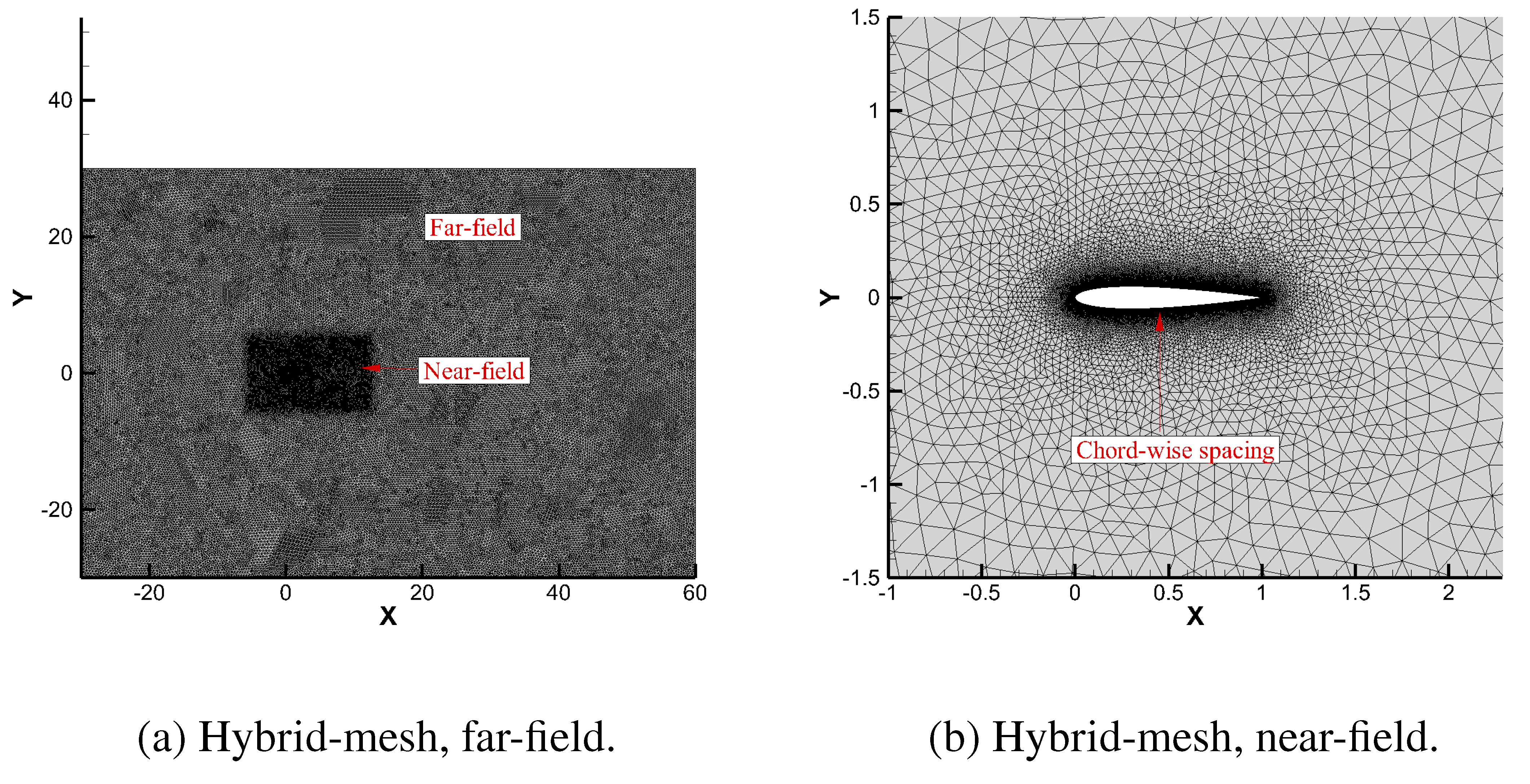
Figure 3.
The mesh type of Hybrid-mesh.
Figure 3.
The mesh type of Hybrid-mesh.
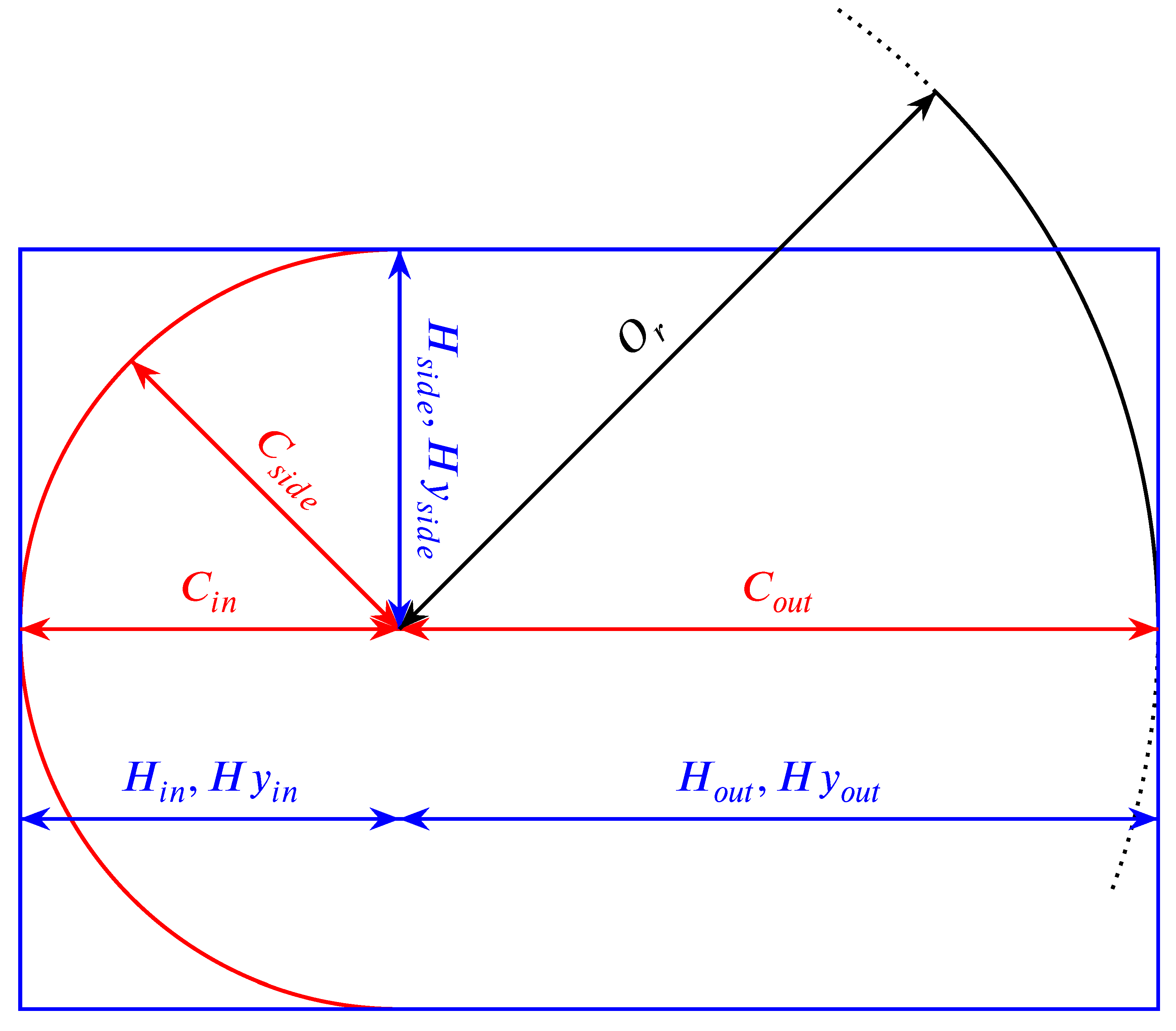
Figure 4.
The geometric parameters for different mesh types.
Figure 4.
The geometric parameters for different mesh types.
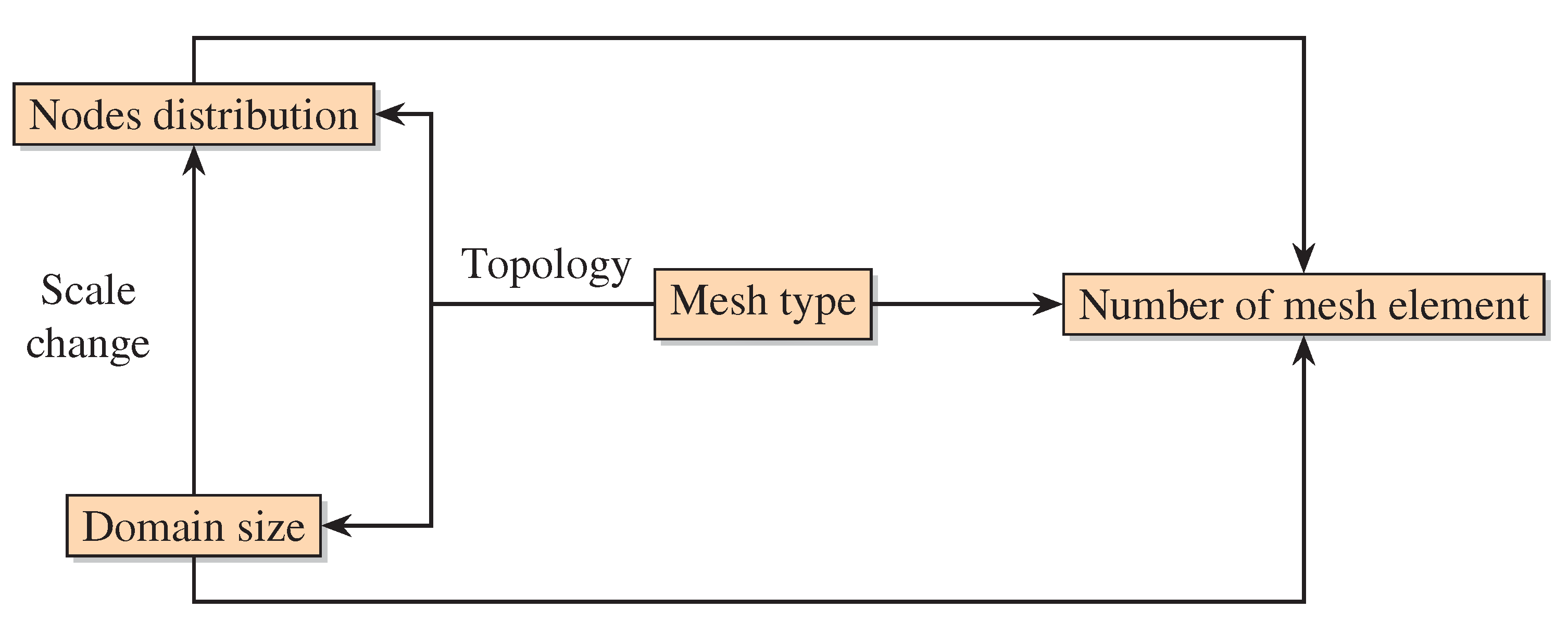
Figure 5.
Relationship between different mesh properties.
Figure 5.
Relationship between different mesh properties.
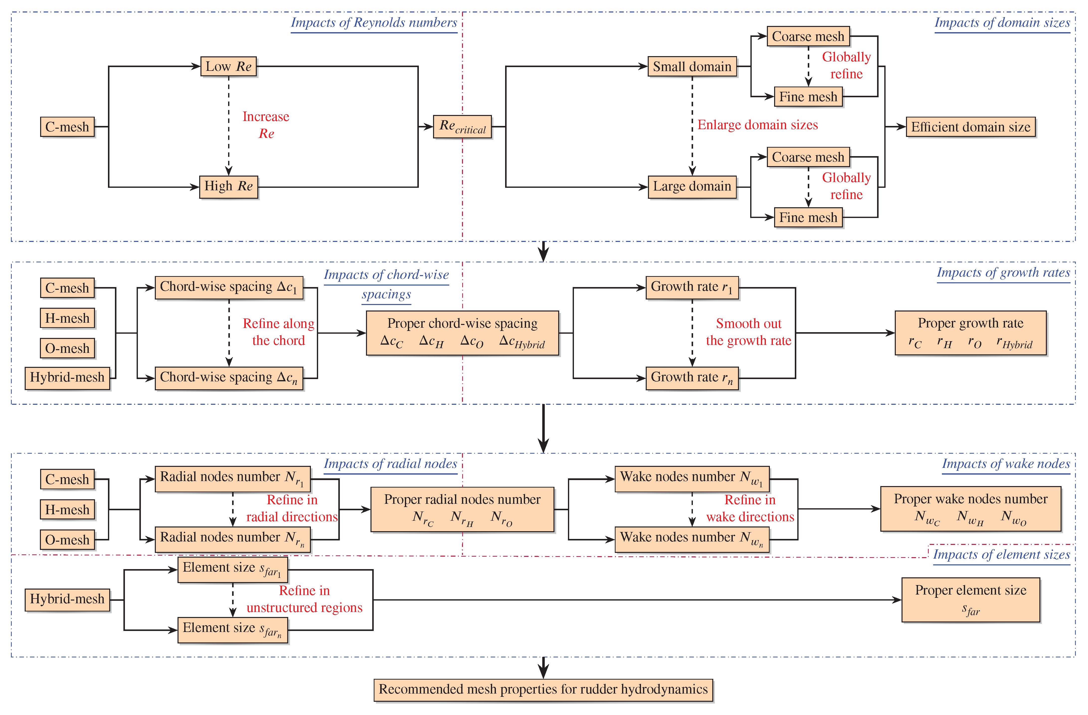
Figure 6.
Strategy applied to study different mesh properties.
Figure 6.
Strategy applied to study different mesh properties.
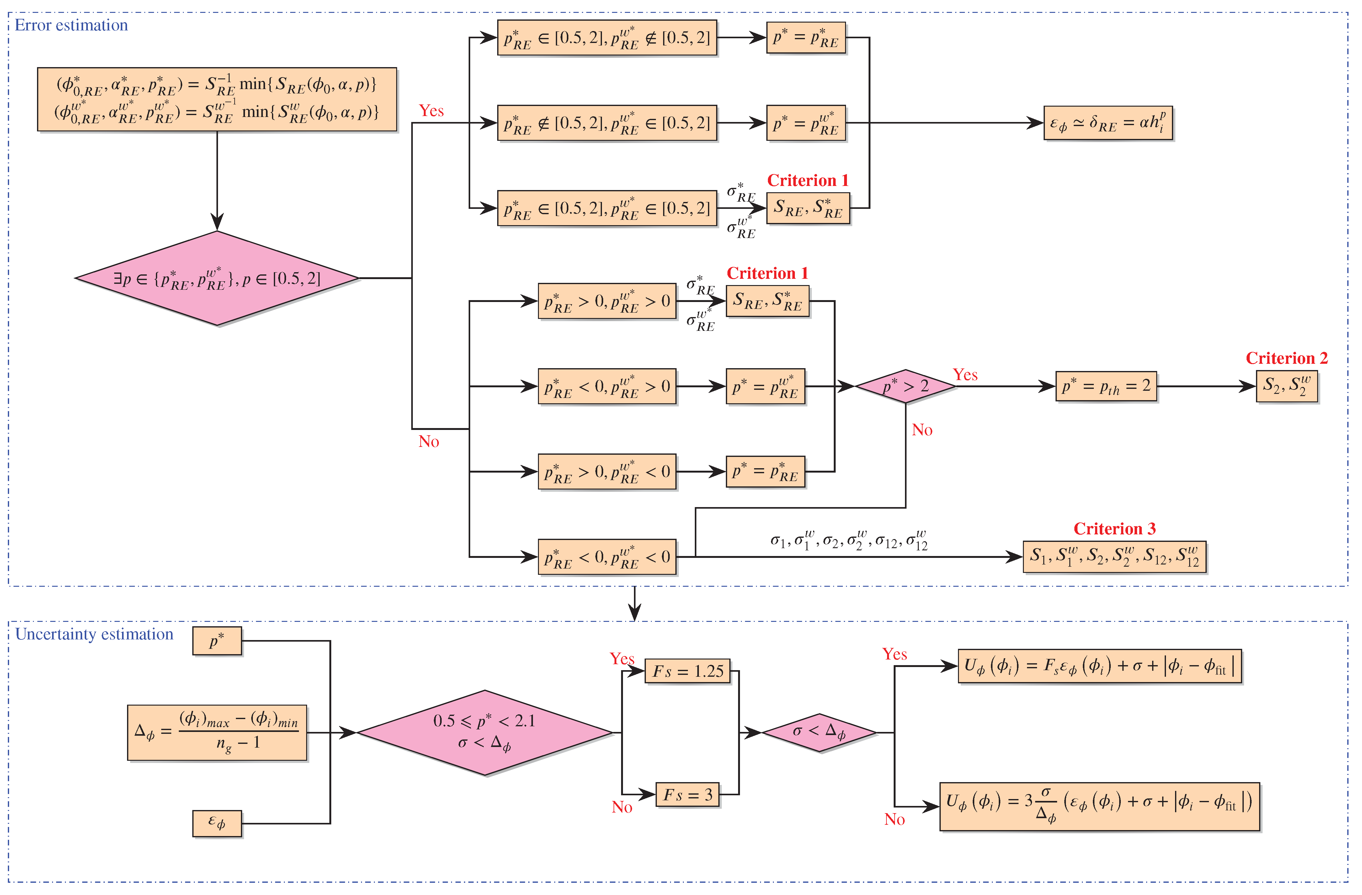
Figure 7.
Procedure for error and uncertainty estimations by GCI-LSR method recommended by Eça and Hoekstra [
31], De Luca et al. [
32].
Figure 7.
Procedure for error and uncertainty estimations by GCI-LSR method recommended by Eça and Hoekstra [
31], De Luca et al. [
32].
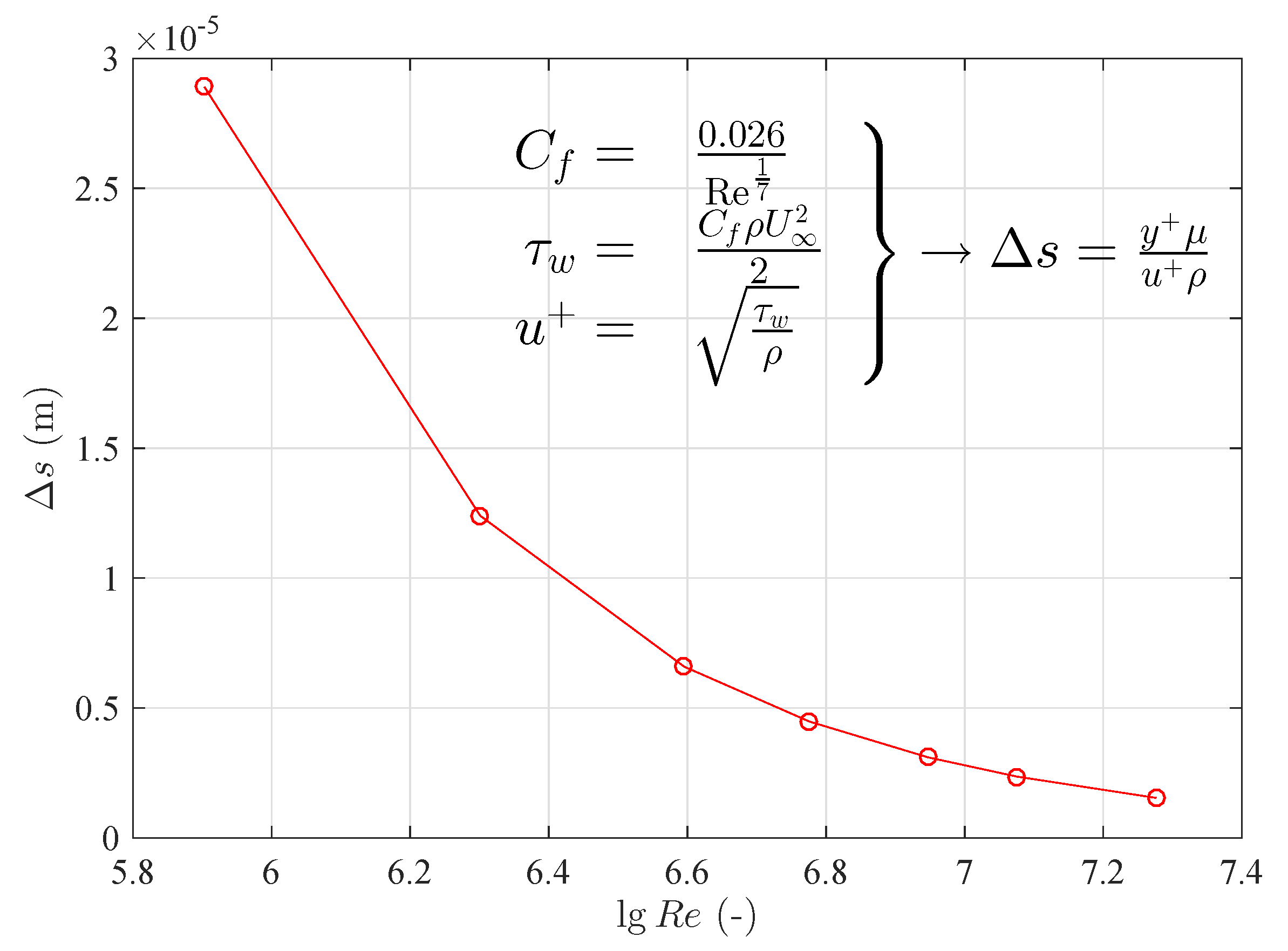
Figure 8.
Different meshes’ height of first layer with varying and .
Figure 8.
Different meshes’ height of first layer with varying and .
Figure 9.
Impacts of height of first mesh on aspects ratios.
Figure 9.
Impacts of height of first mesh on aspects ratios.
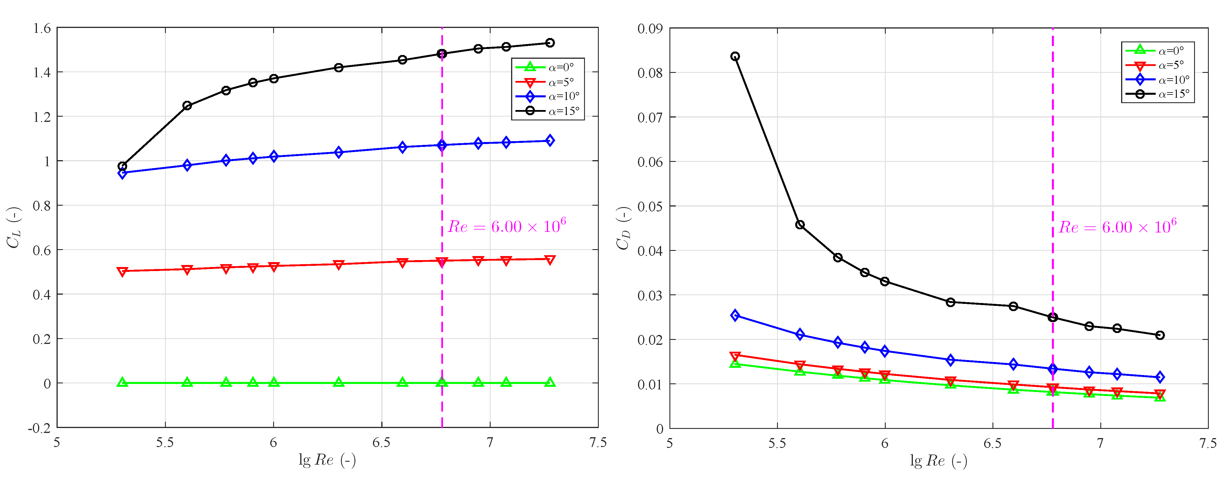
Figure 10.
Impacts of on lift and drag coefficients.
Figure 10.
Impacts of on lift and drag coefficients.
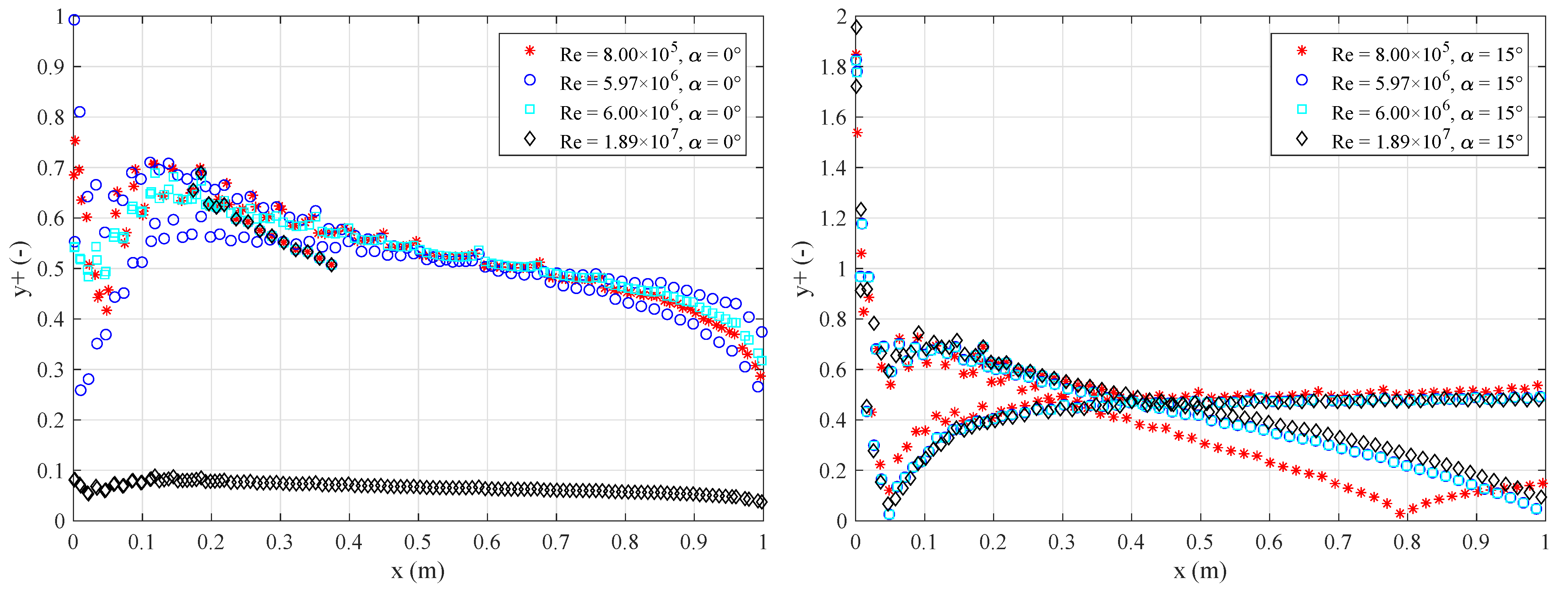
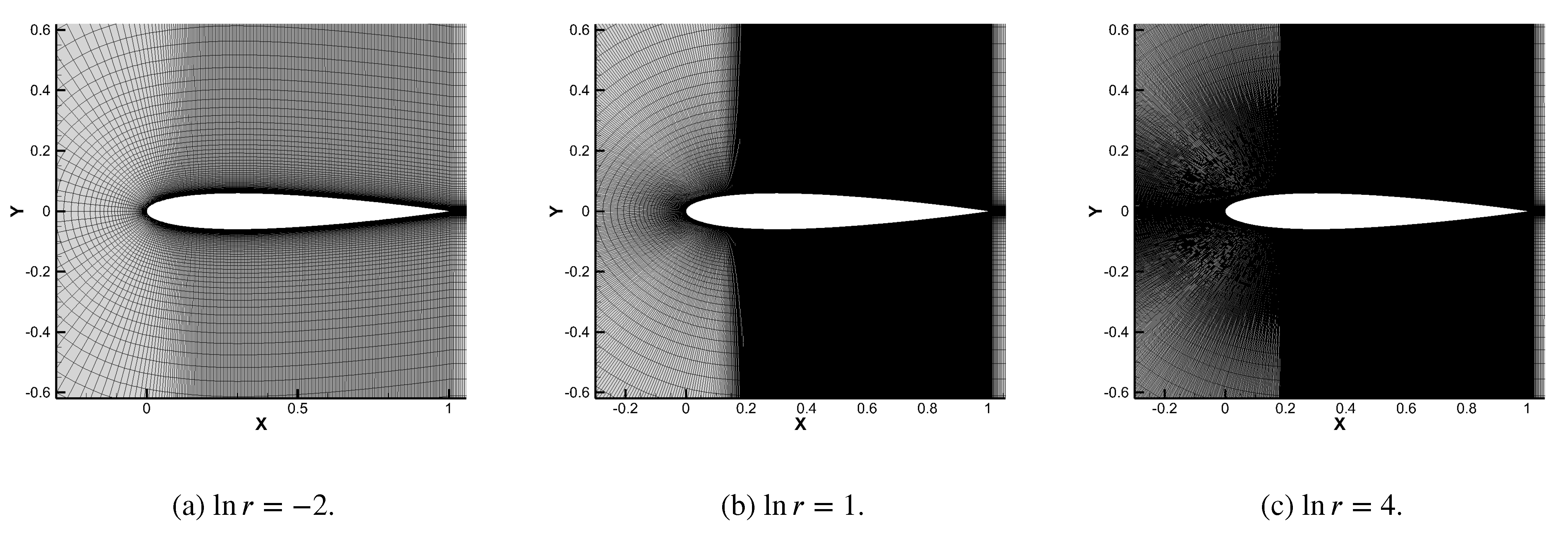
Figure 11.
along rudder chord with varying .
Figure 11.
along rudder chord with varying .
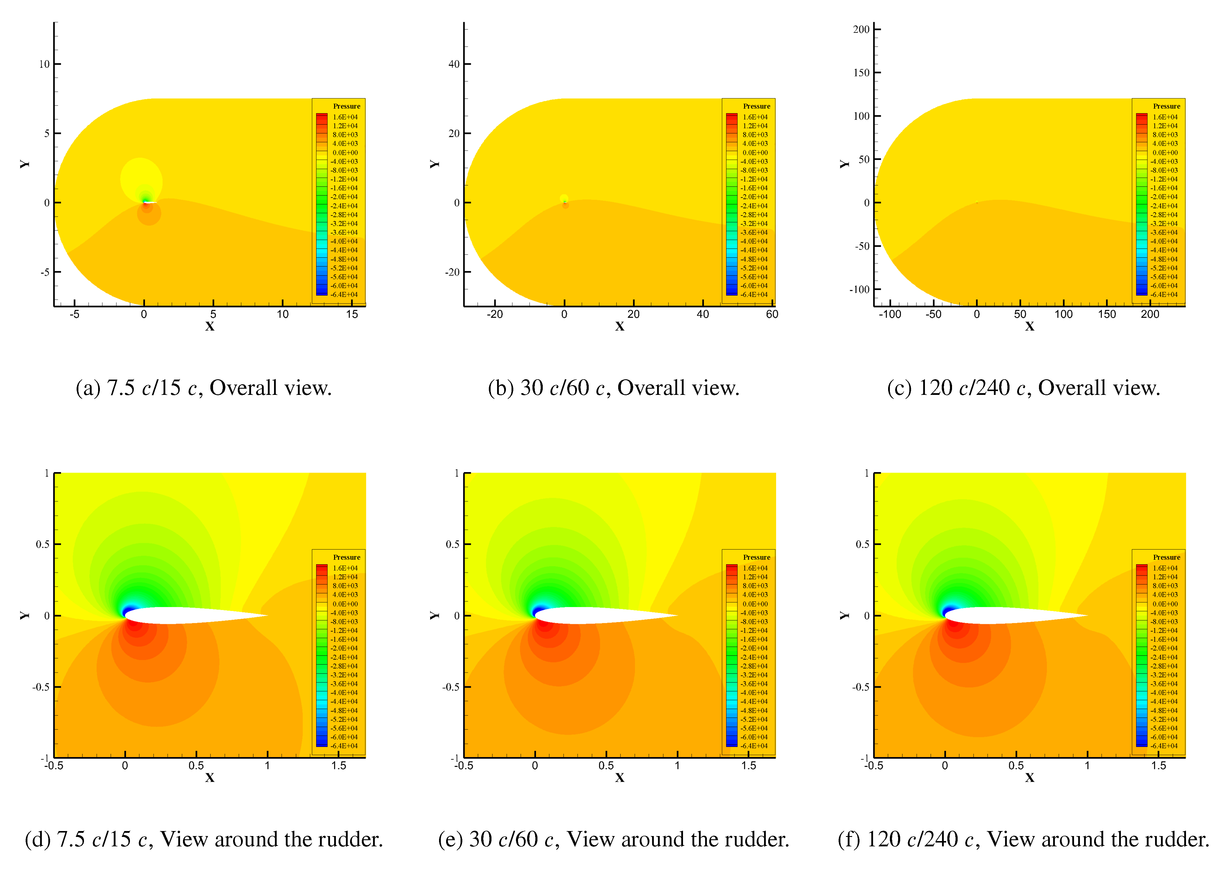
Figure 12.
Pressure contours of different domain sizes with .
Figure 12.
Pressure contours of different domain sizes with .
Figure 13.
Node distributions for C-mesh.
Figure 13.
Node distributions for C-mesh.
Figure 14.
Node distributions for H-mesh.
Figure 14.
Node distributions for H-mesh.
Figure 15.
Node distributions for O-mesh.
Figure 15.
Node distributions for O-mesh.
Figure 16.
Node distributions for Hybrid-mesh.
Figure 16.
Node distributions for Hybrid-mesh.
Figure 17.
Cells around the rudder with varying chord-wise spacings for C-mesh.
Figure 17.
Cells around the rudder with varying chord-wise spacings for C-mesh.
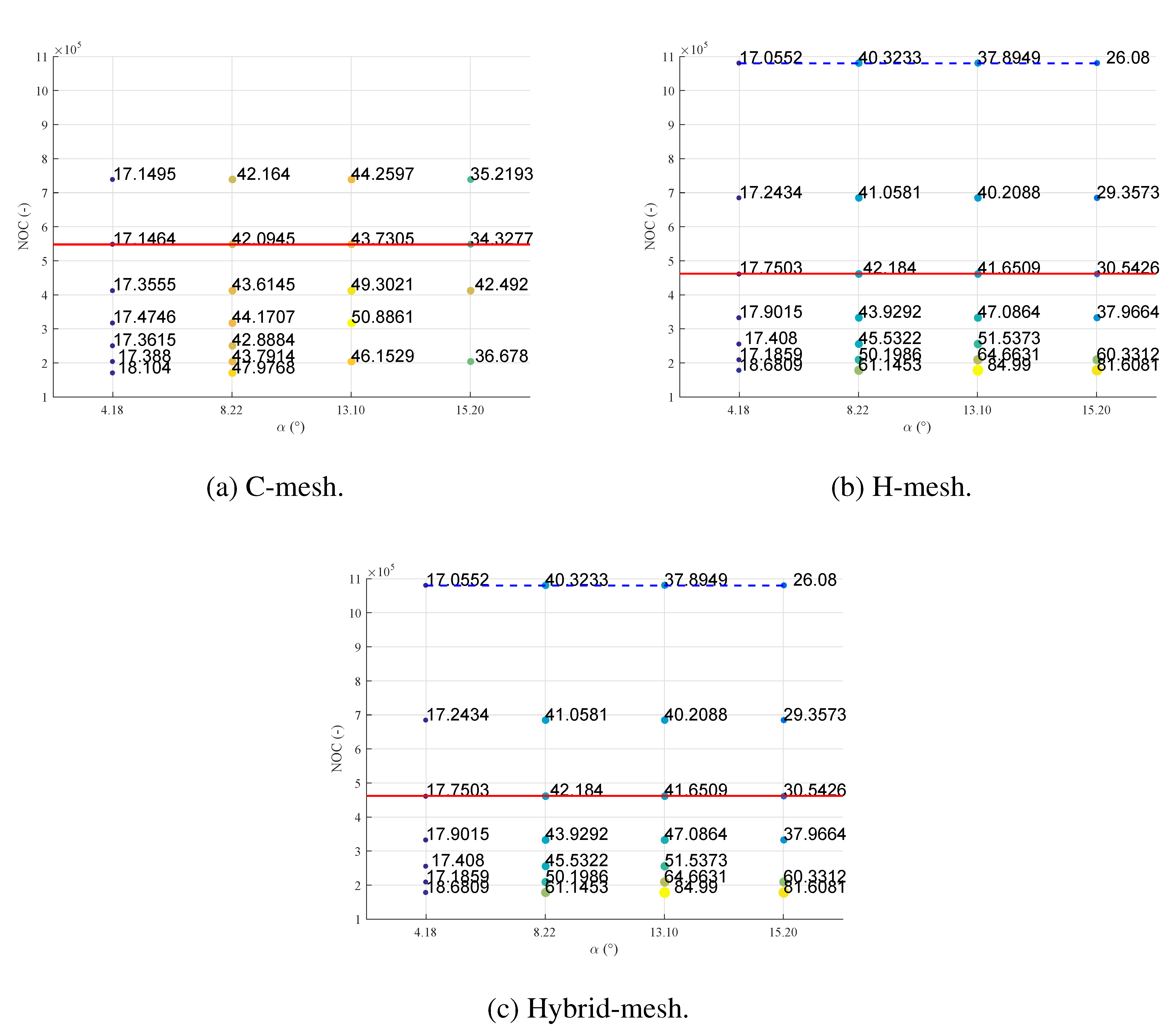
Figure 18.
Calculation deviations of
compared with experimental benchmark data adopted from [
25] varying with numbers of cells, while changing chord-wise spacings in the near-field (blue dotted lines connect minimum errors under each
and red lines mark selected mesh settings for each type).
Figure 18.
Calculation deviations of
compared with experimental benchmark data adopted from [
25] varying with numbers of cells, while changing chord-wise spacings in the near-field (blue dotted lines connect minimum errors under each
and red lines mark selected mesh settings for each type).
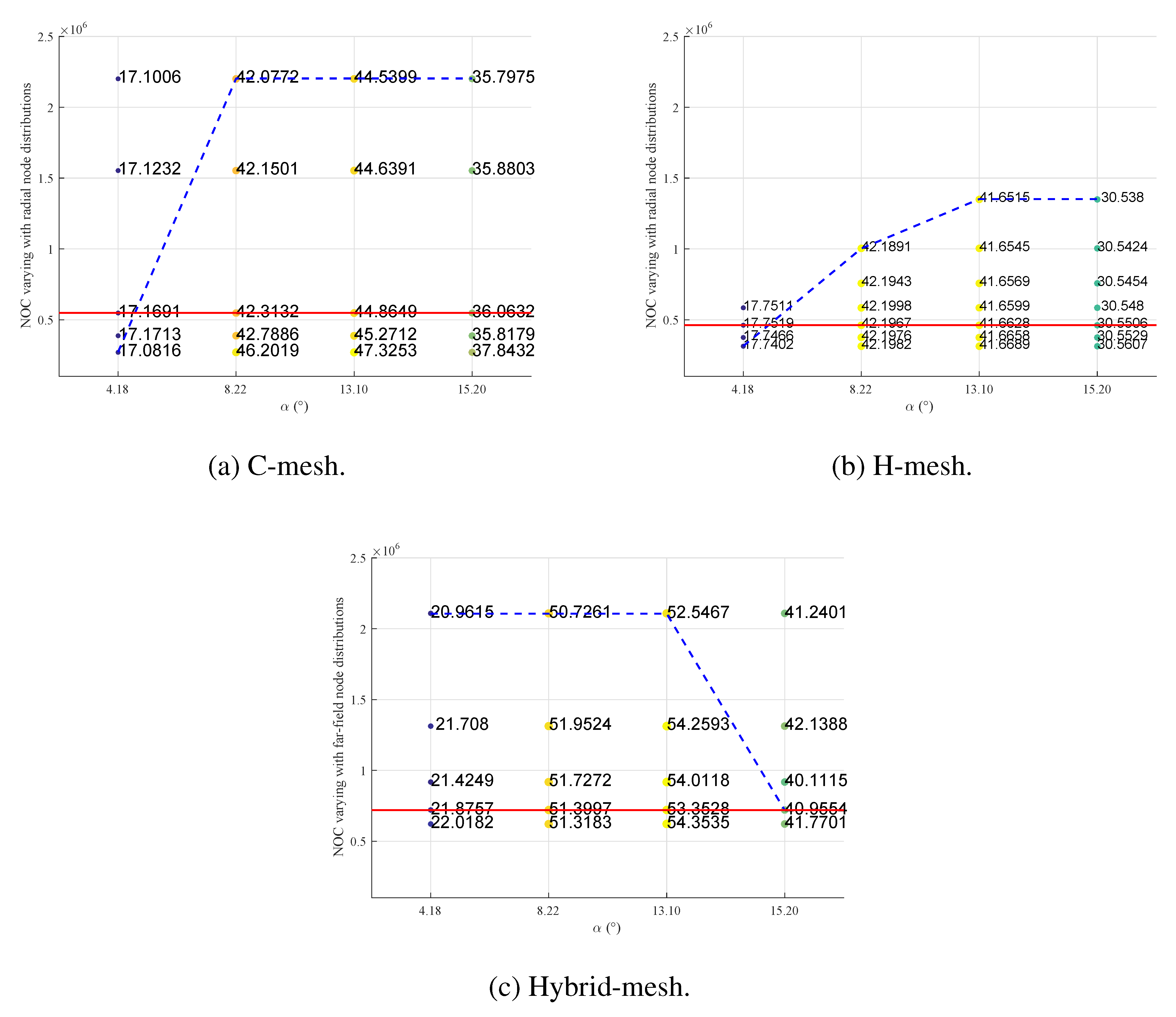
Figure 19.
Calculation deviations of
compared with experimental benchmark data adopted from [
25] varying with numbers of cells, while changing radial node distributions in near-field (blue dotted lines connect minimum errors under each
and red lines mark selected mesh settings for each type).
Figure 19.
Calculation deviations of
compared with experimental benchmark data adopted from [
25] varying with numbers of cells, while changing radial node distributions in near-field (blue dotted lines connect minimum errors under each
and red lines mark selected mesh settings for each type).
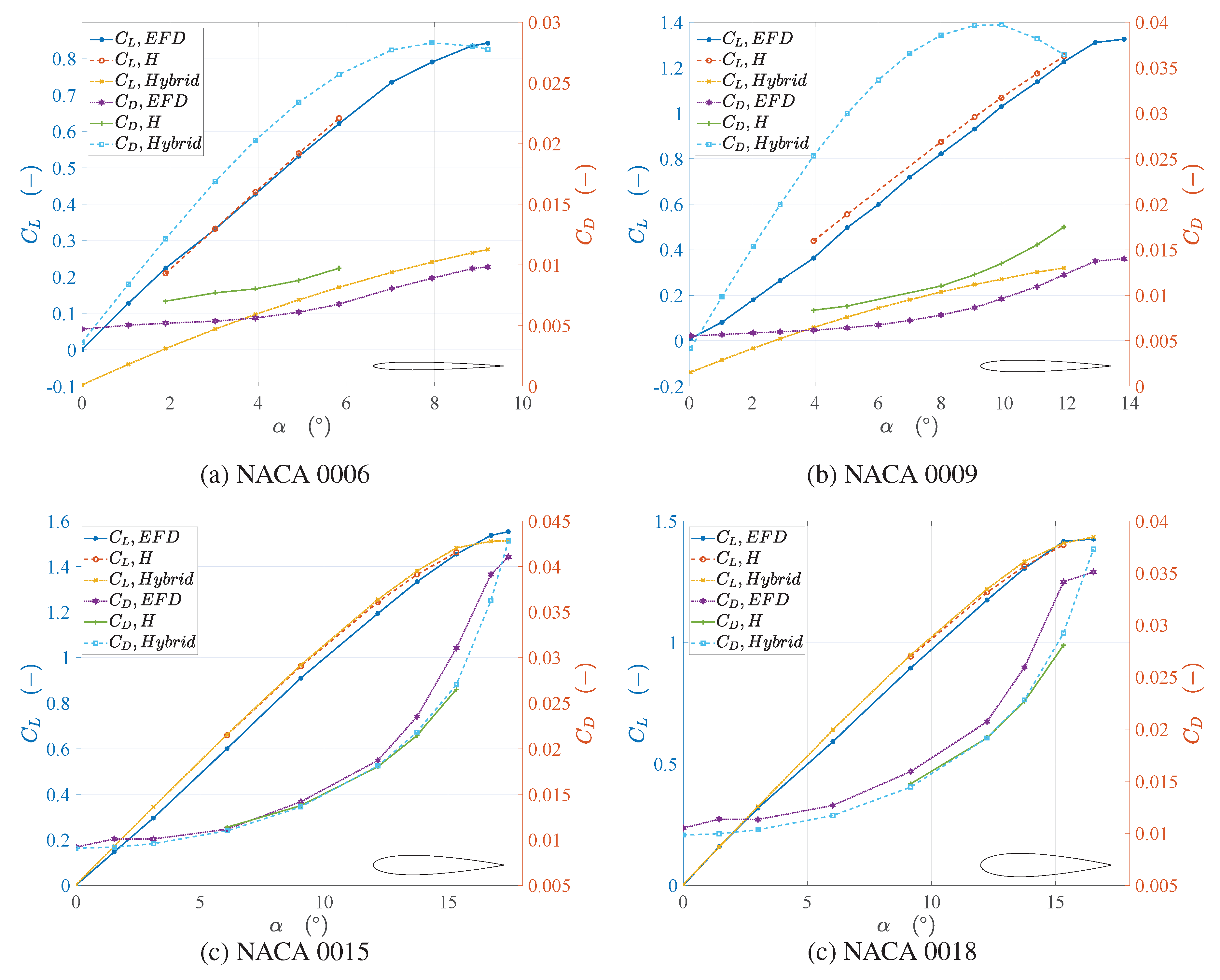
Figure 20.
Comparison of results of H and Hybrid mesh with experimental benchmark data adopted from [
39,
40] for NACA 0006, NACA 0009, NACA 0015 and NACA 0018.
Figure 20.
Comparison of results of H and Hybrid mesh with experimental benchmark data adopted from [
39,
40] for NACA 0006, NACA 0009, NACA 0015 and NACA 0018.
Table 1.
Mesh properties studies in literature: objects, Reynolds numbers, mesh types, and domain sizes.
Table 1.
Mesh properties studies in literature: objects, Reynolds numbers, mesh types, and domain sizes.
| No. | | Settings | Object | | Mesh Type | Domain Size |
|---|
| Literature | | Tested | Selected |
|---|
| 1 | Lutton [5] | NACA 0012 | | C, O | ∖ | ∖ |
| 2 | Turnock et al. [8] | NACA 0012 | | ∖ | ∖ | Outlet |
| 3 | Stuck et al. [7] | NACA 0012 | | Hybrid C,
Hybrid triangle and quadrilateral | Hybrid quad | Inlet
Outlet |
| 4 | Basha [6] | NACA 0012 | | O, C, Hybrid | Hybrid | ∖ |
| 5 | Wasberg and Reif [15] | NACA 0009,
NACA 65209 | | H | H | Inlet
Outlet |
| 6 | Tveiterås [16] | NACA 0012 | ,
| Hybrid, C | Hybrid | Outlet |
| 7 | Narsipur et al. [17] | Multi-element
airfoils | | Hybrid | Hybrid | ∖ |
| 8 | Eleni et al. [18] | NACA 0012 | | C | C | Side
Outlet |
| 9 | Van Nguyen and Ikeda [4] | NACA 0024 | | Hybrid | Hybrid | |
| 10 | Langley Research Center [19] | NACA 0012 | | C | C | Outlet |
| 11 | Nordanger et al. [20] | NACA 0012 | | Multiple patch | Multiple patch | Inlet
Outlet |
| 12 | Siddiqui et al. [21] | NACA 0015 | | C | C | Inlet
Outlet |
Table 2.
Mesh properties studies in literature: node distributions and turbulence models.
Table 2.
Mesh properties studies in literature: node distributions and turbulence models.
| No. | | Settings | Nodes Distribution | Turbulence Model |
|---|
| Literature | | Chord | Boundary Layer | Far Field |
|---|
| 1 | Lutton [5] | ∖ | ∖ | ∖ | ∖ |
| 2 | Turnock et al. [8] | 244 nodes | | 49 radial cells
99 wake cells | k- standard and RNG |
| 3 | Stuck et al. [7] | 200 nodes | | ∖ | k- RNG |
| 4 | Basha [6] | 60 nodes | | ∖ | SA |
| 5 | Wasberg and Reif [15] | ∖ |
| ∖ | SA |
| 6 | Tveiterås [16] | 340 nodes |
| ∖ | Transition SST |
| 7 | Narsipur et al. [17] | ∖ | | ∖ | k- SST |
| 8 | Eleni et al. [18] | ∖ |
| ∖ | k- SST |
| 9 | Van Nguyen and Ikeda [4] | ∖ | | ∖ | k- SST |
| 10 | Langley Research Center [19] | ∖ | ∖ | ∖ | ∖ |
| 11 | Nordanger et al. [20] | 127 nodes | | ∖ | SA |
| 12 | Siddiqui et al. [21] | ∖ | ∖ | ∖ | k- SST |
Table 3.
Numerical settings for RANS simulations with ANSYS.
Table 3.
Numerical settings for RANS simulations with ANSYS.
| Property | Setting |
|---|
| Turbulence model | k- SST |
| Pressure-velocity coupling | Coupled |
| Gradient | Least squares cell based |
| Pressure | Second order |
| Momentum | Second order upwind |
| Turbulent kinetic energy | Second order upwind |
| Specific dissipation rate | Second order upwind |
Table 4.
Comparison of results of hydrodynamic coefficients under different
with that of experimental benchmark data adopted from [
25] in relative differences.
Table 4.
Comparison of results of hydrodynamic coefficients under different
with that of experimental benchmark data adopted from [
25] in relative differences.
| Re | | | | | | | | | |
|---|
| 3.94 × 10 | 32.26 | 3.33 | 49.48 | 1.69 | 24.03 | −0.67 | 41.61 | −1.99 | 39.59 |
| 5.97 × 10 | 25.67 | 1.97 | 17.53 | 1.29 | 44.17 | −1.84 | 50.87 | −3.28 | 44.76 |
| 6.00 × 10 | 25.57 | 2.01 | 17.36 | 1.32 | 43.61 | −1.64 | 49.30 | −2.91 | 42.49 |
| 8.86 × 10 | 22.10 | 1.73 | 20.07 | 0.09 | 26.34 | −2.32 | 51.85 | −3.33 | 49.86 |
| 1.19 × 10 | 38.37 | −0.47 | 17.54 | 0.00 | 25.81 | −1.57 | 41.30 | −3.24 | 32.23 |
| 1.89 × 10 | 47.95 | 1.13 | 5.67 | −0.88 | 9.18 | −1.51 | 25.84 | −1.99 | 19.82 |
Table 5.
Comparison of results of C-mesh based on various domain sizes with that of experimental benchmark data adopted from [
25] in relative differences.
Table 5.
Comparison of results of C-mesh based on various domain sizes with that of experimental benchmark data adopted from [
25] in relative differences.
| NOC | | | | | | | |
|---|
| 160,293 | ∖ | ∖ | ∖ | ∖ | ∖ | | ∖ |
| 203,144 | −1.75 | 68.46 | −2.57 | 55.19 | 2.16 | | 61.82 |
| 251,065 | −1.46 | 65.74 | −21.04 | ∖ | ∖ | | ∖ |
| 423,225 | −2.10 | 71.32 | −3.28 | 59.88 | 2.69 | | 65.60 |
| 524,605 | −1.65 | 67.15 | −2.38 | 53.52 | 2.01 | | 60.33 |
| 160,293 | ∖ | ∖ | ∖ | ∖ | ∖ | | ∖ |
| 203,144 | ∖ | ∖ | −2.60 | 43.80 | ∖ | | ∖ |
| 251,065 | −1.31 | 50.88 | ∖ | ∖ | ∖ | | ∖ |
| 423,225 | −1.96 | 56.69 | ∖ | ∖ | ∖ | | ∖ |
| 524,605 | −1.50 | 52.33 | −2.40 | 42.50 | 1.95 | | 47.41 |
| 160,293 | ∖ | ∖ | ∖ | ∖ | ∖ | | ∖ |
| 203,144 | −1.45 | 47.99 | −2.49 | 39.87 | 1.97 | | 43.93 |
| 251,065 | −1.19 | 44.95 | −1.87 | 34.19 | 1.53 | | 39.57 |
| 423,225 | −1.83 | 50.77 | −3.27 | 44.66 | 42.55 | | 47.71 |
| 524,605 | −1.37 | 46.32 | −2.33 | 37.85 | 1.85 | | 42.08 |
| 160,293 | −0.83 | 41.54 | −1.28 | 30.84 | 1.06 | | 36.19 |
| 203,144 | −1.35 | 45.53 | −2.40 | 37.90 | 1.87 | | 41.72 |
| 251,065 | ∖ | ∖ | ∖ | ∖ | ∖ | | ∖ |
| 423,225 | −1.75 | 48.12 | −3.22 | 42.64 | 2.49 | | 45.38 |
| 524,605 | −1.29 | 43.63 | −2.28 | 35.76 | 1.78 | | 39.70 |
| 160,293 | −0.92 | 42.50 | ∖ | ∖ | ∖ | | ∖ |
| 203,144 | −1.33 | 44.90 | −2.37 | 37.43 | 1.85 | | 41.16 |
| 251,065 | −1.06 | 41.43 | −1.85 | 32.64 | 1.45 | | 37.03 |
| 423,225 | −1.71 | 46.89 | ∖ | ∖ | ∖ | | ∖ |
| 524,605 | −1.24 | 42.38 | −2.25 | 34.79 | 1.75 | | 38.59 |
Table 6.
Uncertainty estimations for 4 cases (, NOC = 203,144, 251,065, 423,225, 524,605, ) based on mesh dependency.
Table 6.
Uncertainty estimations for 4 cases (, NOC = 203,144, 251,065, 423,225, 524,605, ) based on mesh dependency.
| Solution | | | |
|---|
| p | | | p | | | p | | |
|---|
| 2.00 | 10.02 | 2.49 | 2.00 | 0.21 | 39.87 | 2.00 | 0.12 | 2.13 |
| 16.18 | 1.87 | 0.54 | 34.19 | 0.12 | 0.81 |
| 17.73 | 3.27 | 0.62 | 44.66 | 0.21 | 6.39 |
| 11.57 | 2.33 | 0.37 | 37.85 | 0.09 | 1.91 |
Table 7.
Comparison of results of C-mesh based on various chord-wise spacings with that of experimental benchmark data adopted from [
25] in relative differences with 670 nodes in chord-wise direction for reference setting.
Table 7.
Comparison of results of C-mesh based on various chord-wise spacings with that of experimental benchmark data adopted from [
25] in relative differences with 670 nodes in chord-wise direction for reference setting.
| NOC | | | | | | | | | | | | | | | |
|---|
| −2 | 169,860 | 1.85 | 18.10 | −60.52 | 1.02 | 47.98 | −22.60 | ∖ | ∖ | ∖ | ∖ | ∖ | ∖ | ∖ | ∖ | ∖ |
| −1 | 203,534 | 1.98 | 17.39 | −62.91 | 1.37 | 43.79 | −30.17 | −1.28 | 46.15 | 6.94 | −2.10 | 36.68 | 0.52 | 1.68 | 36.00 | 25.13 |
| 0 | 251,065 | 1.99 | 17.36 | −62.48 | 1.42 | 42.89 | −30.23 | ∖ | ∖ | ∖ | ∖ | ∖ | ∖ | ∖ | ∖ | ∖ |
| 1 | 318,413 | 1.98 | 17.47 | −61.99 | 1.28 | 44.17 | −26.44 | −1.81 | 50.89 | 13.49 | ∖ | ∖ | ∖ | ∖ | ∖ | ∖ |
| 2 | 413,475 | 2.01 | 17.36 | −62.58 | 1.32 | 43.61 | −27.09 | −1.64 | 49.30 | 11.47 | −2.91 | 42.49 | 4.26 | 1.97 | 38.19 | 26.35 |
| 3 | 548,022 | 2.03 | 17.15 | −63.17 | 1.44 | 42.09 | −29.86 | −1.05 | 43.73 | 4.52 | −1.76 | 34.33 | −1.74 | 1.57 | 34.32 | 24.82 |
| 4 | 738,295 | 2.03 | 17.15 | −62.90 | 1.42 | 42.16 | −28.96 | −1.12 | 44.26 | 5.42 | −1.88 | 35.22 | −1.12 | 1.61 | 34.70 | 24.60 |
| 5 | 1,007,091 | 2.02 | 17.15 | −62.63 | 1.39 | 42.23 | −28.06 | −1.18 | 44.79 | 6.31 | −1.56 | 34.66 | −0.84 | 1.54 | 34.71 | 24.46 |
Table 8.
Uncertainty estimations for C-mesh (, ) with varying chord-wise spacings based on mesh dependency.
Table 8.
Uncertainty estimations for C-mesh (, ) with varying chord-wise spacings based on mesh dependency.
| Solution | | | |
|---|
| p | | | p | | | p | | |
|---|
| 2.00 | 2.02 | 2.91 | 1.04 | 1.28 | 42.49 | 1.23 | 0.70 | 4.26 |
| 0.46 | 1.76 | 1.11 | 34.32 | 0.59 | 1.74 |
| 0.06 | 1.88 | 0.72 | 35.22 | 0.37 | 1.11 |
| 0.04 | 1.56 | 0.67 | 34.65 | 0.34 | 0.84 |
Table 9.
Comparison of results of H-mesh based on various chord-wise spacings with that of experimental benchmark data adopted from [
25] in relative differences with 386 nodes in chord-wise direction for reference setting.
Table 9.
Comparison of results of H-mesh based on various chord-wise spacings with that of experimental benchmark data adopted from [
25] in relative differences with 386 nodes in chord-wise direction for reference setting.
| NOC | | | | | | | | | | | | | | | |
|---|
| −2 | 178,209 | 2.53 | 18.68 | −83.92 | 1.08 | 61.15 | −34.30 | −3.47 | 84.99 | 23.30 | −6.28 | 81.61 | 13.11 | 3.34 | 61.61 | 38.66 |
| −1 | 208,245 | 2.61 | 17.19 | −83.64 | 1.48 | 50.20 | −39.06 | −2.55 | 64.66 | 19.18 | −4.60 | 60.33 | 10.91 | 2.81 | 48.09 | 38.20 |
| 0 | 255,852 | 2.73 | 17.41 | −85.96 | 1.82 | 45.53 | −45.29 | −1.45 | 51.54 | 8.66 | ∖ | ∖ | ∖ | ∖ | ∖ | ∖ |
| 1 | 333,306 | 2.84 | 17.90 | −88.34 | 1.97 | 43.93 | −48.35 | −1.05 | 47.09 | 4.81 | −2.09 | 37.97 | 2.96 | 1.99 | 36.72 | 36.11 |
| 2 | 462,288 | 2.84 | 17.75 | −87.83 | 2.05 | 42.18 | −49.32 | −0.67 | 41.65 | 1.45 | −1.30 | 30.54 | −0.37 | 1.72 | 33.03 | 34.74 |
| 3 | 683,862 | 2.87 | 17.24 | −87.77 | 2.08 | 41.06 | −49.42 | −0.64 | 40.21 | 1.63 | −1.28 | 29.36 | −0.09 | 1.72 | 31.97 | 34.73 |
| 4 | 1,079,760 | 2.89 | 17.06 | −88.12 | 2.13 | 40.32 | −50.54 | −0.42 | 37.89 | −1.11 | −0.85 | 26.08 | −2.60 | 1.57 | 30.34 | 35.59 |
Table 10.
Uncertainty estimations for H-mesh (, ) with varying chord-wise spacings based on mesh dependency.
Table 10.
Uncertainty estimations for H-mesh (, ) with varying chord-wise spacings based on mesh dependency.
| Solution | | | |
|---|
| p | | | p | | | p | | |
|---|
| 2.00 | 2.20 | 2.08 | 1.12 | 0.42 | 37.96 | 0.95 | 0.21 | 2.96 |
| 0.80 | 1.30 | 0.31 | 30.54 | 0.16 | 0.37 |
| 0.07 | 1.28 | 0.21 | 29.35 | 0.31 | 0.09 |
| 0.08 | 0.85 | 0.14 | 26.08 | 0.10 | 2.60 |
Table 11.
Comparison of results of O-mesh based on various chord-wise spacings to that of experimental benchmark data adopted from [
25] in relative differences with 296 nodes in chord-wise direction for reference setting.
Table 11.
Comparison of results of O-mesh based on various chord-wise spacings to that of experimental benchmark data adopted from [
25] in relative differences with 296 nodes in chord-wise direction for reference setting.
| NOC | | | | | | | | | | | | | | | |
|---|
| −2 | 116,012 | 7.66 | −0.45 | −87.30 | 25.07 | 73.38 | 16.88 | −54.32 | 1016.56 | −430.26 | −76.12 | 597.97 | −111.56 | 40.79 | 422.09 | 161.50 |
| −1 | 163,852 | 3.48 | 15.45 | −77.29 | 22.23 | 100.94 | 2.36 | −2.78 | 70.68 | 4.52 | −48.31 | 540.63 | −67.68 | 19.20 | 181.93 | 37.96 |
| 0 | 193,752 | −0.39 | 28.12 | −82.61 | 20.05 | 132.55 | 3.36 | −3.35 | 84.92 | 5.53 | −3.99 | 66.75 | −3.11 | 6.95 | 78.08 | 23.65 |
| 1 | 331,292 | −1.24 | 34.48 | −96.77 | 19.16 | 142.69 | −8.57 | −3.80 | 106.31 | −6.21 | −5.00 | 96.24 | −9.14 | 7.30 | 94.93 | 30.17 |
| 2 | 472,800 | −4.00 | 44.66 | −87.64 | 17.65 | 163.98 | −11.24 | −3.90 | 110.78 | −11.54 | −4.52 | 90.11 | −11.43 | 7.52 | 102.38 | 30.46 |
| 3 | 666,770 | ∖ | ∖ | ∖ | 17.96 | 156.92 | −6.51 | −4.74 | 124.83 | −16.92 | −52.91 | 842.17 | −653.75 | ∖ | ∖ | ∖ |
| 4 | 944,840 | −7.22 | 48.92 | −111.48 | ∖ | ∖ | ∖ | ∖ | ∖ | ∖ | −8.03 | 91.73 | 17.80 | ∖ | ∖ | ∖ |
Table 12.
Comparison of results of Hybrid-mesh based on various chord-wise spacings with that of experimental benchmark data adopted from [
25] in relative differences.
Table 12.
Comparison of results of Hybrid-mesh based on various chord-wise spacings with that of experimental benchmark data adopted from [
25] in relative differences.
| NOC | | | | | | | | | | | | | | | |
|---|
| 2.23 | 165,801 | 3.89 | 26.16 | −139.77 | 2.93 | 58.92 | −102.81 | −0.45 | 66.54 | −27.97 | −1.88 | 56.56 | −17.50 | 2.29 | 52.05 | 72.01 |
| 1.12 | 220,230 | 2.81 | 24.61 | −98.77 | 1.97 | 56.27 | −65.66 | −0.28 | 57.21 | −19.72 | −0.39 | 43.43 | −20.39 | 1.36 | 45.38 | 51.13 |
| 7.88 | 265,546 | 3.15 | 23.68 | −111.24 | 2.33 | 53.73 | −77.53 | −0.26 | 55.59 | −20.22 | −1.03 | 42.59 | −12.24 | 1.69 | 43.90 | 55.31 |
| 5.88 | 314,070 | 3.11 | 23.18 | −108.70 | 2.23 | 52.39 | −71.74 | −0.60 | 55.97 | −13.90 | −0.88 | 42.25 | −13.51 | 1.71 | 43.45 | 51.96 |
| 374,853 | 2.93 | 23.23 | −102.73 | 2.09 | 53.57 | −66.59 | −0.64 | 55.73 | −12.36 | −1.02 | 41.83 | −12.42 | 1.67 | 43.59 | 48.53 |
| 3.15 | 476,662 | 2.89 | 22.13 | −100.24 | 2.14 | 52.34 | −66.90 | −0.60 | 54.14 | −11.16 | −1.35 | 42.18 | −8.66 | 1.74 | 42.70 | 46.74 |
| 2.23 | 620,995 | 2.73 | 22.04 | −94.71 | 1.84 | 51.30 | −57.25 | −0.98 | 54.76 | −4.10 | −1.38 | 41.61 | −6.55 | 1.73 | 42.42 | 40.66 |
Table 13.
Uncertainty estimations for Hybrid-mesh (, , ) with varying chord-wise spacings based on mesh dependency.
Table 13.
Uncertainty estimations for Hybrid-mesh (, , ) with varying chord-wise spacings based on mesh dependency.
| Solution | | | |
|---|
| p | | | p | | | p | | |
|---|
| 2.00 | 8.08 | 0.88 | 1.21 | 0.13 | 42.24 | 2.00 | 0.15 | 13.50 |
| 6.58 | 1.02 | 0.12 | 41.83 | 0.06 | 12.42 |
| 5.58 | 1.35 | 0.12 | 42.18 | 0.03 | 8.66 |
| 5.96 | 1.38 | 0.08 | 41.60 | 0.004 | 6.54 |
Table 14.
Comparison of results of C-mesh based on various layer-wise growth rates with that of experimental benchmark data adopted from [
25] in relative differences.
Table 14.
Comparison of results of C-mesh based on various layer-wise growth rates with that of experimental benchmark data adopted from [
25] in relative differences.
| r | NOC | | | | | | | | | | | | | | | |
|---|
| 1.20 | 548,022 | 1.96 | 17.06 | −63.80 | 1.31 | 43.17 | −28.81 | −1.17 | 46.09 | 4.41 | −1.79 | 35.84 | −2.75 | 1.56 | 35.54 | 24.94 |
| 1.15 | 548,022 | ∖ | ∖ | ∖ | ∖ | ∖ | ∖ | ∖ | ∖ | ∖ | ∖ | ∖ | ∖ | ∖ | ∖ | ∖ |
| 1.10 | 548,022 | 2.03 | 17.17 | −63.06 | 1.42 | 42.31 | −29.35 | −1.17 | 44.87 | 5.98 | −2.01 | 35.40 | −0.40 | 1.66 | 34.94 | 24.70 |
| 1.05 | 548,022 | 2.03 | 17.16 | −62.98 | 1.42 | 42.31 | −29.26 | −1.18 | 44.88 | 6.15 | −2.02 | 35.42 | −0.30 | 1.66 | 34.94 | 24.67 |
| 1.03 | 548,022 | 2.03 | 17.16 | −63.19 | 1.43 | 42.29 | −29.67 | −1.15 | 44.80 | 5.60 | −1.95 | 35.21 | −0.81 | 1.64 | 34.86 | 24.82 |
Table 15.
Comparison of results of H-mesh based on various layer-wise growth rates that of experimental benchmark data adopted from [
25] in relative differences.
Table 15.
Comparison of results of H-mesh based on various layer-wise growth rates that of experimental benchmark data adopted from [
25] in relative differences.
| r | NOC | | | | | | | | | | | | | | | |
|---|
| 1.20 | 46,288 | 2.86 | 16.54 | −87.45 | 2.05 | 41.22 | −48.90 | −0.72 | 41.52 | 2.02 | −1.38 | 30.81 | −0.10 | 1.75 | 32.52 | 34.62 |
| 1.15 | 46,288 | 2.87 | 17.12 | −87.99 | 2.08 | 41.55 | −49.74 | −0.61 | 41.14 | 0.50 | −1.17 | 29.96 | −1.48 | 1.68 | 32.44 | 34.93 |
| 1.10 | 46,288 | 2.84 | 17.75 | −87.82 | 2.05 | 42.20 | −49.30 | −0.67 | 41.66 | 1.46 | −1.30 | 30.55 | −0.37 | 1.72 | 33.04 | 34.74 |
| 1.05 | 46,288 | 2.86 | 17.52 | −87.96 | 2.07 | 41.74 | −49.57 | −0.63 | 41.04 | 0.94 | −1.23 | 29.92 | −0.78 | 1.70 | 32.55 | 34.81 |
| 1.03 | 46,288 | 2.87 | 17.40 | −88.05 | 2.08 | 41.60 | −49.77 | −0.60 | 40.87 | 0.51 | −1.18 | 29.74 | −1.18 | 1.68 | 32.40 | 34.88 |
Table 16.
Comparison of results of Hybrid-mesh based on various layer-wise growth rates with that of experimental benchmark data adopted from [
25] in relative differences.
Table 16.
Comparison of results of Hybrid-mesh based on various layer-wise growth rates with that of experimental benchmark data adopted from [
25] in relative differences.
| r | NOC | | | | | | | | | | | | | | | |
|---|
| 1.20 | 607,987 | 2.30 | 21.80 | −81.67 | 1.23 | 50.70 | −36.72 | −1.64 | 54.72 | 7.37 | −2.14 | 44.18 | −2.79 | 1.83 | 42.85 | 32.14 |
| 1.15 | 611,491 | 2.24 | 22.13 | −80.52 | 1.36 | 51.11 | −41.85 | −1.16 | 54.54 | −1.17 | −1.43 | 41.82 | −6.33 | 1.55 | 42.40 | 32.47 |
| 1.10 | 620,995 | 2.73 | 22.03 | −94.78 | 1.84 | 51.32 | −57.42 | −0.98 | 54.76 | −4.09 | −1.87 | 43.50 | −4.28 | 1.86 | 42.90 | 40.14 |
| 1.05 | 652,233 | 2.87 | 17.74 | −98.81 | 1.78 | 48.03 | −54.62 | −1.24 | 54.52 | −0.37 | −1.69 | 41.02 | −5.83 | 1.89 | 40.33 | 39.91 |
| 1.03 | 660,281 | 3.37 | 6.31 | −109.96 | 2.16 | 38.29 | −63.27 | −1.00 | 50.00 | −3.25 | ∖ | ∖ | ∖ | ∖ | ∖ | ∖ |
Table 17.
Comparison of results of C-mesh based on various radial nodes with that of experimental benchmark data adopted from [
25] in relative differences with 150 nodes in radial directions for reference setting.
Table 17.
Comparison of results of C-mesh based on various radial nodes with that of experimental benchmark data adopted from [
25] in relative differences with 150 nodes in radial directions for reference setting.
| NOC | | | | | | | | | | | | | | | |
|---|
| −2 | 272,172 | 1.89 | 17.08 | −63.18 | 1.16 | 46.20 | −19.87 | −1.27 | 47.33 | 5.08 | −1.90 | 37.84 | −2.64 | 1.55 | 37.11 | 22.69 |
| −1 | 386,190 | 2.02 | 17.17 | −64.08 | 1.41 | 42.79 | −30.40 | −1.09 | 45.27 | 3.84 | −1.75 | 35.82 | −2.59 | 1.57 | 35.26 | 25.23 |
| 0 | 548,022 | 2.03 | 17.17 | −63.06 | 1.42 | 42.31 | −29.35 | −1.17 | 44.86 | 5.98 | −2.01 | 36.06 | −0.40 | 1.66 | 35.10 | 24.70 |
| 1 | 776,058 | 2.03 | 17.17 | −63.06 | 1.42 | 42.31 | −29.35 | −1.17 | 44.86 | 5.98 | −2.01 | 36.06 | −0.40 | 1.66 | 35.10 | 24.70 |
| 2 | 1,099,722 | ∖ | ∖ | ∖ | ∖ | ∖ | ∖ | ∖ | ∖ | ∖ | ∖ | ∖ | ∖ | ∖ | ∖ | ∖ |
| 3 | 1,555,794 | 2.04 | 17.12 | −63.04 | 1.43 | 42.15 | −29.31 | −1.17 | 44.64 | 6.04 | −2.00 | 35.88 | −0.36 | 1.66 | 34.95 | 24.69 |
| 4 | 2,203,122 | 2.04 | 17.10 | −63.02 | 1.44 | 42.08 | −29.29 | −1.16 | 44.54 | 6.06 | −2.00 | 35.80 | −0.34 | 1.66 | 34.88 | 24.68 |
Table 18.
Comparison of results of H-mesh based on various radial nodes to experimental benchmark data adopted from [
25] in relative differences with 150 nodes in radial directions for reference setting.
Table 18.
Comparison of results of H-mesh based on various radial nodes to experimental benchmark data adopted from [
25] in relative differences with 150 nodes in radial directions for reference setting.
| NOC | | | | | | | | | | | | | | | |
|---|
| −2 | 314,088 | 2.84 | 17.74 | −87.76 | 2.05 | 42.20 | −49.31 | −0.67 | 41.66 | 1.45 | −1.30 | 30.52 | −0.36 | 1.72 | 33.03 | 34.72 |
| −1 | 375,344 | 2.84 | 17.75 | −87.82 | 2.05 | 42.20 | −49.30 | −0.67 | 41.65 | 1.45 | −1.30 | 30.55 | −0.37 | 1.72 | 33.04 | 34.74 |
| 0 | 462,288 | 2.84 | 17.75 | −87.83 | 2.05 | 42.20 | −49.30 | −0.67 | 41.65 | 1.45 | −1.30 | 30.55 | −0.38 | 1.72 | 33.04 | 34.74 |
| 1 | 584,800 | 2.84 | 17.75 | −87.83 | 2.05 | 42.20 | −49.31 | −0.67 | 41.65 | 1.45 | −1.30 | 30.55 | −0.38 | 1.72 | 33.04 | 34.74 |
| 2 | 758,688 | ∖ | ∖ | ∖ | 2.05 | 42.19 | −49.30 | −0.67 | 41.65 | 1.45 | −1.30 | 30.54 | −0.38 | ∖ | ∖ | ∖ |
| 3 | 1,002,712 | ∖ | ∖ | ∖ | 2.05 | 42.19 | −49.31 | −0.67 | 41.64 | 1.45 | −1.30 | 30.53 | −0.37 | ∖ | ∖ | ∖ |
| 4 | 1,351,488 | ∖ | ∖ | ∖ | ∖ | ∖ | ∖ | −0.67 | 41.64 | 1.45 | −1.30 | 30.54 | −0.37 | ∖ | ∖ | ∖ |
Table 19.
Comparison of results of C-mesh based on various wake nodes with that of experimental benchmark data adopted from [
25] in relative differences with 300 nodes in wake directions for reference setting.
Table 19.
Comparison of results of C-mesh based on various wake nodes with that of experimental benchmark data adopted from [
25] in relative differences with 300 nodes in wake directions for reference setting.
| NOC | | | | | | | | | | | | | | | |
|---|
| −2 | 503,322 | 3.54 | 32.94 | −41.90 | 1.42 | 42.31 | −29.37 | −1.17 | 44.86 | 5.97 | −2.01 | 36.07 | −0.41 | 2.03 | 39.04 | 19.41 |
| −1 | 521,798 | 2.03 | 17.17 | −63.07 | 1.42 | 42.31 | −29.37 | −1.17 | 44.86 | 5.97 | −2.01 | 36.07 | −0.41 | 1.66 | 35.10 | 24.70 |
| 0 | 548,022 | 2.03 | 17.17 | −63.07 | 1.42 | 42.31 | −29.36 | −1.17 | 44.86 | 5.97 | −2.01 | 36.06 | −0.41 | 1.66 | 35.10 | 24.70 |
| 1 | 584,974 | 2.03 | 17.17 | −63.07 | 0.39 | 41.54 | −4.57 | −1.17 | 44.86 | 5.98 | −2.01 | 36.06 | −0.40 | 1.40 | 34.91 | 18.51 |
| 2 | 637,422 | 2.03 | 17.16 | −63.07 | 1.42 | 42.30 | −29.35 | −1.17 | 44.84 | 5.98 | ∖ | ∖ | ∖ | ∖ | ∖ | ∖ |
| 3 | 711,624 | 2.03 | 17.16 | −63.07 | 1.42 | 42.29 | −29.35 | −1.18 | 44.83 | 6.01 | −2.01 | 36.04 | −0.38 | 1.66 | 35.08 | 24.70 |
| 4 | 816,222 | ∖ | ∖ | ∖ | ∖ | ∖ | ∖ | ∖ | ∖ | ∖ | ∖ | ∖ | ∖ | ∖ | ∖ | ∖ |
Table 20.
Comparison of the results of H-mesh based on various wake nodes with that of experimental benchmark data adopted from [
25] in relative differences with 300 nodes in wake directions for reference setting.
Table 20.
Comparison of the results of H-mesh based on various wake nodes with that of experimental benchmark data adopted from [
25] in relative differences with 300 nodes in wake directions for reference setting.
| NOC | | | | | | | | | | | | | | | |
|---|
| −2 | 405,738 | 2.84 | 17.75 | −87.83 | 2.07 | 41.74 | −49.57 | −0.67 | 41.65 | 1.45 | −1.30 | 30.55 | −0.38 | 1.72 | 32.92 | 34.81 |
| −1 | 429,112 | 2.84 | 17.75 | −87.78 | 2.07 | 41.74 | −49.57 | −0.67 | 41.65 | 1.45 | −1.31 | 30.57 | −0.35 | 1.72 | 32.93 | 34.79 |
| 0 | 462,288 | 2.84 | 17.75 | −87.80 | 2.07 | 41.74 | −49.57 | −0.67 | 41.65 | 1.45 | −1.31 | 30.57 | −0.35 | 1.72 | 32.93 | 34.79 |
| 1 | 509,036 | 2.84 | 17.74 | −87.79 | 2.07 | 41.74 | −49.57 | −0.67 | 41.65 | 1.45 | −1.31 | 30.56 | −0.35 | 1.72 | 32.92 | 34.79 |
| 2 | 575,388 | 2.84 | 17.75 | −87.80 | 2.07 | 41.74 | −49.57 | −0.67 | 41.65 | 1.45 | −1.31 | 30.57 | −0.35 | 1.72 | 32.93 | 34.79 |
| 3 | 669,261 | ∖ | ∖ | −2296.89 | 2.07 | 41.74 | −49.57 | −0.67 | 41.63 | 1.46 | −1.31 | 30.54 | −0.33 | ∖ | ∖ | ∖ |
| 4 | 801,588 | ∖ | ∖ | −8910.58 | 2.07 | 41.74 | −49.57 | −0.67 | 41.63 | 1.47 | −1.31 | 30.54 | −0.33 | ∖ | ∖ | ∖ |
Table 21.
Comparison of the results of Hybrid-mesh based on various element sizes with that of experimental benchmark data adopted from [
25] in relative differences.
Table 21.
Comparison of the results of Hybrid-mesh based on various element sizes with that of experimental benchmark data adopted from [
25] in relative differences.
|
Element Size | NOC | | | | | | | | | | | | | | | |
|---|
| 0.17678c | 621,117 | 2.71 | 22.02 | −94.43 | 1.84 | 51.32 | −57.41 | −0.99 | 54.35 | −3.76 | −1.41 | 41.77 | −6.38 | 1.74 | 42.37 | 40.49 |
| 0.12500c | 719,043 | 2.59 | 21.88 | −90.64 | 1.80 | 51.40 | −55.08 | −0.72 | 53.35 | −6.48 | −1.10 | 40.96 | −8.89 | 1.55 | 41.90 | 40.27 |
| 0.08839c | 919,255 | 2.77 | 21.42 | −96.73 | 2.02 | 51.73 | −61.37 | −0.76 | 54.01 | −6.93 | −1.24 | 40.11 | −7.05 | 1.70 | 41.82 | 43.02 |
| 0.06250c | 1,314,763 | 2.70 | 21.71 | −93.17 | 1.88 | 51.95 | −57.74 | −0.86 | 54.26 | −5.91 | −1.16 | 42.14 | −9.81 | 1.65 | 42.51 | 41.66 |
| 0.04419c | 2,106,077 | 2.70 | 20.96 | −91.30 | 1.92 | 50.73 | −57.52 | −0.58 | 52.55 | −9.67 | −1.41 | 41.24 | −7.21 | 1.65 | 41.37 | 41.43 |
Table 22.
Uncertainty estimations for C-mesh with varying radial node distributions () based on mesh dependency.
Table 22.
Uncertainty estimations for C-mesh with varying radial node distributions () based on mesh dependency.
| Solution | | | |
|---|
| p | | | p | | | p | | |
|---|
| 0.23 | 2.87 | 1.90 | 2.00 | 0.06 | 37.84 | 0.56 | 0.33 | 2.63 |
| 2.69 | 1.75 | 0.04 | 35.81 | 0.23 | 2.58 |
| 1.77 | 2.00 | 0.02 | 36.06 | 0.18 | 0.40 |
| 1.27 | 2.00 | 0.02 | 36.06 | 0.16 | 0.40 |
Table 23.
Uncertainty estimations for H-mesh with varying radial node distributions () based on mesh dependency.
Table 23.
Uncertainty estimations for H-mesh with varying radial node distributions () based on mesh dependency.
| Solution | | | |
|---|
| p | | | p | | | p | | |
|---|
| 2.00 | 0.0002 | 1.30 | 2.00 | 0.0003 | 30.56 | 2.00 | 0.0001 | 0.38 |
| 0.0006 | 1.30 | 0.0002 | 30.55 | 0.0001 | 0.37 |
| 0.0004 | 1.30 | 0.0001 | 30.55 | 0.0001 | 0.37 |
| 0.0007 | 1.30 | 0.0001 | 30.55 | 0.0001 | 0.37 |
Table 24.
Uncertainty estimations for C-mesh with varying wake node distributions () based on mesh dependency.
Table 24.
Uncertainty estimations for C-mesh with varying wake node distributions () based on mesh dependency.
| Solution | | | |
|---|
| p | | | p | | | p | | |
|---|
| 2.00 | 0.003 | 2.00 | 2.00 | 0.001 | 36.06 | 2.00 | 0.001 | 0.42 |
| 0.002 | 2.00 | 0.001 | 36.06 | 0.001 | 0.42 |
| 0.001 | 2.00 | 0.001 | 36.06 | 0.001 | 0.42 |
| 0.001 | 2.00 | 0.001 | 36.06 | 0.001 | 0.42 |
Table 25.
Uncertainty estimations for H-mesh with varying wake node distributions () based on mesh dependency.
Table 25.
Uncertainty estimations for H-mesh with varying wake node distributions () based on mesh dependency.
| Solution | | | |
|---|
| p | | | p | | | p | | |
|---|
| 2.00 | 0.0102 | 1.30 | 2.00 | 0.0002 | 30.55 | 2.00 | 0.0006 | 0.38 |
| 0.0057 | 1.31 | 0.0006 | 30.57 | 0.0002 | 0.35 |
| 0.0032 | 1.31 | 0.0006 | 30.57 | 0.0001 | 0.35 |
| 0.0017 | 1.31 | 0.0007 | 30.56 | 0.0001 | 0.35 |
Table 26.
Uncertainty estimations for Hybrid-mesh (Element size = , , ) with varying far-field node distributions based on mesh dependency.
Table 26.
Uncertainty estimations for Hybrid-mesh (Element size = , , ) with varying far-field node distributions based on mesh dependency.
| Solution | | | |
|---|
| p | | | p | | | p | | |
|---|
| 2.00 | 0.14 | 1.41 | 2.00 | 0.16 | 41.77 | 0.86 | 0.63 | 6.38 |
| 0.17 | 1.10 | 0.15 | 40.96 | 0.61 | 8.88 |
| 0.14 | 1.24 | 0.24 | 40.11 | 0.57 | 7.04 |
| 0.12 | 1.16 | 0.20 | 42.14 | 0.43 | 9.81 |
Table 27.
Recommended mesh properties for different mesh types.
Table 27.
Recommended mesh properties for different mesh types.
| Mesh Types | C-Mesh | H-Mesh | O-Mesh | Hybrid-Mesh |
|---|
| Mesh Properties | |
|---|
| | | | |
| Domain size | | | | |
| Chord-wise spacing | 1895 nodes | 692 nodes | 658 nodes | |
| Layer-wise growth rate | 1.10 | 1.05 | ∖ | 1.10 |
| Far-field node distribution | Radial-150 nodes | Radial-150 nodes | Radial-∖ | Element size- |
| Wake-300 nodes | Wake-300 nodes | Wake-∖ |
| Number of cells | | | ∖ | |
Table 28.
Comparison of mesh types with recommended settings to that of other CFD codes adopted from [
19] in relative differences.
Table 28.
Comparison of mesh types with recommended settings to that of other CFD codes adopted from [
19] in relative differences.
| Codes | () | | |
|---|
| C-Mesh | H-Mesh | Hybrid-Mesh | C-Mesh | H-Mesh | Hybrid-Mesh |
|---|
| CFL3D | 0 | \ | \ | \ | 0.91% | 1.44% | 3.47% |
| 10 | −0.57% | −0.01% | 0.05% | 7.88% | 7.18% | 16.02% |
| 15 | −1.37% | −0.72% | −0.63% | 11.05% | 6.80% | 15.94% |
| FUN3D | 0 | \ | \ | \ | 1.03% | 1.57% | 3.60% |
| 10 | −1.13% | −0.58% | −0.53% | 6.42% | 5.72% | 14.45% |
| 15 | −1.64% | −0.99% | −0.90% | 8.31% | 4.17% | 13.09% |
| NTS | 0 | \ | \ | \ | 0.91% | 1.44% | 3.47% |
| 10 | −0.45% | 0.11% | 0.17% | 6.59% | 5.89% | 14.63% |
| 15 | −1.58% | −0.93% | −0.84% | 12.67% | 8.36% | 17.64% |
Table 29.
More profiles studied.
Table 29.
More profiles studied.
| Profile | | Reference |
|---|
| NACA 0006 | | Abbott and Doenhoff [39] |
| NACA 0009 | | Abbott and Doenhoff [39] |
| NACA 0015 | | Jacobs and Sherman [40] |
| NACA 0018 | | Jacobs and Sherman [40] |
Table 30.
Recommended mesh properties for different objective.
Table 30.
Recommended mesh properties for different objective.
| Objective | Properties | Settings |
|---|
| Accurate prediction for both and | Mesh type | H-mesh |
| Actual Reynolds number whenever possible |
| Domain size | As large as possible or at least around and after the profile |
| Chord-wise spacing | More than 692 nodes for m |
| Layer-wise growth rate | 1.05 |
| Number of radial nodes | 150 nodes |
| Number of wake nodes | 300 nodes |
| Number of mesh cells | No less than |
| Accurate only with less mesh number | Mesh type | C-mesh |
| |
| Domain size | around and after the profile |
| Chord-wise spacing | 670 nodes for m |
| Layer-wise growth rate | 1.10 |
| Number of radial nodes | 150 nodes |
| Number of wake nodes | 300 nodes |
| Number of mesh cells | About |
| Acceptable and with simple meshing strategy | Mesh type | Hybrid-mesh |
| |
| Domain size | around and after the profile |
| Chord-wise spacing | |
| Layer-wise growth rate | 1.10 |
| Element size | |
| Number of mesh cells | About |


