Analysis of the Formation Mechanism and Evolution of the Perpendicular Cavitation Vortex of Tip Leakage Flow in an Axial-Flow Pump for Off-Design Conditions

Abstract

To understand the formation mechanism and evolution process of the perpendicular cavitation vortex (PCV) of an axial flow pump for off-design conditions, turbulent cavitating flows were numerically investigated using the rotation curvature-corrected shear stress transport (SST-CC) turbulence model and the Zwart–Gerber–Belamri cavitation model. In this work, the origin and evolution of a PCV were analyzed through a high-speed photography experiment and numerical simulation. The results showed that the PCV came from a secondary tip leakage vortex (S-TLV) and was aggregated by the action of the re-entrant jet, combined with the cavitation bubbles driven by the radial flow to form the cavitation vortex (CV). With the joint action of leakage jet lifting and TLV entrainment, the PCV was reoriented and gradually became perpendicular to the chord direction. Then, the PCV and TLV collided, mixed, and entrained, which formed a strong pressure pulsation. The PCV was gradually divided into upper and lower parts. One part was combined with the residual part of the TLV and flowed to the next blade, and the other part flowed out of the impeller area along the axial direction. At the same time, the generation, evolution, and dissipation of the PCV formed high pulsation amplitudes and frequencies in the middle and rear above the blade suction.

1. Introduction

An axial flow pump has the characteristics of large flow rate, high efficiency and low head. It is widely used in water diversion, marine water jet propulsion, irrigation, nuclear power and other fields [1,2]. Due to the rotational operation of the axial flow pump impeller, there is inevitably a certain gap between the rotating blades and the fixed impeller chamber. The pressure difference between the pressure side (PS) and the suction side (SS) of the blade induces a tip leakage jet near the tip clearance. The jet starts from the PS near the blade tip, accelerates in the gap, and transforms into a tip leakage vortex (TLV) as it rolls up on the SS [3,4,5,6]. It is beneficial and important to investigate the effect of the impeller’s geometry on the vortices and understand the evolution mechanisms of the tip clearance flow and vortices [7,8,9,10,11]. You et al. [12,13] used the large eddy simulation (LES) method to study the tip clearance flow, focusing on the instability of the TLV structure. They thought that the velocity gradient produced by the tip leakage jet was the cause of turbulent kinetic energy (TKE) and vorticity. Zhang et al. [14] compared the tip leakage flow for right-angle and rounded tip geometries and found that the formation of the TLV originated from the continuous shear between the tip leakage jet and the low-velocity fluid on the suction side. The low-speed fluid, which underwent energy transportation from the shear layer, eventually evolved into the TLV structure. Michea Giuni et al. [15] studied the formation and evolution of the wingtip vortex formed on a square wingtip and a round wingtip through experiments, and they found that the square blade tip formed an unstable secondary vortex that affected the main vortex structure. The axial velocity had an important influence on the evolution of the vortex structure. Moghadam et al. [16] conducted a large eddy simulation of the flow in an axial fan, and they studied the dynamics of the clearance flow with several clearance sizes for design and non-design conditions.

Cavitation refers to a phenomenon that occurs when the local pressure is less than the vaporization pressure. The cavitation not only induces flow instability, but also has a serious impact on the performance of hydraulic machinery [17,18,19,20]. The tip leakage flow and cavitation significantly reduce the axial flow. Tip leakage flow and cavitation will aggravate the turbulent pulsation near an impeller chamber, causing obvious efficiency loss. In addition, due to the influence of the leakage vortex and cavitation, the inflow into the next blade is disturbed and noise is generated. The TLV and cavitation will adversely affect the hydraulic performance of the axial flow pump. At present, the main focus of research is on the generation and evolution mechanism of TLV, as well as the interaction between a vortex and cavitation. Dreyer [21] conducted experimental studies on the flow around the hydrofoil under different cavitation conditions, and suggested that cavitation would reduce the flow velocity near the TLV. Decaix et al. [22] conducted a numerical analysis on the NACA0009 hydrofoil and found that cavitation changed the TLV vorticity distribution and vortex core trajectory. Chen et al. [23] studied how cavitation affected the vorticity and turbulence of the TLV, using the LES method to simulate the hydrofoil clearance flow. Guo et al. [24] studied the interaction between TLV and cavitation for an axial flow propulsion pump and found that cavitation will increase the pressure pulsation amplitude and reduce the leakage flow.

Tan et al. [25] found that vortex cavitation occurred at the trailing edge of the sheet-shaped cavity near the tip of a blade, and the vortex cavitation was guided and redirected by the TLV in a direction almost perpendicular to the suction surface of the blade. The most significant vortex was defined as the perpendicular cavitation vortex (PCV). Zhang et al. [26] simulated the formation of a three-dimensional tip leakage vortex cavitation cloud and the periodic collapse of TLV-induced suction-side perpendicular cavitating vortices (SSPCV), which were consistent with the observations reported by Tan et al. Shi et al. [27] used numerical calculations combined with visualization experiments to reveal the influence of the flow rate, number of blades, and blade tip geometry on the PCV, with particular emphasis on the trajectory and dynamics of the PCV. The SSPCV were generated from the trailing edge of the cloud, resulting in the collapse of the triangular area. Shen et al. [28,29] studied the generation of SSPCV from the trailing edge of the cloud cavitation when the axial flow pump had a lower cavitation number. The evolution process of SSPCV can be divided into three stages: generation, shedding, and dissipation. As the flow rate decreases, the shedding frequency of the SSPCV increases, and the shedding cavities will block the flow path and reduce the performance of the pump.

Although these investigations have revealed gross features of the PCV structures and related flow phenomena, the formation mechanism, details of the vortex evolution, pressure pulsation, especially the vortex origin of the PCV, are still not very clear, and further analysis and research are needed.

Due to technical issues, it is difficult to experimentally measure the tip leakage flow near a tip gap very close to an end wall. Additionally, when cavitation occurs, it is difficult to obtain accurate flow information inside a cavity with experimental methods [30,31,32,33]. Numerical simulation can provide detailed and insightful information about the evolution of tip leakage vortex flow and unsteady cavitation flow based on the Reynolds averaged Navier–Stokes (RANS) equations [8,9,10,19,20,22,24,26,27,28,29,30].

It is found through visualization experiments that the PCV becomes stronger under off-design conditions [27,28,29], and this is obviously beneficial to observation and research. Therefore, the axial flow pump under the off-design working condition was selected (Q = 0.8 Q_BEP).

In this study, numerical simulations applying the modified shear stress transport (SST) k-ω and Zwart–Gerber–Belamri cavitation model were conducted to investigate cavitating turbulent flows in an axial flow pump. Firstly, the geometry, experimental device, and numerical calculation method of the axial flow pump are described. Secondly, the experiment for the high-speed photography of an axial flow pump with off-design conditions is explained. Then, through the transient analysis of the numerical calculation, the origin and the evolution of a PCV are described and analyzed in detail. Finally, the pressure pulsation formed by the PCV is explained.

2. Pump Geometry and Experimental Method

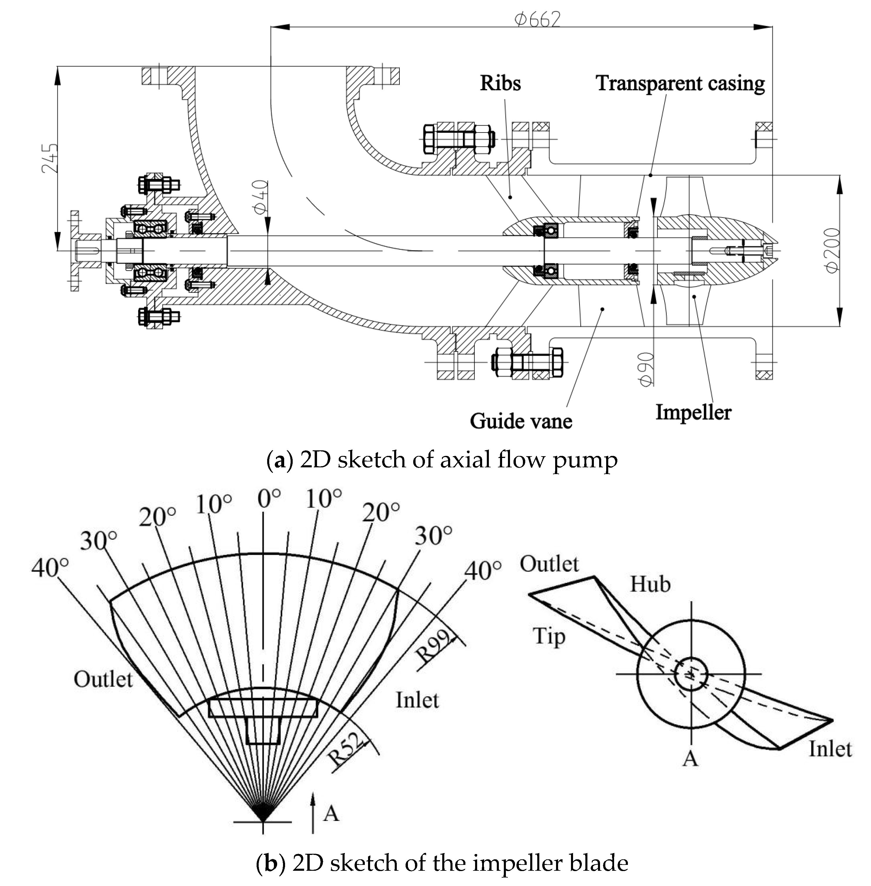
2.1. Pump Geometry

The model pump was mainly composed of three blade impellers, seven blade guide vanes, the ribs supporting the stator, and discharge elbows. The three-dimensional structure, sketches, and blade geometry of the model pump components are shown in Figure 1.

The detailed geometric parameters of the pump model are shown in

Table 1. Pump geometry and reference data.

Parameters	Value
Number of rotor blades (Zi)	3
Number of stator blades (Zd)	7
Optimum flow rate (QBEP)	0.101 m3 s−1
Chord length (c)	113.7 mm
Rotor diameter (d3)	198 mm
Hub diameter (dt)	90 mm
Inlet diameter (d1)	200 mm
Outlet diameter (d2)	250 mm
Tip clearance (τ)	1 mm
Tip velocity (Utip)	15.18 m s−1
Rotor angular velocity (Ω)	151.84 rad s−1 (1450 rpm)

.

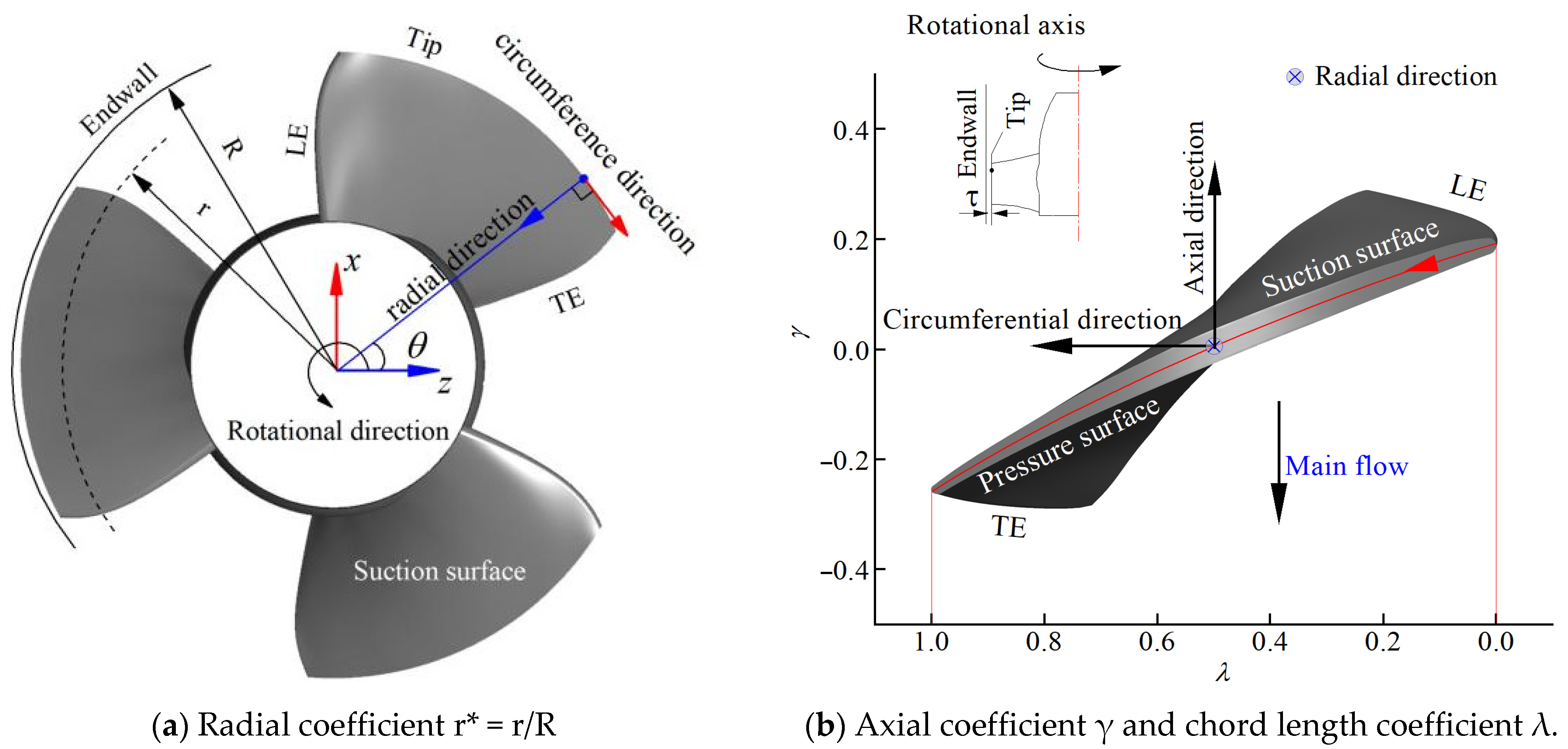
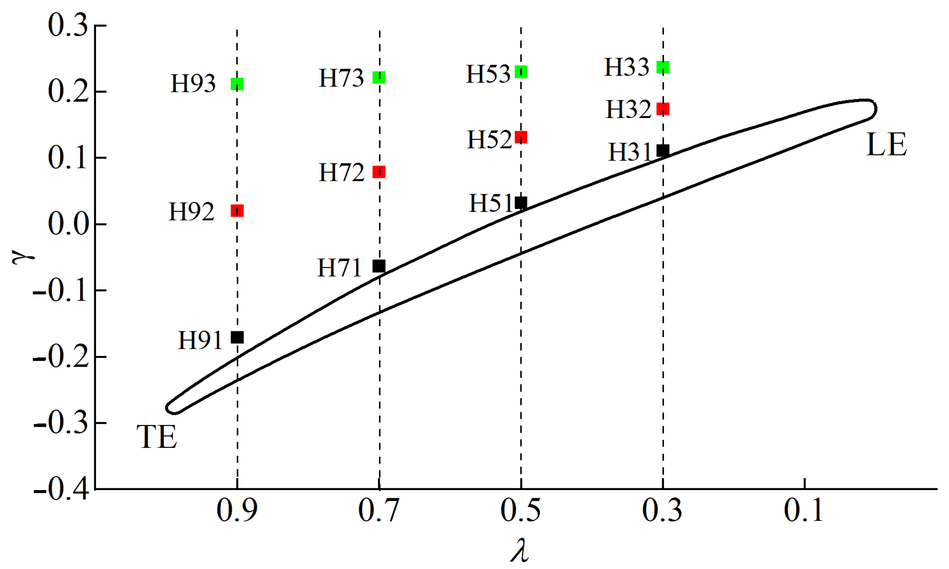
2.2. Geometric Definition of Impeller

Figure 2 shows the relevant parameters of the impeller for ease of explanation. The radial direction is shown in Figure 2a. The radial coefficient was defined as r* = r/R, where r is the radius of any point of the blade. The circumferential direction was the tangential direction corresponding to the circle of revolution, and it was perpendicular to the radial direction. The axial direction was aligned with the y-axis and the axial coefficient was defined as γ = y/R, where R is the radius of the impeller chamber, with a size of 100 mm. The main flow direction was from the pump inlet to the outlet. The blade chord coefficient was also defined λ = s/c, where s is the distance from the LE to the section of chord. The chordwise direction was from the leading edge (LE) to the tailing edge (TE).

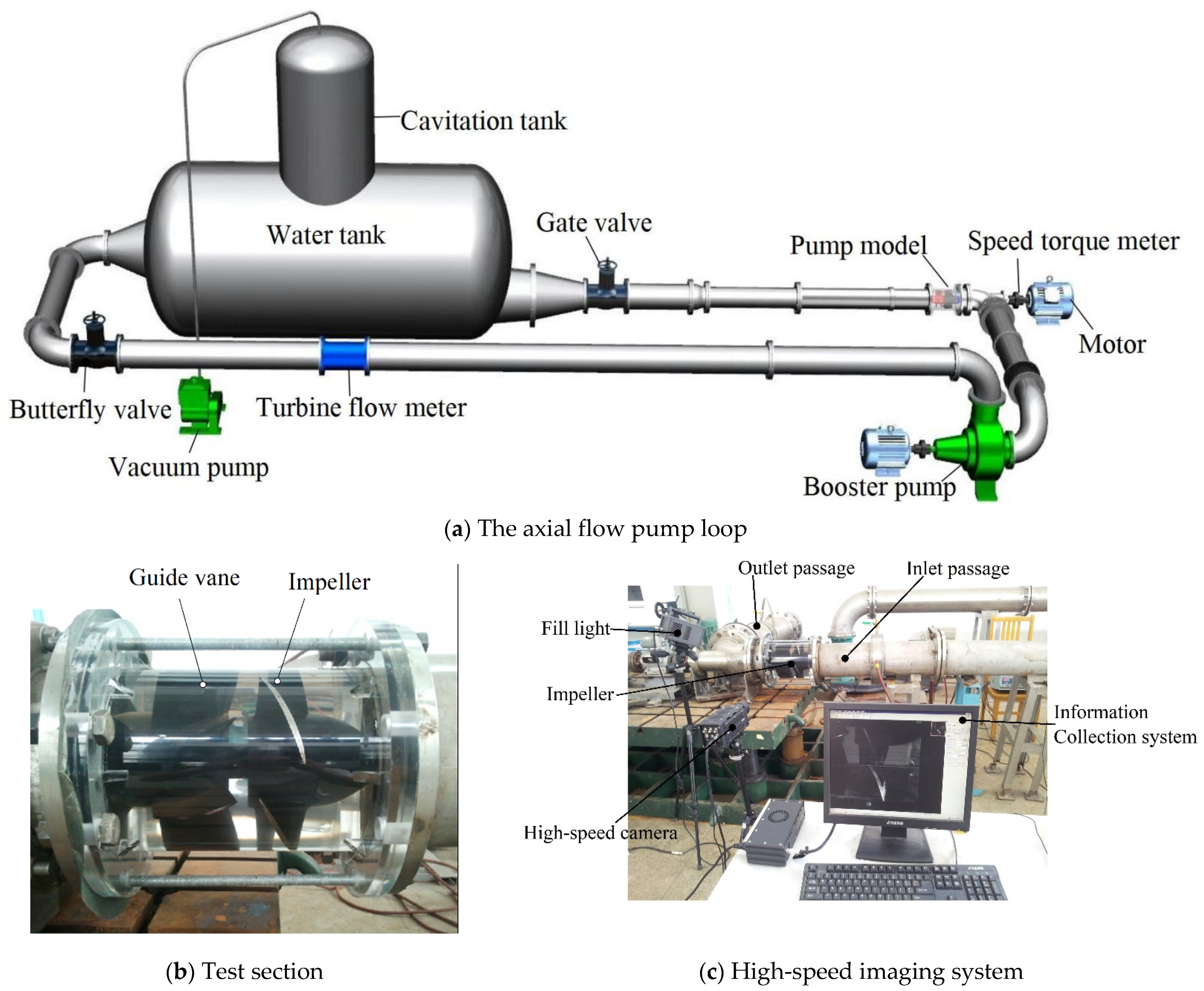
2.3. Experimental Device

Figure 3 shows the cavitation experiment and external characteristic test equipment of the axial flow pump. The test loop consisted of an axial flow pump model, a gate valve, a boosting pump, a water tank, a turbine flow meter, and a butterfly valve, as shown in Figure 3a. In order to achieve different cavitation number conditions, the cavitation tank located above the loop was connected to the vacuum pump to adjust the pressure at the inlet of the pump. The water tank had a large water storage capacity, which could keep the water temperature and flow rate relatively stable. In order to reduce the scale of inflow turbulence and improve the flow uniformity, a honeycomb wall was installed in the center of the water tank. Pressure transducers were installed in the pump inlet and outlet pipes to calculate the pump head. The speed torque meter was installed to measure the shaft speed and power. The flow rate was measured by a turbine flow meter.

In the test section, the guide vane and impeller were covered with transparent glass, as shown in Figure 3b. The images of cavitation bubbles in the area near the tip were recorded by the high-speed camera. The high-speed imaging system consisted of an information collection system, a macro lens, a high-speed camera, and fill lights, as shown in Figure 3c.

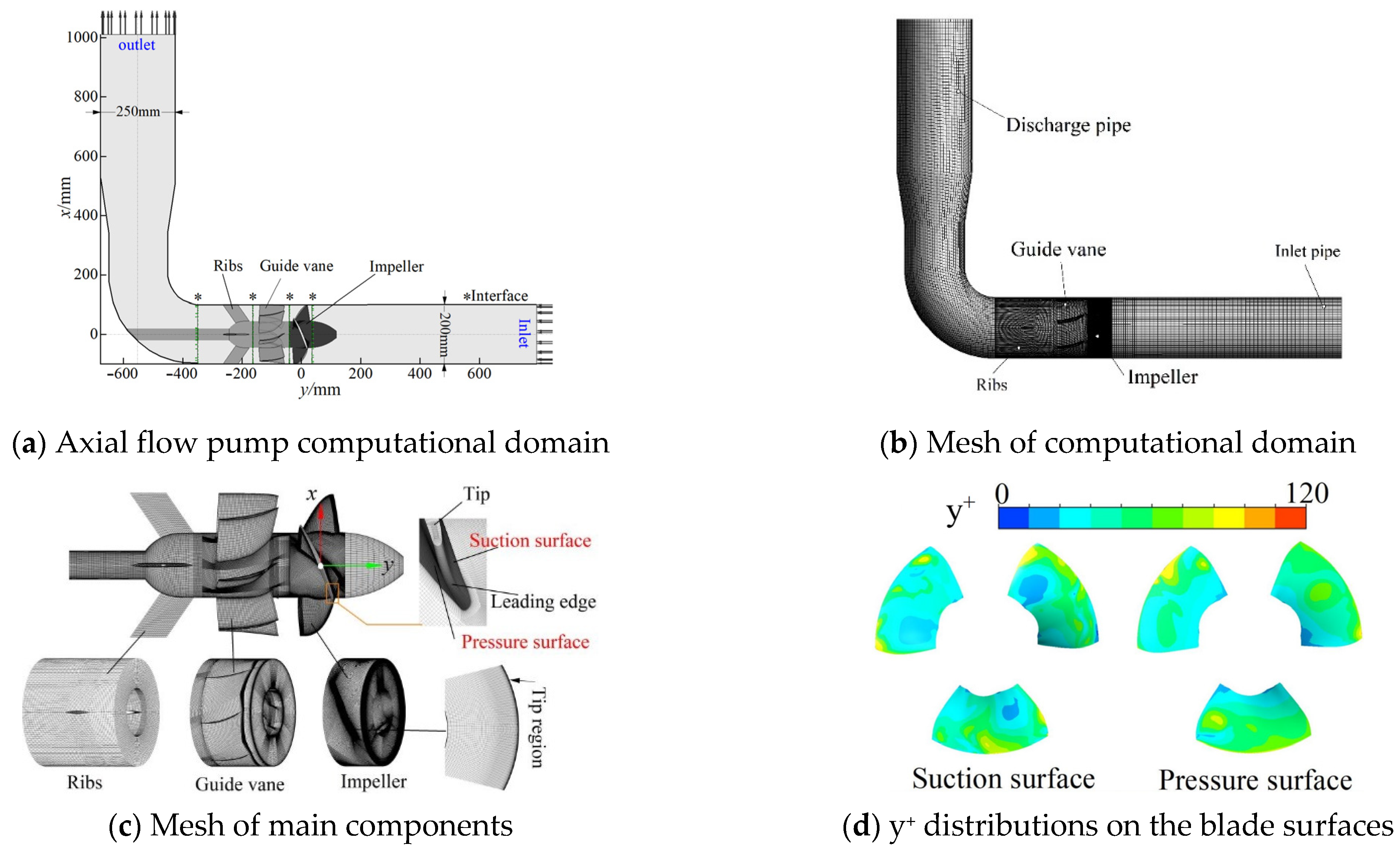
3. Calculation Method and Setting

3.1. Governing Equations, Turbulence Model, and Cavitation Model

The cavitating turbulent flows were modeled based on the homogeneous assumption, in which the multiphase flows of the liquid and vapor were considered to share the same velocity and pressure. The continuity and momentum equations for the mixture flow are expressed as follows [34]:

$$\frac{\partial \rho }{\partial \mathrm{t}}+\frac{\partial }{\partial x_j}(\rho u_j)=0$$

(1)

$$\frac{\partial }{\partial t}\left(\rho u_i\right)+\frac{\partial }{\partial x_j}\left(\rho u_i{u}_j\right)=-\frac{\partial p}{\partial x_i}+\frac{\partial }{\partial x_j}\left[\left(\mu +{\mu }_{\mathrm{t}}\right)\left(\frac{\partial u_i}{\partial x_{{}_j}}+\frac{\partial u_j}{\partial x_i}-\frac{2}{3}\frac{\partial u_k}{\partial x_k}{{\displaystyle \delta }}_{ij}\right)\right]$$

(2)

where $u_{\mathrm{i}}$ is the velocity component in the ith direction, $p$ is the pressure, and ${\mu }_T$ is the turbulent viscosity. The dynamic viscosity $\mu$ and density $\rho$ were defined as $\mu ={\alpha }_{\mathrm{v}}{\mu }_{\mathrm{v}}+(1-{\alpha }_{\mathrm{v}}){\mu }_{\mathrm{l}}$ and $\rho ={\alpha }_{\mathrm{v}}{\rho }_{\mathrm{v}}+(1-{\alpha }_{\mathrm{v}}){\rho }_{\mathrm{l}}$, respectively, where the subscripts l and v represent the liquid and vapor phases, respectively. ${\alpha }_{\mathrm{v}}$ is the vapor volume fraction.

The SST k-ω model was developed by Menter [35]. This model took into account the turbulent shear stress transport, and it could accurately predict the flow separation for an adverse pressure gradient. This eddy viscosity model was proven to be highly adaptable and feasible for tip clearance leakage flows in many examples [36,37,38]. Based on the SST k-ω equations, Smirnov and Menter proposed a modified SST model using rotational curvature correction (CC) [39,40]. Specifically, the turbulent kinetic energy production term was corrected by using a multiplier f_r. This turbulence model was called the SST-CC model, and the model could avoid the problem of the excessively fast decay of the vortex core axial velocity due to the overestimation of the eddy viscosity in the vortex. The details for the SST-CC model are available in Smirnov and Menter’s research. This model was confirmed and showed good applicability [8,39,40]. Therefore, this two-equation model was used to predict the turbulent vortex flows and cavitation.

The cavitation model used in this paper was proposed by Zwart, Gerber, and Belamri [41]. It was based on the hypothesis that all the bubbles in a system have the same size. The cavitation process is governed by the mass transfer equations for the conservation of the vapor volume fraction, which could be expressed as

$$\frac{\partial ({\rho }_{\mathrm{v}}{\alpha }_{\mathrm{v}})}{\partial t}+\frac{\partial ({\rho }_{\mathrm{v}}{\alpha }_{\mathrm{v}}{u}_j)}{\partial x_j}={\dot{m}}^{+}+{\dot{m}}^{-}$$

(3)

The source terms for the specific mass transfer rate corresponding to the vaporization ${\dot{m}}^{+}$ and condensation ${\dot{m}}^{-}$ are expressed as follows:

$${\dot{m}}^{+}=F_{\mathrm{vap}}\frac{3{\alpha }_{\mathrm{nuc}}(1-{\alpha }_{\mathrm{v}}){\rho }_{\mathrm{v}}}{R_{\mathrm{b}}}\sqrt{\frac{2}{3}\frac{p_{\mathrm{v}}-p}{{\rho }_{\mathrm{l}}}}\begin{array}{cc}& p\le p_{\mathrm{v}}\end{array}$$

(4)

$${\dot{m}}^{-}=F_{\mathrm{cond}}\frac{3{\alpha }_{\mathrm{v}}{\rho }_{\mathrm{v}}}{R_{\mathrm{b}}}\sqrt{\frac{2}{3}\frac{p-p_{\mathrm{v}}}{{\rho }_{\mathrm{l}}}}\begin{array}{cc}& p\ge p_{\mathrm{v}}\end{array}$$

(5)

where F_vap and F_cond are the empirical coefficients for the mass transfer process with the recommended values of 50 and 0.01, respectively, R_b is the typical bubble radius with a value of 1 × 10⁻⁶ m, $p_{\mathrm{v}}$ is the saturation vapor pressure, with a value of 3169 Pa, and α_nuc is the nucleation site volume fraction with a value of 5 × 10⁻⁴. These parameters were validated for the simulations of cavitating flows in pumps [26,27,28,29,30,38,42].

The commercial code ANSYS CFX 17.1 was used in this study since it is widely used in engineering applications.

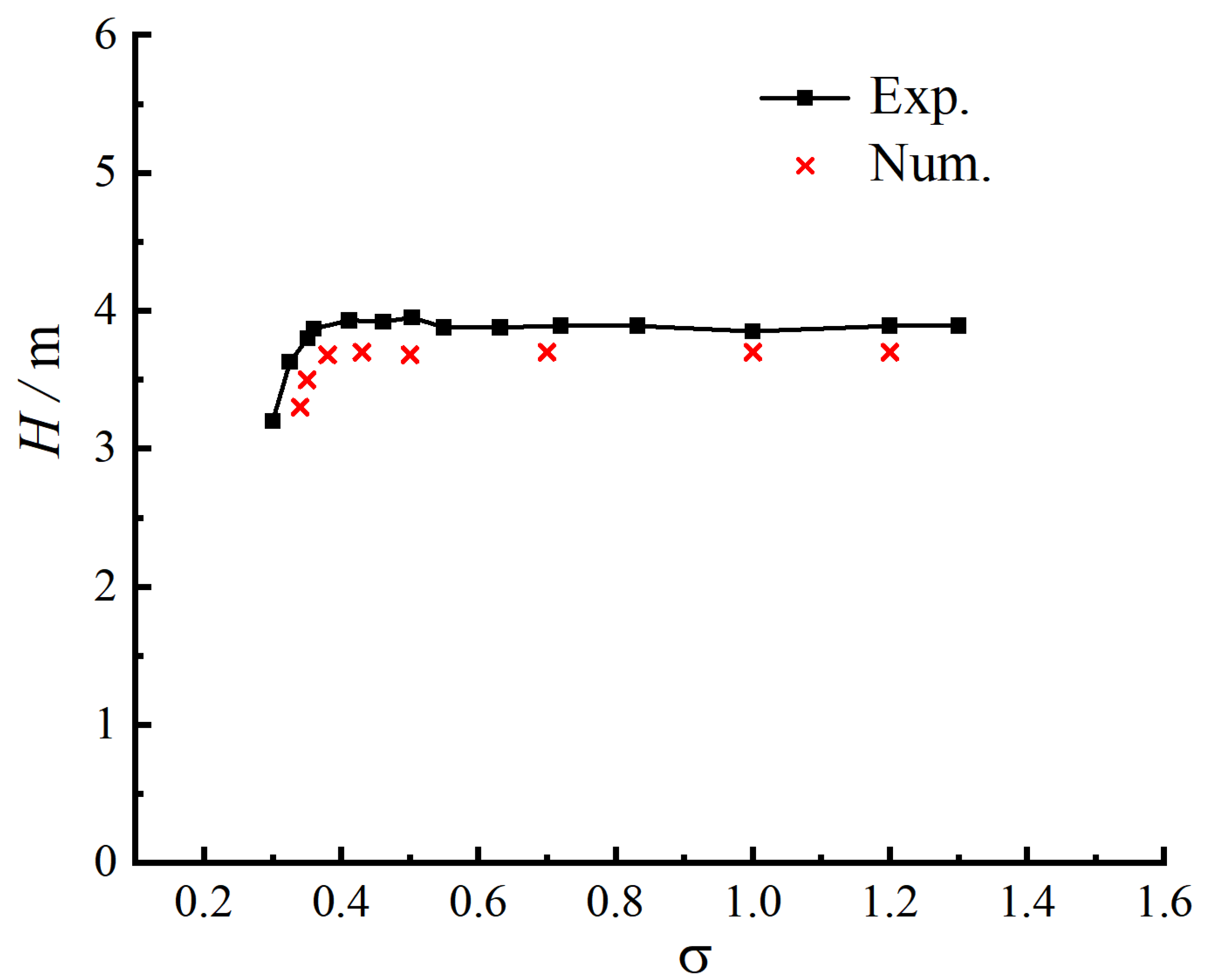
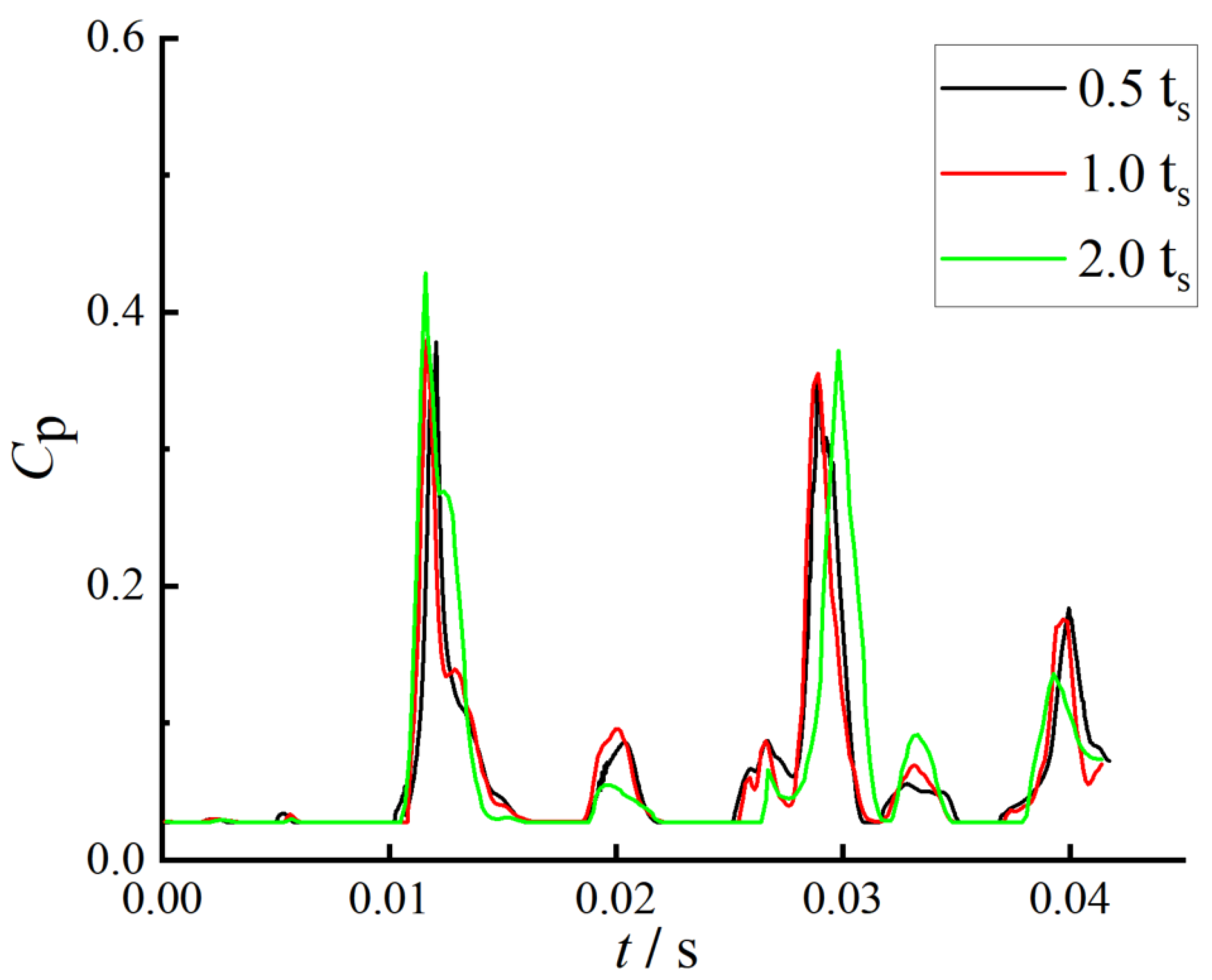
3.2. Numerical Calculation Result Verification

The mesh generation was critical for predicting the TLV and cavitation in the tip region. Thus, the arrangement of the mesh nodes in the tip region had to be appropriate to solve the large-scale tip leakage vortex and other vortices. In order to verify the applicability of the grid density to the simulation results, three groups of grids with numbers of nodes ranging from 5.42 million to 9.56 million were selected to conduct the simulation with the design conditions. The grid-independent results are presented in

Table 2. Grid-independent results.

Test Case	Mesh Nodes	Mesh Topology	Convergence Precision	Relative Head	Relative Efficiency
Case A	5,425,730	Structured	10−5	1	1
Case B	7,346,326	Structured	10−5	1.0231	1.0121
Case C	9,563,258	Structured	10−5	1.0232	1.0121

. The relative head was H_r = H/H_A, where H_A is the head of case A, and H is the calculated head. Similarly, the relative efficiency was η_r = η/η_A, where η_A is the efficiency of case A, and η is the calculated efficiency. The head H is calculated by H = (p_out−p_in)/(ρ_l g), and the efficiency η is calculated by η = gHQ(M_eΩ)⁻¹, where p_out, p_in represents the pump inlet and outlet pressure, M_e represents shaft torque and Q represents flow rate.

In order to be able to capture the small-scale vortex structure and flow details, the mesh Case C was selected, and the total number of mesh nodes was 9,563,258.

The axial flow pump computational domain is shown in Figure 4a, which consists of an inlet pipe, an impeller with three blades, ribs supporting the stator, a guide vane with seven blades, and a discharge elbow pipe. The computational domain is meshed with the hexahedral structure, as shown in Figure 4b. The mesh details of the main components such as the impeller, guide vanes and ribs are shown in Figure 4c. In order to capture the details of the tip leakage flow, the grid at the tip clearance was refined with 35 mesh nodes. The distribution of y⁺ on the blade surfaces is shown in Figure 4d. The average y⁺ values on the blade surfaces, blade tip and casing wall were 43.6, 32.8 and 16.2, respectively. This distribution indicates that the mesh nodes were suitable for the turbulence model [34].

The setting of the boundary conditions should be consistent with the experiment. In the experiment, the inlet pressure of the axial flow pump was adjusted to obtain the desired cavitation number. The outlet flow rate was adjusted to make the outlet flow rate equal to 0.8 Q_BEP, so that the axial flow pump worked under off-design conditions. The inlet was set as a total pressure condition based on the measured data in the experiment. By reducing the inlet pressure, the axial flow pump could be operated under different cavitation conditions. The cavitation number was defined as follows:

$$\sigma =2\left(p_{\mathrm{in}}-p_{\mathrm{v}}\right)/{\rho }_{\mathrm{l}}{U}_{\mathrm{tip}}{}^2$$

(6)

where $p_{\mathrm{in}}$ is the inlet pressure. The outlet was set as the mass flow rate, and the corresponding flow rate was 0.8 Q_BEP. The transient rotor–stator was used for the frame change of the impeller. All the physical surfaces of the pump were set as no-slip walls. The automatic near-wall function was used as the wall treatment method. The impeller rotational speed was 1450 r/min. The time required for the impeller to complete one revolution was denoted as T. The convergence accuracy was set to 1 × 10⁻⁵.

The influence of time step on the transient flow field was validated, based on three different time steps. One of the calculation time steps was set to t_s = 1/360 T (about 1.1494 × 10⁻⁴ s), and the other two time steps were set to 2 t_s and 0.5 t_s, respectively.

The pressure coefficient C_p is defined as follows:

$$C_p=p/0.5\rho U_{\mathrm{tip}}^2$$

(7)

Take a monitoring point above the blade clearance, which rotates with the impeller, and monitor the pressure coefficient under the same initial value of the three time step cases. The time histories of C_p in Figure 5 show that the curves of 0.5 t_s and 1.0 t_s are nearly the same, while there is a deviation for 2.0 t_s, especially in the turning points. Considering the calculation efficiency, the time step 1.0 t_s was adopted.

The time-averaged value of the pump head H obtained via the transient calculation was compared with that from the experiment. The applicability of the mesh and the turbulence model was verified by comparison of the numerical simulations and the external characteristics experiment. Compared with the experimental results, the calculation error induced by the limitations of the turbulence model, the homogeneous cavitation model, and so on, was acceptable, as shown in Figure 6.

4. Results and Discussion

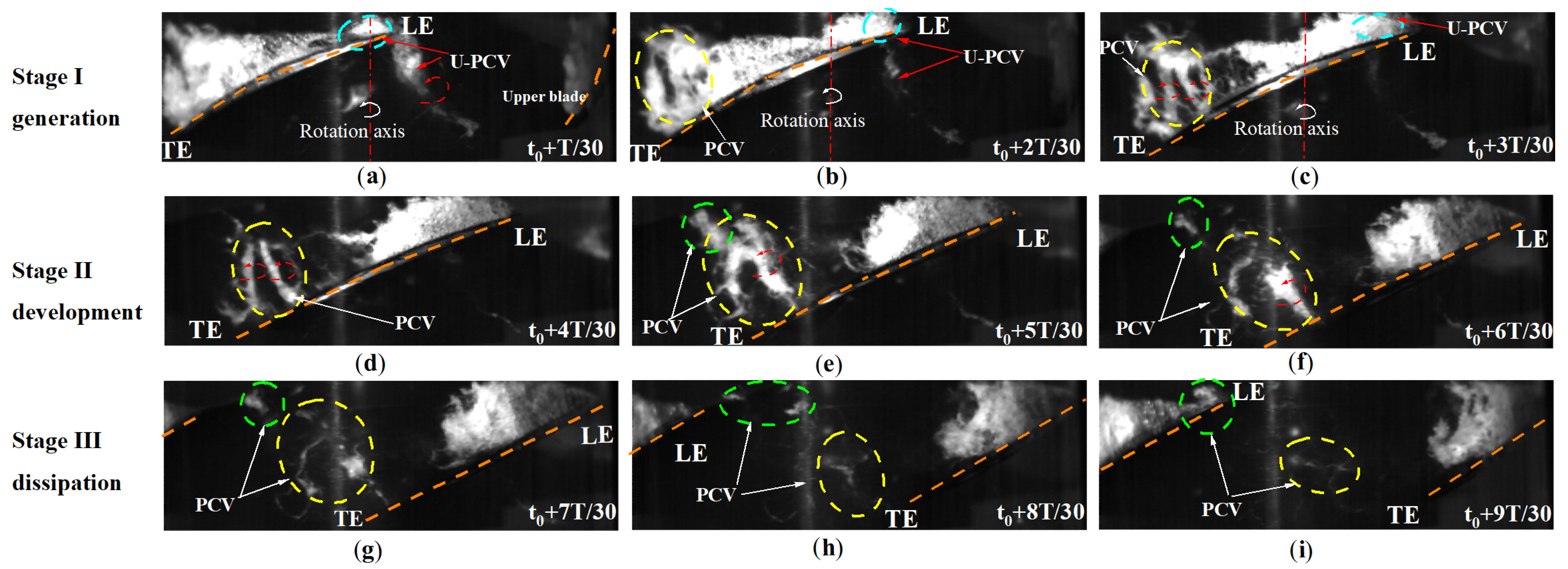
4.1. Experimental Phenomena

In the experiment, the inlet pressure of the axial flow pump was adjusted to make the cavitation number equal to 0.35, and the outlet flow was adjusted to make the outlet flow equal to 0.8 Q_BEP. Then, the axial flow pump worked under off-design conditions. After stable operation for a period of time, several groups of pictures were captured through high-speed photography, as shown in Figure 7.

When the axial flow pump was operating under off-design conditions and with a low cavitation number, sheet cavitation or even cloud cavitation formed on the blade suction surface. At the same time, cavitation vortices were found in the middle and back of the blade, and these vortex structures were approximately perpendicular to the chordwise direction of the blade. This phenomenon was also discovered by Hopkins university researchers Wu et al. [33], and this vortex was named PCV. It was found that the distributions of the cavitation clusters and the PCV on the three blades of the impeller were not exactly the same; so, the flow field inside the impeller had significant unsteady characteristics. In order to explain the formation mechanism and evolution of the PCV, in this research, one of the blades was selected for close analysis. Through observation, the development process of the PCV could be divided into three stages, which were the generation stage, the development stage, and the dissipation and collapse stage. The explanation for this follows.

Figure 7a–c shows the generation stage of the PCV. The central red dotted line in the figure is the axis of rotation of the impeller. The PCV separated from the main cavity at the middle and rear edges of the suction surface of the blade was gradually generated and evolved. At the same time, it was also observed that the PCV of the upper blade (U-PCV) hit the leading edge of the blade with the circumferential flow, resulting in the rapid growth of the cavity volume at this position.

Figure 7d–f show the evolution and development stages of the PCV. In general, the cavity falling off from the main cavitation area would dissipate rapidly due to the loss of the energy supplement. However, the cavitation cluster gradually evolved and aggregated from the discrete cavity, forming a more significant cavity cluster almost perpendicular to the chord length direction, and the rotation direction was counterclockwise. The strength of the PCV at this stage looked greater.

Figure 7g–i show the dissipative collapse stage of the PCV. When the PCV cavity broke away from the trailing edge of the blade, it quickly collapsed and dissipated due to the loss of the tip leakage flow and the supplementation of the vortices.

The evolution process of cavities can be clearly observed in an experiment, but it is difficult to analyze the evolution mechanism of the PCV through phenomena. Furthermore, cavitation interferes significantly with particle image velocimetry (PIV) experiments, and it is difficult to obtain a velocity field with the particle tracing method through experimental means. Therefore, numerical simulation has become one of the main research means used to study PCV.

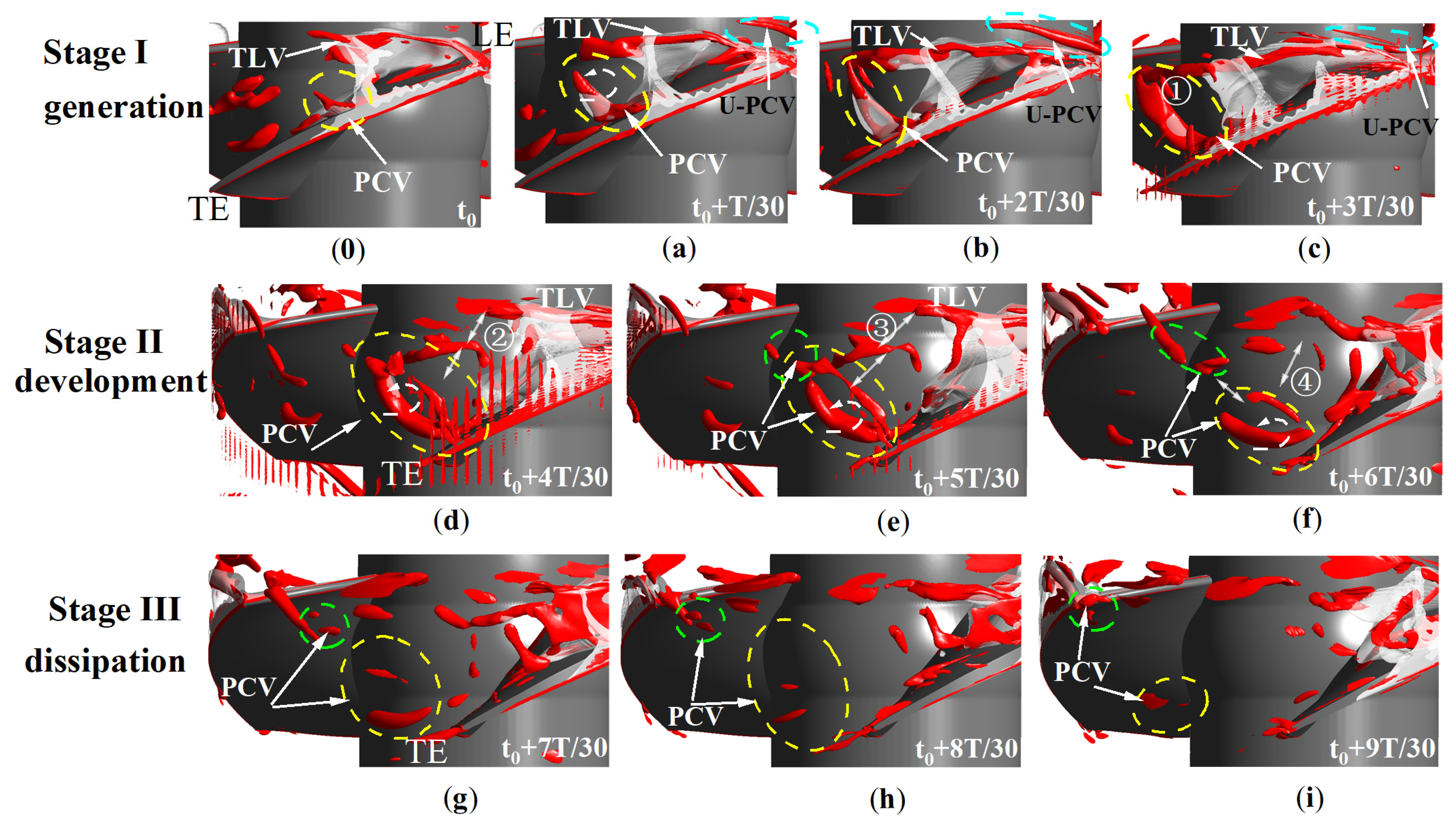
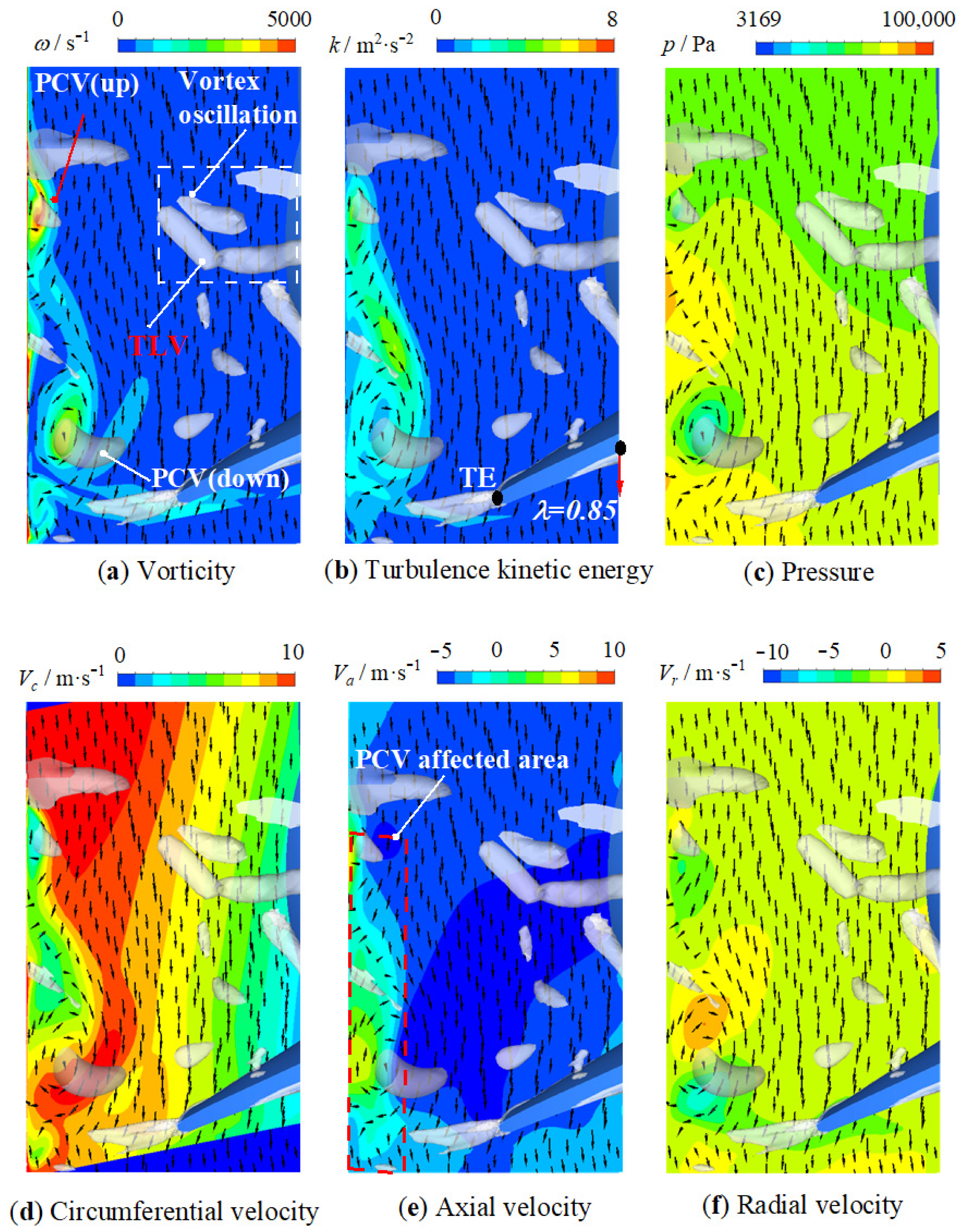
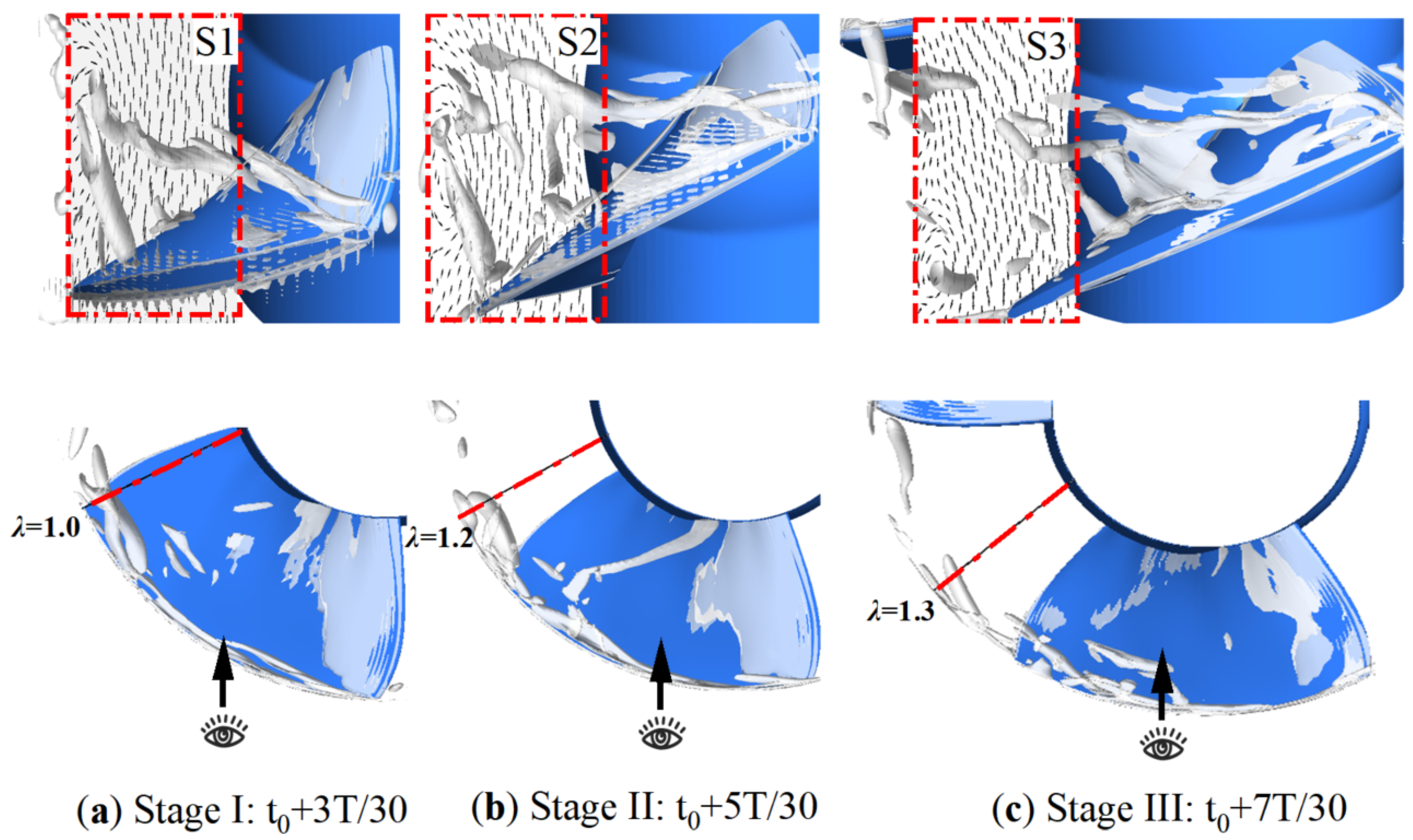
4.2. PCV’s Vortex Structure and Evolution Process

Through numerical simulation, the formation and evolution of the PCV can be further understood and analyzed. Figure 8 shows the vortex structure distribution in the clearance leakage flow field at different times, which was plotted using the isosurface with a swirling strength Sw equal to 1000 s⁻¹ and the isosurface with a cavitation volume fraction α_v equal to 0.1. Overall, the shape of the vortex structure was consistent with that in the experiment. The evolution of the PCV was further analyzed and explained.

Stage I: PCV generation.

At t₀, it was observed that there was an obvious PCV initiation phenomenon (surrounded by the yellow dotted line) in the middle of the blade. The vortex tended to rise upward, re-orient, and roll up the cavities on the blade surface, and it had the prototype of the PCV. At t₀ + 2T/30, the vortex grew further, almost perpendicular to the chord direction of the blade; the cavities carried by it were raised, and the cavitation was also significantly enhanced. At t₀ + 3T/30, the vortex and the cavities were stable and enhanced, and the morphology was close to that of the PCV observed in the experiment. The cyan dotted line in the figure shows the residual PCV of the upper blade, which was cut by the leading edge of the current blade and gradually integrated into the TLV; so, the TLV was temporarily enhanced. Interestingly, it can be clearly seen at position ① in Figure 8c that the PCV collided with the TLV, and they were mixed and entrained with each other.

Stage II: PCV development.

After the PCV separated from the main cavitation zone and developed, it collided and entrained with TLV, as shown in Figure 8c. The PCV for the current blade has the same scale as the TLV, but the vortex intensity was weak because the TLV was in the tail edge dissipation state. As can be seen in Figure 8d, the vortex structure at the tail of the TLV was stripped out of the main body and pulled to the PCV side by entrainment. This process is represented by ① → ② → ③ → ④ in the figure. The process lasted for a long time. Finally, Figure 8f shows that the vortex structure in the second half of the TLV was broken and mixed with the PCV part, while the PCV was gradually divided into two parts in this process. The upper part (green dotted line part) moved along the TLV direction by entrainment, combined with the residual part of the TLV, and was finally captured by the leading edge of the next blade. The lower part (yellow dotted line part) was far away from the TLV and was less affected by the TLV; so, the lower PCV continued to move and develop along the circumferential and axial direction, and finally left the impeller area.

Stage III: PCV dissipation.

Due to the weakening and dissipation of the TLV, the PCV was weakened by its upward entrainment, which changed the original state of the PCV perpendicular to the chord length and gradually developed and evolved along the circumferential horizontal direction. In the process of collision and mixing with the TLV, the PCV itself split into two parts. The upper part of the PCV collided with the leading edge of the next blade and then integrated with and participated in the evolution cycle of the next blade. After the lower part of the PCV left the trailing edge of the blade, the supplement of the leakage flow and its vortex was obviously weakened, and it was subjected to pressure oscillation at the trailing edge, resulting in its rapid dissipation.

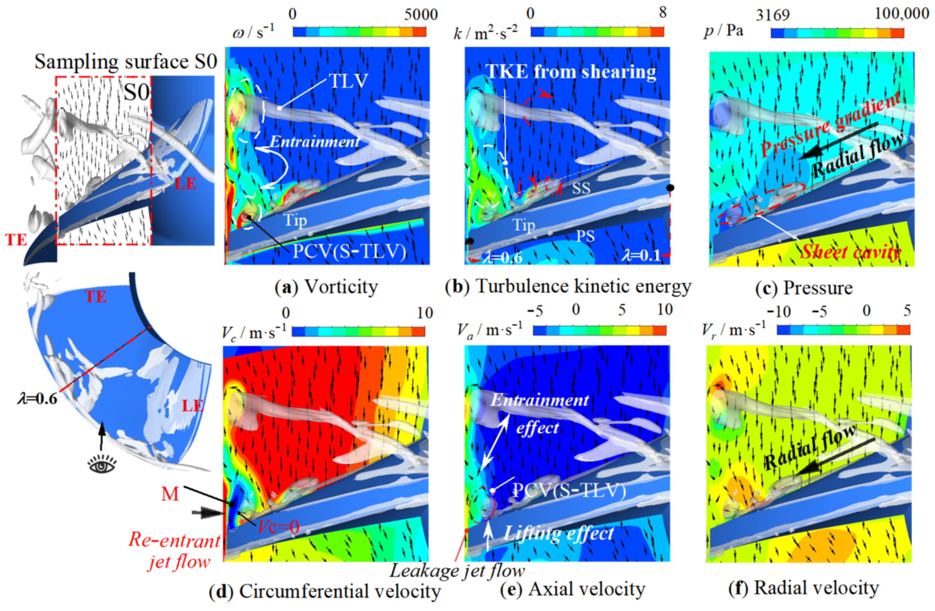
4.3. PCV Formation and Evolution Mechanism

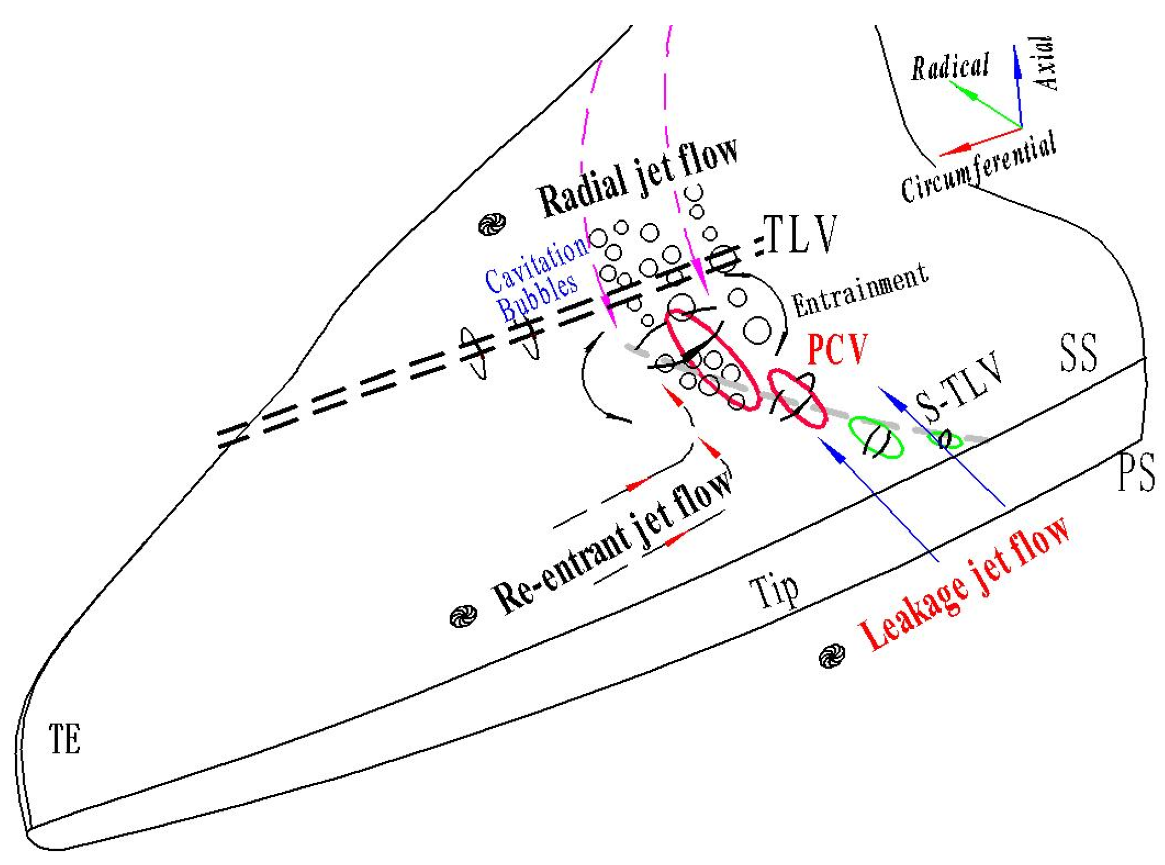
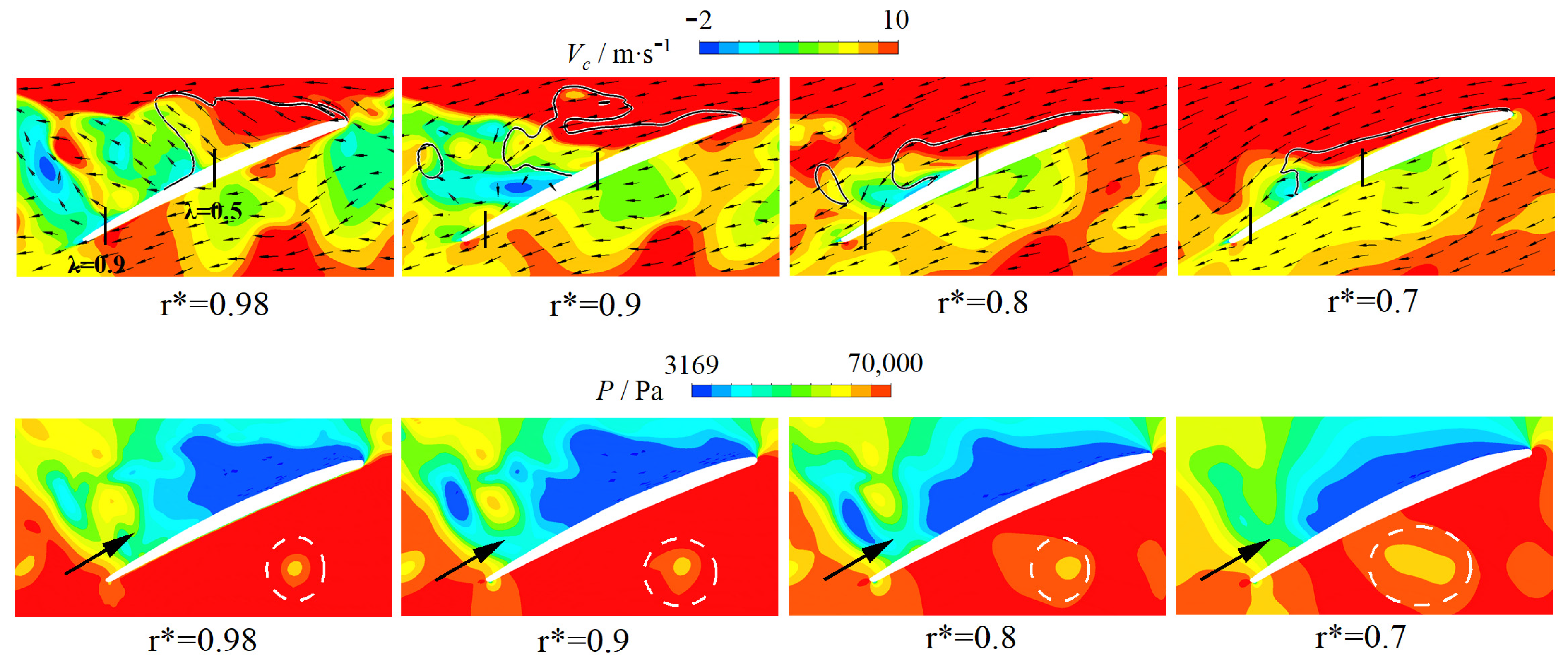
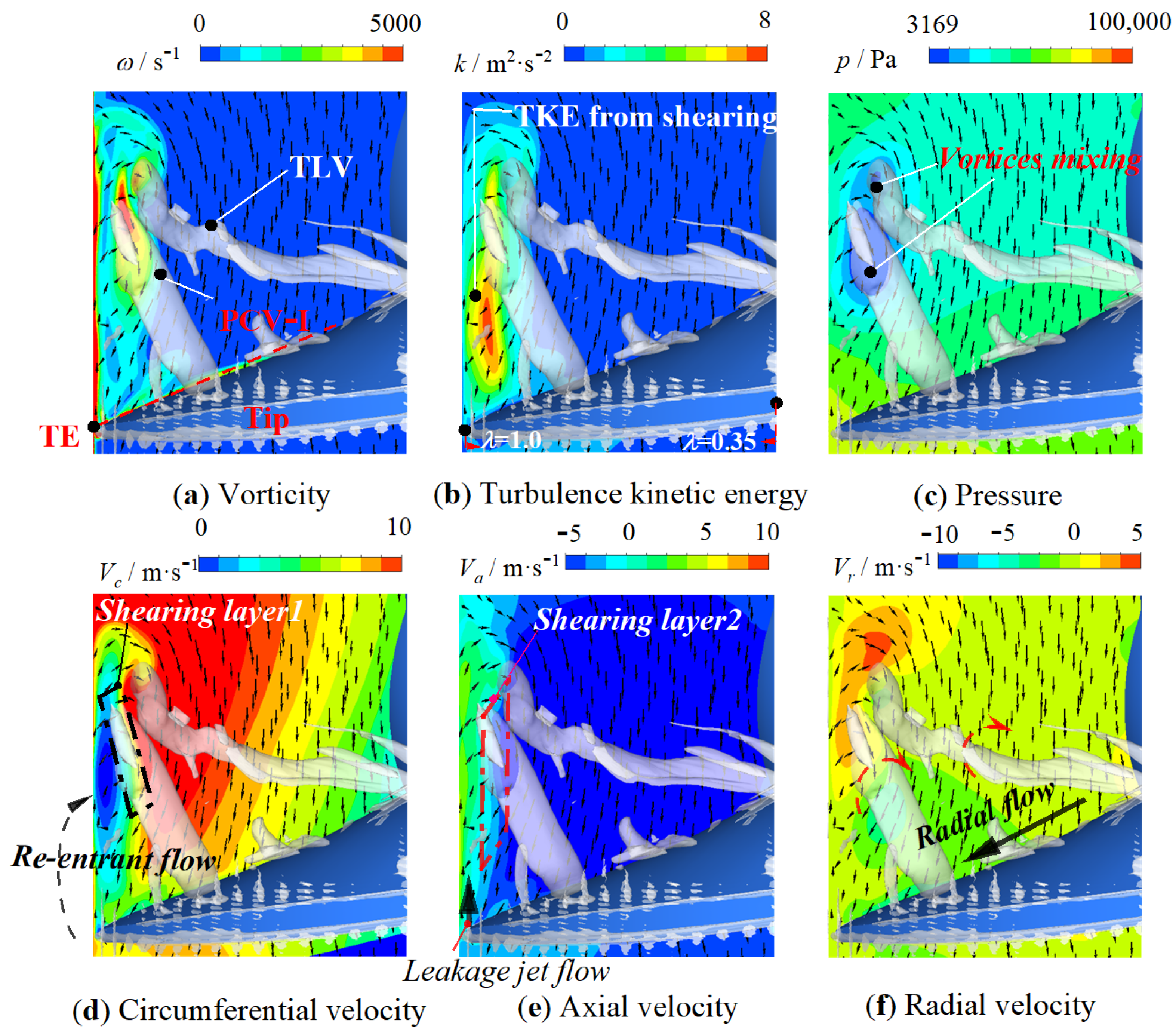
4.3.1. PCV Formation Mechanism

The PCV was composed of cavitation bubbles and vortices. Firstly, the respective sources of vortices and cavitation bubbles were analyzed, and then, the dynamic mechanism of the evolution of the cavitation vortices was analyzed. For the convenience of explanation, the moment t = t₀ + T/30 was taken as an example for explanation. The distribution of the physical quantities at that moment is shown in Figure 9, which mainly shows the distribution of the physical quantities such as the vorticity, turbulent kinetic energy, pressure, and circumferential, axial, and radial velocities on the sampling plane S0.

The source of the vortex: The PCV was generated near the tip of the blade in the middle of the chord, and the fluid on the suction side was sheared by the leaking jet to form a Secondary tip leakage vortex (S-TLV), as shown in Figure 9a,e. Its formation mechanism was consistent with the formation mechanism of the TLV. At the same time, due to the influence of the re-entrant jet, the circumferential velocity of the fluid near the tip clearance at M in Figure 9d was small, close to zero; so, the vortex formed by the leaking jet (S-TLV) could not follow in the circumferential direction with the rotation of the impeller, but rather gradually accumulated at M.

The source of cavitation bubbles: Driven by the radial pressure gradient, the radial jet pushed the sheet-like cavitation bubbles above the suction surface to the blade tip.

Mixing of cavitation and vortex: The cavitation bubbles pushed by the radial jet and the formed S-TLV were mixed with each other at M to form a cavitation vortex (CV), and the turbulent kinetic energy at this position was relatively large, as shown in Figure 8b.

PCV formation and movement mechanism: With the action of the leaking jet, the CV gradually rose, and with the combined action of the entrainment of the TLV, the CV moved upward in the axial direction and in the radial direction of the hub. The PCV vortex shape gradually became perpendicular to the chord length direction.

Figure 10 shows the schematic diagram of the initial stage of the PCV. As shown in the figure, the S-TLV was initially formed in the middle of the blade with the action of the leakage jet flow, and then, the S-TLV was squeezed by the re-entrant jet flow to stay at a certain position and combined with the cavitation bubbles pushed by the radial jet flow to form a CV. Then, the PCV vortex structure was formed under the effect of the uplift of the leakage flow and the entrainment of the TLV. Simply put, the formation of the PCV required the combination of the jet flow in three directions, the sheet cavitation conditions, and TLV vortex entrainment. The formation mechanism of the S-TLV, re-entrant jet flow, and radial jet flow was then further analyzed, as explained below.

4.3.2. Formation Mechanism of S-TLV

When the cavitation number was low, the cavitation degree at the leading edge of the blade was relatively strong. The mixing of the cavitation bubbles and vortices increased the height of the TLV vortex core, reducing the vortex intensity and the TLV entrainment capacity [42]. As a result, the vortex that formed at the rear of the blade could independently form the S-TLV, as shown in Figure 11. Under the standard flow conditions, the flow field was more stable, and it was easier to capture the S-TLV.

Figure 11 shows the schematic diagram of the S-TLV under standard flow conditions, shown by the numerical simulation and experimental results. In the subgraph of the numerical simulation, the vortex structure is identified by the swirling strength isosurface. It could be seen in the figure that the S-TLV formed with different cavitation numbers. When the cavitation number was lower, the leakage velocity was greater, and the height of the leakage vortex center was higher (H1 > H2 > H3). As the cavitation number decreased, the S-TLV scale gradually increased.

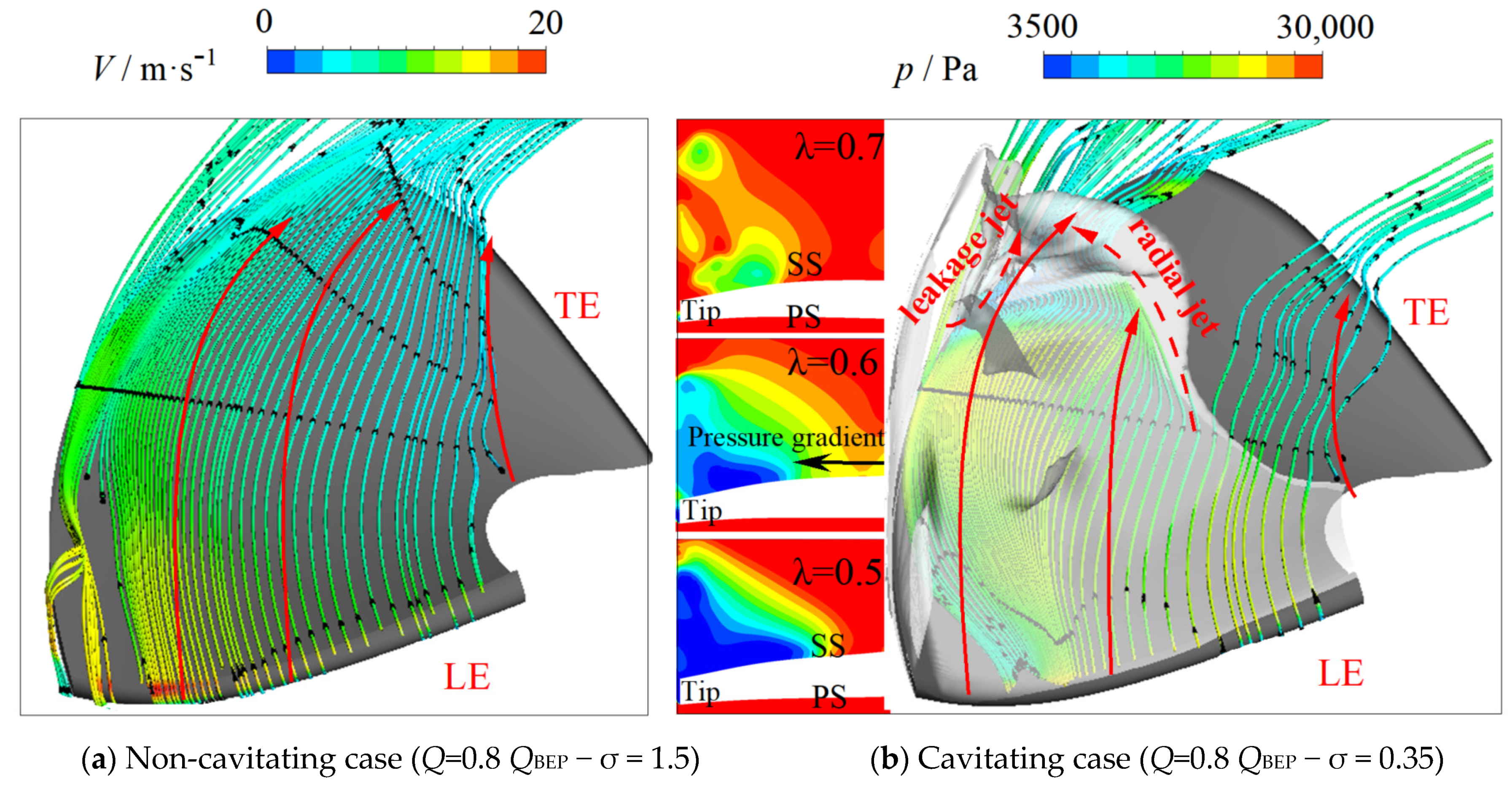
4.3.3. The Source of the Radial Jet Flow

Figure 12 shows the comparison diagram of the surface streamlines and the cavitation volume fraction isosurface (α_v = 0.1) on the blade suction surface of the non-cavitating case and the cavitating case. As shown in Figure 12b, the streamline direction at the cavitation boundary was deflected, producing a strong radial jet flow and pushing the sheet-like cavitation bubbles to S-TLV to form a PCV. This was because the cavities changed the original pressure distribution of the blade on the suction surface. The formation of the radial jet was caused by pressure gradients in the radial directions. When the fluid entered the high-pressure area at the trailing edge from the low-pressure area of the leading edge cavitation, the fluid was blocked, and it moved along the cavitation boundary line. This movement formed a radial jet flow.

4.3.4. The Source of the Re-entrant Jet Flow

Under the condition of a low cavitation number, sheet-like or even cloud-like cavities were formed above the suction surface of the leading edge of the blade, which caused the fluid in the middle and rear parts of the blade suction surface to flow slowly in the circumferential direction.

Figure 13 shows the distribution of the circumferential velocity and pressure in the radial sections. At the position of λ = 0.5–0.9, there was a significant decrease in circumferential direction velocity, even backflow, and the r* = 0.9 section was the most obvious. At the same time, cavitation occurred at the leading edge of the blade to form a low-pressure zone. Correspondingly, the trailing edge was a high-pressure zone; so, a pressure gradient was formed at the rear of the blade, driving the fluid at this position to form a re-entrant jet flow.

Due to the effect of the spin of the PCV, a recirculation zone appeared above the suction surface of the trailing edge of the r* = 0.98 section, confirming the influence zone of the PCV. There was a local low pressure area on the PS side of the blade (white dashed area), which might have been the residual part of the PCV formed by the last blade. This would have a certain impact on the stability of the blade, and it was difficult to capture this phenomenon in experiments.

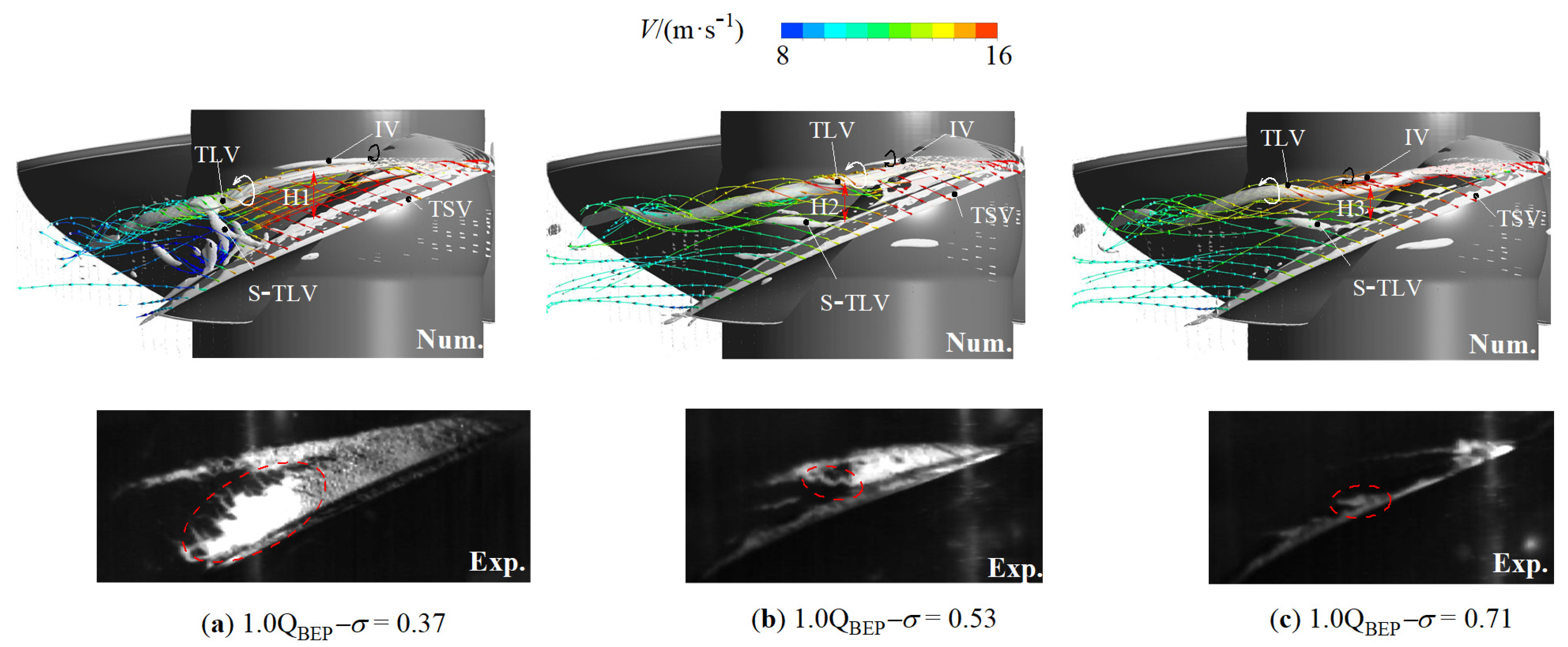
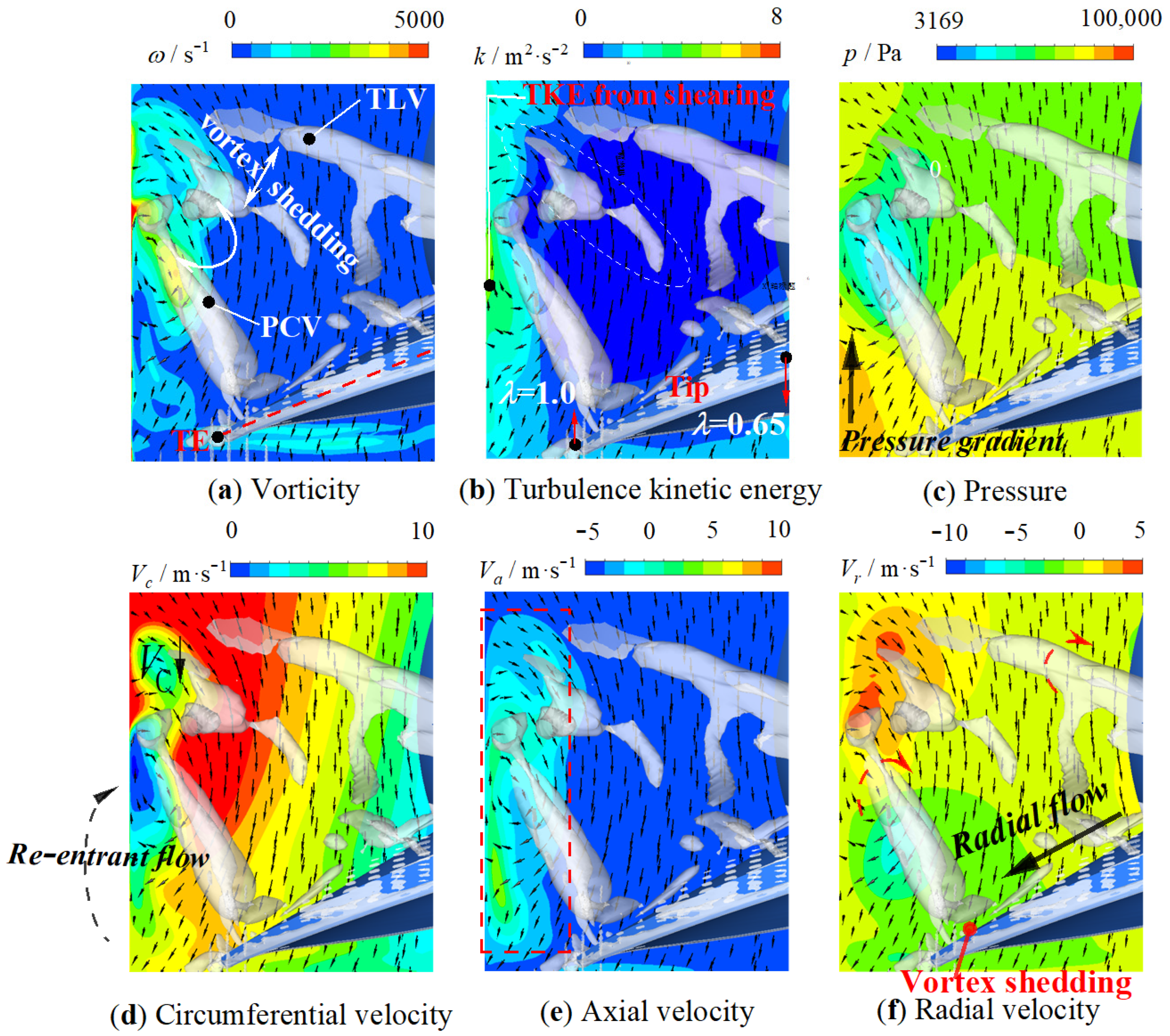
4.3.5. PCV’s Evolution Mechanism

Three moments of t₀ + 3T/30, t₀ + 5T/30 and t₀ + 7T/30, corresponding to three stages, were taken, and the evolution process of the PCV was analyzed. The physics of the three sections S1, S2, and S3 in the red dotted box in Figure 14 was analyzed. As shown in the figure, there were plane streamlines and swirling strength isosurfaces (Sw = 1000 s⁻¹) in the sections. In order to highlight the vortex structure, the swirling strength isosurface is colored white; at the same time, in order to obtain a 3D display and facilitate analysis, the observation angle is not perpendicular to the sampling surface.

Stage I: PCV generation

At t = t₀ + 3T/30, the physical quantity of the S1 plane shown in Figure 14a was taken for analysis, as shown in Figure 15. The PCV was developing downstream, and the vortex structure was becoming stronger, basically consistent with TLV on the vortex scale. At the same time, the PCV and TLV were mutually entrained, and the two vortices were mixed and fused at the position shown in the figure. Shear layer 1 was formed because of the convection between the re-entrant jet flow and the circumferential flow, which enhanced the vorticity of the PCV.

Furthermore, the axial convection between the leakage flow and the main flow formed shear layer 2, as shown in Figure 15e. The shear vorticity formed in this process gradually supplied the PCV and increased the axial vorticity of the PCV. Therefore, in this stage, the PCV developed gradually and vortex strength increased.

Stage II: PCV development and evolution

At t = t₀ + 5T/30, the physical quantity of the S2 plane shown in Figure 14b was taken for analysis, as shown in Figure 16. The PCV then broke away from the blade and further developed downstream. The vortices gradually dissipated and shrank in scale. At the same time, the PCV and TLV still entrained each other, and the PCV was slightly stronger than the TLV. The vortex structure of the TLV was obviously broken, and the PCV absorbed the vortex structure of the shedding part of the TLV. In addition, the radial flow impinged on the root of the PCV and made it shed from the suction surface of the blade, as shown in Figure 15f and Figure 16f.

Due to the effect of the wake vortex formed by the trailing edge of the blade, there was a certain re-entrant flow, as shown in Figure 16d. Because the leakage flow was at a certain angle with the chord length, the PCV in the wake of the blade was still affected by the leakage flow, where the TKE formed by the convective shear in the axial direction between the leakage flow and the main flow. Due to the low flow rate of the leakage flow at the tail, the vorticity transport formed by shear can only maintain the shape of PCV, as shown in Figure 16.

Stage III: PCV dissipative collapse

At t = t₀ + 7T/30, the physical quantity of the S3 plane shown in Figure 14c was taken for analysis, as shown in Figure 17. The PCV had separated from the blade and further developed downstream. The vorticity of the PCV was stronger than that of the TLV, and the vortex structure of the TLV had the form of vortex oscillation fragmentation and dissipation. The PCV absorbed the broken vortex structure of the TLV. The PCV was divided into two parts: the upper part and the lower part. Because the position of PCV was close to the trailing edge of the blade, as shown in Figure 17a, there was still some leakage jet flow, which caused the vorticity of the PCV to remain stable.

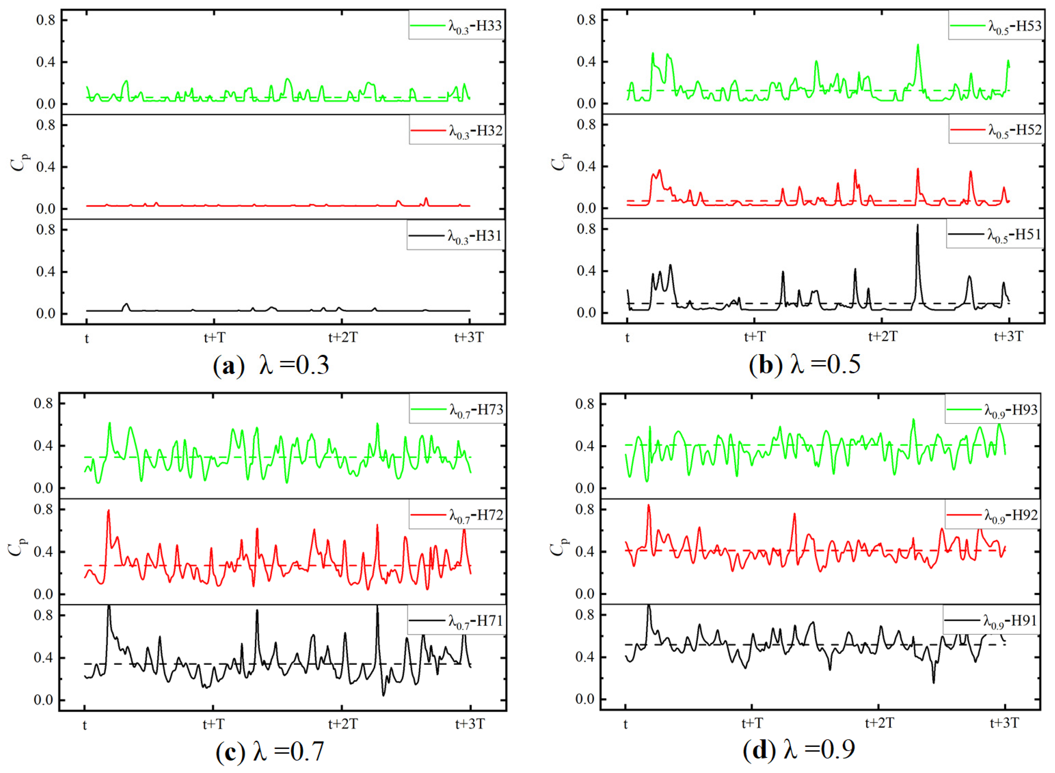
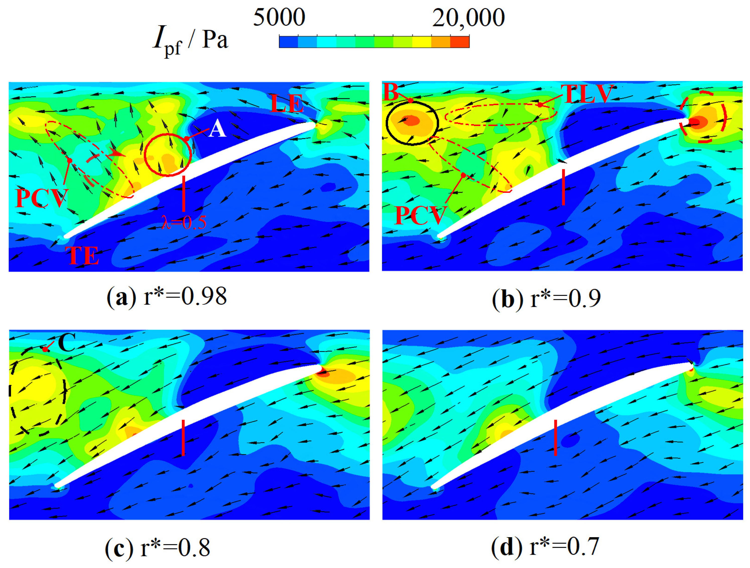
4.4. Pressure Fluctuation

The intensity of the pressure fluctuation $I_{\mathrm{p}}{}_{\mathrm{f}}$ was defined as follows [43]:

$$\overline{p}=\frac{1}{N}{\displaystyle \sum _{i=1}^N{p}_i}$$

(8)

$$I_{\mathrm{p}}{}_{\mathrm{f}}=\sqrt{\frac{1}{N}{\displaystyle \sum _{i=1}^N{}_i}{(p_i-\overline{p})}^2}$$

(9)

where $p_{\mathrm{i}}$ is the pressure at each time step, $\overline{p}$ is the arithmetic average of the pressure, and N is the sample number.

The calculation result of the last circle was taken as the sampling point for calculation, and the $I_{\mathrm{p}}{}_{\mathrm{f}}$ distribution was obtained as shown in Figure 18. For the section with r* = 0.98, it was observed that the pressure pulsation had a maximum value near λ = 0.5, which coincided with the place where the PCV was generated. It belonged to the area where the cavitation detachment and vortex generation were relatively strong. This showed that the PCV was generated near the tip of the blade, which further proved that the PCV originated from the S-TLV.

In the cross-section of r* = 0.9, the pressure pulsation at λ = 0.5 near the suction surface was still large. Strong pressure pulsation appeared at the LE, indicating that the U-PCV of the previous blade was captured and cut by the blade, which was consistent with the phenomenon observed in the experiment. In addition, the pulsation peak at the high place of area B in Figure 18b was caused by the mixing and entrainment interaction between the PCV and TLV, which caused the pressure pulsation at this position to be larger.

The pressure pulsation of the r* = 0.8 and 0.7 sections decreased, indicating that the influence of the PCV on these two sections was reduced, reflecting the fact that the main influence range of the PCV was near the tip region. In Figure 18c, there was a high pressure pulsation intensity in region C, indicating that this position was still affected by the mixing of the TLV and the PCV. As shown in Figure 18c,d, there was still a strong pressure pulsation between λ = 0.5 and λ = 0.7 near the suction surface, which was likely caused by the shedding of the sheet cavitation. The influence of the PCV was not visible, but the cavity at this position was pushed to the blade tip by the action of the radial flow.

In addition, for the r* = 0.98 section, Figure 19 shows the set pressure monitoring points. In the calculation setup, these points followed the rotation of the impeller and their positions remained unchanged relative to the blade.

The obtained pressure coefficient curves are shown in Figure 20, and the dotted line in the figure is the average value of the pressure coefficient.

As shown in Figure 20a, the pressure coefficient of H31/H32 remained the lowest value, indicating that a large amount of cavitation was generated and grew steadily, and the pressure began to pulsate at H33, indicating that the height was the cavitation boundary area, where the cavitation bubble seemed to experience a small rupture.

As shown in Figure 20b, the periodicity of the pressure pulsation at each monitoring point was essentially the same. Because there was still a large amount of cavitation above the suction surface at this location, the valley value could reach the saturated vapor pressure of cavitation.

The monitoring points H51 and H52 had low vibration frequency, which was due to the periodic shedding at the circumferential boundary of the sheet cavity above the suction surface. This chord position was also the initial stage of PCV formation, and the radial jet pushed the cavity to the tip of the blade. The interaction between the vortex and the cavitation caused the large amplitude pressure pulsation phenomenon at the monitoring point H51. The monitoring point H53 was located at the axial boundary of the cavity. The frequency of the pressure pulsation caused by cavitation rupture was high, but the pulsation amplitude was small.

As shown in Figure 20c,d, these positions had basically been separated from the main cavitation zone, and the average pressure had risen. However, due to its location at the trailing edge, the pressure pulsation vibration frequency was aggravated due to the impact of the re-entrant jet flow, the upstream cavitation shedding, and the rupture. At the same time, due to the effect of the mutual entrainment, mixing, evolution, and dissipation of the PCV and TLV, the pressure pulsation presented a certain periodicity. The frequency of the pressure pulsation at the trailing edge was higher than that at the leading edge of the blade. The pressure pulsation amplitude of the monitoring point at λ = 0.7 was the largest. The average value of the pressure coefficient gradually increased along the chord length; so, the collapse of the cavitation bubbles was accelerated.

5. Conclusions

In this work, the PCV was found to originate from S-TLV. With the blocking effect of the re-entrant jet, the PCV gathered in the middle of the blade and combined with the cavitation bubbles driven by the radial flow to form a CV. With the combined action of the tip leakage jet lifting and TLV entrainment, the CV was re-oriented and gradually became perpendicular to the chord length, forming the PCV.

The evolution of the PCV was divided into three stages: generation, development, and dissipation. In this process, the PCV and TLV collided, mixed, and entrained each other. Finally, the PCV was divided into the upper and lower parts. The upper part was combined with the residual part of the TLV and then flowed to the next blade, and the lower part flowed out of the impeller area along the axial direction.

The numerical simulation captured the interesting flow details of collision, entrainment, and fragmentation between the PCV and TLV, and vividly illustrated the process of mutual entrainment and the tearing of the vortices.

The influence area of the PCV was mainly near the blade tip (r* = 0.7–1) in the middle and rear above the blade, where the intensity and the frequency of the pressure fluctuation were high.

References

1. Guan, X. Axial Flow Pump and Mixed Flow Pump; Aerospace Press: Beijing, China, 2009. [Google Scholar]
2. Rains, D.A. Tip Clearance Flows in Axial Compressors and Pumps. Ph.D. Thesis, California Institute of Technology, Pasadena, CA, USA, 1954. [Google Scholar]
3. Miorini, R.L.; Wu, H.; Katz, J. The internal structure of the tip leakage vortex within the rotor of an axial Water jet pump. J. Turbomach. 2012, 134, 031018. [Google Scholar] [CrossRef]
4. Zhang, H.; Zuo, F.; Zhang, D.; Shi, W. Formation and Evolution Mechanism of Tip Leakage Vortex in Axial Flow Pump and Vortex Cavitation Analysis. Trans. Chin. Soc. Agr. Mach. 2020, 52, 157–167. [Google Scholar]
5. Wu, H.; Miorini, R.L.; Tan, D.; Katz, J. Turbulence within the tip-leakage vortex of an axial waterjet pump. AIAA J. 2012, 50, 2574–2587. [Google Scholar] [CrossRef]
6. You, D.; Wang, M.; Moin, P.; Mittal, R. Large-eddy simulation analysis of mechanisms for viscous losses in a turbomachinery tip-clearance flow. J. Fluid Mech. 2007, 586, 177–204. [Google Scholar] [CrossRef] [Green Version]
7. Doligalski, T.L.; Smith, C.R.; Walker, J.D.A. Vortex Interactions with Walls. Annu. Rev. Fluid Mech. 1994, 26, 573–616. [Google Scholar] [CrossRef]
8. Guo, Q.; Zhou, L.; Wang, Z. Numerical evaluation of the clearance geometries effect on the flow field and performance of a hydrofoil. Renew. Energy 2016, 99, 390–397. [Google Scholar] [CrossRef]
9. Shi, L.; Zhang, D.; Jin, Y.; Shi, W.; van Esch, B.P.M. A study on tip leakage vortex dynamics and cavitation in axial-flow pump. Fluid Dyn. Res. 2017, 49, 035504. [Google Scholar] [CrossRef]
10. Liu, Y.; Tan, L. Method of C groove on vortex suppression and energy performance improvement for a NACA0009 hydrofoil with tip clearance in tidal energy. Energy 2018, 155, 448–461. [Google Scholar] [CrossRef]
11. Tran, B.N.; Jeong, H.; Kim, J.H.; Park, J.-S.; Yang, C. Effects of Tip Clearance Size on Energy Performance and Pressure Fluctuation of a Tidal Propeller Turbine. Energies 2020, 13, 4055. [Google Scholar] [CrossRef]
12. You, D.; Wang, M.; Moin, P.; Mittal, R. Vortex Dynamics and Low-Pressure Fluctuations in the Tip-Clearance Flow. J. Fluids Eng. 2007, 129, 1002–1014. [Google Scholar] [CrossRef]
13. You, D.; Wang, M.; Moin, P.; Mittal, R. Effects of tip-gap size on the tip-leakage flow in a turbo machinery cascade. J. Phys. Fluids 2006, 18, 105102. [Google Scholar] [CrossRef] [Green Version]
14. Zhang, H.; Zuo, F.; Zhang, D.; Shi, W. Formation mechanism and geometric influence of tip clearance vortex structure around hydrofoil. J. Zhejiang Uni. (Eng. Sci.) 2020, 54, 2344–2355. [Google Scholar]
15. Giuni, M.; Green, R.B. Vortex formation on squared and rounded tip. Aerosp. Sci. technol. 2013, 29, 191–199. [Google Scholar] [CrossRef] [Green Version]
16. Moghadam, S.; Meinke, M.; Schröder, W. Analysis of tip-leakage flow in an axial fan at varying tip-gap sizes and operating conditions. Comput. Fluids 2019, 183, 107–129. [Google Scholar] [CrossRef]
17. Hsiao, C.T.; Chahine, G.L. Scaling of tip vortex cavitation inception noise with a bubble dynamics model accounting for nuclei size distribution. J. Fluids Eng. 2005, 127, 55–65. [Google Scholar] [CrossRef]
18. Chen, H.; Doeller, N.; Li, Y.; Katz, J. Experimental Investigations of Cavitation Performance Breakdown in an Axial Waterjet Pump. J. Fluids Eng. 2020, 142, 091204. [Google Scholar] [CrossRef]
19. Qiu, C.; Huang, Q.; Pan, G.; Shi, Y.; Dong, X. Numerical simulation of hydrodynamic and cavitation Performance of pump jet propulsor with different tip clearances in oblique flow. Ocean Eng. 2020, 209, 107285. [Google Scholar] [CrossRef]
20. Geng, L.; Escaler, X. Assessment of RANS turbulence models and Zwart cavitation model empirical coefficients for the simulation of unsteady cloud cavitation. Eng. Appl. Comp. Fluid Mech. 2020, 14, 151–167. [Google Scholar] [CrossRef]
21. Dreyer, M. Mind the Gap: Tip Leakage Vortex Dynamics and Cavitation in the Axial Turbines. Ph.D. Thesis, Swiss Federal Institute of Technology in Lausanne (EPFL), Lausanne, Swiss, 2015. [Google Scholar]
22. Decaix, J.; Dreyer, M.; Balarac, G.; Farhat, M.; Münch, C. RANS computations of a confined cavitating tip-leakage vortex. Eur. J. Mech. B-Fluid. 2018, 67, 198–210. [Google Scholar] [CrossRef] [Green Version]
23. Chen, H.Y.; Bai, X.R.; Long, X.P.; Ji, B.; Farhat, M. Large eddy simulation of the tip-leakage cavitating flow with an insight on how cavitation influences vorticity and turbulence. Appl. Math. Model. 2019, 77, 788–809. [Google Scholar] [CrossRef]
24. Guo, Q.; Huang, X.; Qiu, B. Numerical investigation of the blade tip leakage vortex cavitation in a waterjet pump. Ocean Eng. 2019, 187, 106170. [Google Scholar] [CrossRef]
25. Tan, D.; Li, Y.; Wilkes, I.; Vagnoni, E.; Miorini, R.L.; Katz, J. Experimental Investigation of the Role of Large Scale Cavitating Vortical Structures in Performance Breakdown of an Axial Waterjet Pump. J. Fluids Eng. 2015, 137, 111301. [Google Scholar] [CrossRef]
26. Zhang, D.; Shi, L.; Shi, W.; Zhao, R.; Wang, H.; Van Esch, B. Numerical analysis of unsteady tip leakage vortex cavitation cloud and unstable suction-side-perpendicular cavitating vortices in an axial flow pump. Int. J. Multiph. Flow 2015, 77, 244–259. [Google Scholar] [CrossRef]
27. Shi, L.; Zhang, D.; Zhao, R.; Shi, W.; Van Esch, B. Visualized observations of trajectory and dynamics of unsteady tip cloud cavitating vortices in axial flow pump. J. Fluid Sci. Technol. 2017, 12, JFST0007. [Google Scholar] [CrossRef] [Green Version]
28. Shen, X.; Zhang, D.; Xu, B.; Shi, W.; van Esch, B. Experimental and numerical investigation on the effect of tip leakage vortex induced cavitating flflow on pressure flfluctuation in an axial flflow pump. Renew. Energy 2021, 163, 1195–1209. [Google Scholar]
29. Shen, X.; Zhang, D.; Xu, B.; Jin, Y.; Shi, W.; Esch, B. Experimental investigation of the transient patterns and pressure evolution of tip leakage vortex and induced-vortices cavitation in an axial flflow pump. J. Fluid Eng. 2020, 142, 101206. [Google Scholar]
30. Zhang, D.; Shi, W.; Pan, D.; Dubuisson, M. Numerical and Experimental Investigation of Tip Leakage Vortex Cavitation Patterns and Mechanisms in an Axial Flow Pump. J. Fluids Eng. Trans. ASME 2015, 137, 121103. [Google Scholar] [CrossRef]
31. Dreyer, M.; Decaix, J.; Münch-Alligné, C.; Farhat, M. Mind the gap: A new insight into the tip leakage vortex using stereo-PIV. Exp. Fluids 2014, 55, 1849. [Google Scholar] [CrossRef]
32. Tan, D.Y.; Miorini, R.L.; Keller, J.; Katz, J. Flow Visualization Using Cavitation Within Blade Passage of an Axial Waterjet Pump Rotor. In Proceedings of the ASME 2012 Fluids Engineering Summer Meeting, Rio Grande, PR, USA, 8–12 July 2012. [Google Scholar]
33. Wu, H.; Miorini, R.L.; Katz, J. Measurements of the tip leakage vortex structures and turbulence in the meridional plane of an axial water-jet pump. Exp. Fluids 2011, 50, 989–1003. [Google Scholar]
34. ANSYS, Inc. ANSYS CFX-Solver Theory Guide, Release 17.1; SAS IP, Inc.: Canonsburg, PA, USA, 2016. [Google Scholar]
35. Menter, F.R. Review of the shear-stress transport turbulence model experience from an industrial perspective. Int. J comput. Fluid. D. 2009, 23, 305–316. [Google Scholar] [CrossRef]
36. Heydari, M.; Sadat-Hosseini, H. Analysis of propeller wake field and vortical structures using k-Omega SST Method. Ocean Eng. 2020, 204, 107247. [Google Scholar] [CrossRef]
37. Zhao, Y.; Wang, G.; Jiang, Y.; Huang, B. Numerical analysis of developed tip leakage cavitating flows using a new transport-based model. Int. Commun. Heat Mass Transf. 2016, 78, 39–47. [Google Scholar] [CrossRef]
38. Zhang, D.; Shi, W.; van Esch, B.; Shi, L.; Dubuisson, M. Numerical and experimental investigation of tip leakage vortex trajectory and dynamics in an axial flow pump. Comput. Fluids 2015, 112, 61–71. [Google Scholar] [CrossRef]
39. Smirnov, P.E.; Menter, F.R. Sensitization of the SST turbulence model to rotation and curvature by applying the Spalart-Shur correction term. J. Turbomach. 2009, 131, 041010. [Google Scholar] [CrossRef]
40. Spalart, P.R.; Shur, M. On the sensitization of turbulence models to rotation and curvature. Aerosp. Sci. Technol. 1997, 1, 297–302. [Google Scholar] [CrossRef]
41. Zwart, P.; Gerber, A.G.; Belamri, T. A two-phase model for predicting cavitation dynamics. In Proceedings of the ICMF 2014 International Conference on Multiphase Flow, Yokohama, Japan, 30 May–3 June 2004; p. 152. [Google Scholar]
42. Zhang, H.; Wang, J.; Zhang, D.; Shi, W.; Zang, J. Numerical Analysis of the Effect of Cavitation on the Tip Leakage Vortex in an Axial-Flow Pump. J. Mar. Sci. Eng. 2021, 9, 775. [Google Scholar] [CrossRef]
43. Liu, Y.; Tan, L. Tip clearance on pressure fluctuation intensity and vortex characteristic of a mixed flow pump as turbine at pump mode. Renew. Energy 2018, 129, 606–615. [Google Scholar] [CrossRef]
Figure 1. Axial flow pump structure composition and geometric parameters.
Jmse 09 01045 g001
Figure 2. Geometric definition of the impeller.
Jmse 09 01045 g002
Figure 3. Experimental equipment used the axial flow pump to examine the external characteristics and cavitation.
Jmse 09 01045 g003
Figure 4. Computational domain, mesh of the axial flow pump, and the y+ distribution on the blade surfaces.
Jmse 09 01045 g004
Figure 5. Time history curves of Cp with three different time steps (Q = 0.8 QBEP, σ = 0.35).
Jmse 09 01045 g005
Figure 6. Comparison of the axial flow pump’s σ–H curves from the numerical simulation and experiments (Q =0.8 QBEP).
Jmse 09 01045 g006
Figure 7. High-speed photography experimental diagram of axial flow pump impeller at different times (Q = 0.8 QBEP, σ = 0.35).
Jmse 09 01045 g007
Figure 8. Transient evolution of PCV and cavitation obtained via simulation (swirling strength isosurface Sw = 1000 s−1 (red), and the cavitation volume fraction isosurface αv = 0.1 (white), Q = 0.8 QBEP, σ = 0.35).
Jmse 09 01045 g008
Figure 9. Distribution of plane physical quantities in the initial stage of the PCV at t = t0 + T/30 (swirling strength isosurface Sw = 1000 s−1 (white), Q = 0.8 QBEP, σ = 0.35).
Jmse 09 01045 g009
Figure 10. Schematic diagram of the initial stage of the PCV.
Jmse 09 01045 g010
Figure 11. Schematic diagram of S-TLV under standard flow conditions, as shown by numerical simulation and experimental results.
Jmse 09 01045 g011
Figure 12. Comparison of blade surface streamlines and cavitation distribution on the suction surfaces of the non-cavitating and cavitating cases.
Jmse 09 01045 g012
Figure 13. Distribution of circumferential velocity Vc and pressure on radial sections (the solid line is the contour of the cavitation volume fraction αv = 0.1, Q = 0.8 QBEP, σ = 0.35).
Jmse 09 01045 g013
Figure 14. Schematic diagram of the physical quantity of the sampling surface at different moments (swirling strength isosurface Sw = 1000 s−1 (white), Q = 0.8 QBEP, σ = 0.35).
Jmse 09 01045 g014
Figure 15. Distribution of plane physical quantities in the stage of vortex generation at t = t0 + 3T/30 (swirling strength isosurface Sw = 1000 s−1 (white), Q = 0.8 QBEP, σ = 0.35).
Jmse 09 01045 g015
Figure 16. Distribution of plane physical quantities in the stage of vortex development and evolution at t = t0 + 5T/30 (swirling strength isosurface Sw = 1000 s−1 (white), Q = 0.8 QBEP, σ = 0.35).
Jmse 09 01045 g016
Figure 17. Distribution of plane physical quantities in the stage of vortex dissipative collapse at t = t0 + 7T/30 (swirling strength isosurface Sw = 1000 s−1 (white), Q = 0.8 QBEP, σ = 0.35).
Jmse 09 01045 g017
Figure 18. Distribution of the intensity of pressure fluctuation on radial sections (Q = 0.8 QBEP, σ = 0.35).
Jmse 09 01045 g018
Figure 19. Schematic diagram of pressure pulsation monitoring points’ setting positions (r* = 0.98).
Jmse 09 01045 g019
Figure 20. The pressure coefficient curves at different monitoring points (Q = 0.8 QBEP, σ = 0.35).
Jmse 09 01045 g020