Article

Comparative Analysis of Environmental Contour Approaches to Estimating Extreme Waves for Offshore Installations for the Baltic Sea and the North Sea

1
Department of Earth Sciences, Uppsala University, Villavägen 16, SE-752 36 Uppsala, Sweden
2
Centre of Natural Hazards and Disaster Science, Department of Earth Sciences, Uppsala University, Villavägen 16, SE-752 36 Uppsala, Sweden
3
Department of Electrical Engineering, Uppsala University, Lägerhyddsvägen 1, SE-751 21 Uppsala, Sweden
4
Department of Energy and Technology, Swedish University of Agricultural Sciences, Lennart Hjelms väg 9, SE-756 51 Uppsala, Sweden
*
Author to whom correspondence should be addressed.
J. Mar. Sci. Eng. 2021, 9(1), 96; https://doi.org/10.3390/jmse9010096
Submission received: 18 December 2020 / Revised: 11 January 2021 / Accepted: 13 January 2021 / Published: 18 January 2021
(This article belongs to the Section Ocean Engineering)

Abstract

:
At the stage of design load analysis for offshore installations such as wave energy systems, a critical step is the determination of environmental cases to be evaluated for the definition of the characteristic design load. A commonly used methodology for load case selection, applied in multiple studies and recommended by technical specifications and guidelines, is the environmental contour approach. Here, 50-year environmental contours were generated for four study sites located in the North Sea, Skagerrak and the Baltic Sea by considering both observations and hindcast (model) data. For the construction of the contours, the well-established inverse first-order method (I-FORM) and a modified version using principal component analysis (PCA) were both examined. Furthermore, a 2-dimensional peaks-over-threshold (2D POT) method was evaluated. It was found that a version of the regular I-FORM was able to produce satisfactory contours which properly accounted for the highest waves. When using PCA, the dependency in the data was not properly captured by the probability functions under consideration. The 2D POT method, where applicable, was found to underestimate the extreme sea states. Comparisons between contours obtained from observations and hindcast data showed that the contours may differ substantially depending on the site and method, and thus care must be exercised when using hindcast data for such purposes.

1. Introduction

The advancement of offshore renewable energy technologies, such as offshore wind or wave energy technologies, towards commercial viability demands that methods for determining extreme environmental loads are further developed. In this paper, the focus is on determining environmental conditions to evaluate extreme loads for wave energy converters (WECs). The authors of Coe et al. [1] define extreme conditions as met-ocean conditions causing unusually large stress on the WEC system. The loading on a device can be 100 times higher than the average loading in extreme weather conditions [2], which provides a significant challenge to the structural design and consequent capital costs. Simultaneously, cost-effective design demands that the considered loads are without overestimation; therefore, accurate prediction of the characteristic design load is of high importance.
The methodology of WEC design includes many techniques adopted from oil and gas offshore technology as well as shipping; however, due to the dynamics and small scale of offshore renewable systems, the physical functioning of most of the WEC systems is different from such traditional offshore structures, and established results from the oil and shipping industry cannot be readily translated [1,3]. The WECs are designed to maximize the energy production, implying that WECs are often highly dynamical and operate close to resonance with the waves. A small number of standards and technical specifications are available for WEC design, useful guidelines are provided in IEC TS 62600-2 [4], N-003 [5], and DNV-RP-C205 [6].
However, identifying extreme conditions is a nontrivial task. In both numerical [7,8] and experimental [9,10] studies, it has been confirmed that the largest load on the devices may not be caused by the highest waves, and there may be load extremes related to a combination of the motion history and certain wave period and height combinations [7,11,12].
There are several methods for the evaluation of extreme ocean waves and several studies are focused on their comparison [13,14]. In particular, the univariate extreme value analysis considers the maximum significant wave height for a specified return period applying the peak-over-threshold (POT) approach or annual maxima method. However, it is important to consider the wave loading as the combination of several parameters, making the bivariate analysis to be a widely applied method in the design stage. The wave period cannot be neglected during the design of wave energy conversion systems, justifying the fact that the environmental contour is a widely applied approach for the design sea state selection as it is numerically less expensive and provides reliable estimations [15,16,17]. The authors of Coe et al. [18] summarized the standard methodologies for the selection of the design environmental conditions: (1) all sea states approach, (2) environmental contour approach, and (3) 1D design load selection. Figure 1 displays different steps involved in determining the characteristic load, starting from the environmental data. For a more exhaustive workflow which includes additional steps in the WEC design process, see Figure 1 in Coe et al. [18]. For WEC applications, a 50-year environmental contour is commonly used [18]. Following the methodology described in Coe et al. [18] regarding the evaluation of the design loads, several sea states along the contour are selected for further analysis. Each sea state is characterized by the significant wave height, wave period, and wave spectrum. Numerical modeling and/or experimental testing is conducted (see Figure 1), reproducing the selected sea states in order to investigate the wave–structure interaction under extreme wave conditions. The sea state for which the WEC has the largest response can be considered as the extreme design load, which can be evaluated against the structural capacity. The goal is to ensure that the WEC design being considered can withstand the environmental conditions of a specific site, while minimizing the structural cost [18]. For the industrial success of WEC technologies, survivability under extreme wave conditions is important as it is the key cost driver during the construction process. The present study focuses on the environmental contour approach and evaluates environmental data from both observations and hindcast models.
The traditional approach for creating environmental contours uses the Inverse-First Order Reliability Method (I-FORM) [19] and is recommended in the DNV standards [6]. This approach requires the development of a joint probability distribution model of the ocean parameters and then the I-FORM is applied for the definition of the environmental contour for a target exceedance probability. The correlation between the inputs is captured though a Rosenblatt [20] or Nataf [21] transformation. A Monte Carlo approach of a joint probability model to develop environmental contours has recently been published [22,23]. However, the Monte Carlo method has been found to yield unreasonable results for mixed sea systems, i.e., a combination of wind sea and swell, so the continued use of traditional Rosenblatt approach based on I-FORM is still warranted [14]. The I-FORM for the environmental contours definitions includes fitting distributions and models for the significant wave height and period. In many applications, the marginal distribution of significant wave height is modeled through a 3-parameters Weibull distribution [22,23,24,25] but it seems to misrepresent the upper tail of the distribution [13]. The interdependency of the significant wave height and wave period is captured through a joint log-normal distribution as suggested by Haver and Winterstein [26] and is also applied in [22,23,24,25].
Eckert-Gallup et al. [27] proposed techniques for improving the traditional I-FORM using principal component analysis (PCA) and enhanced extreme value models. The PCA generates variables which are uncorrelated and sorted such that the first variable represents the direction with largest variance data and each subsequent variable leads to the next largest variance. The new variables are called principal components. In particular for the creation of the environmental contour, PCA was applied to remove the correlation between the energy or peak period and significant wave height, resulting in two new variables named component one and component two, where component one has the largest variance. Applying PCA, more realistic representations of environmental contours of extreme sea states are expected, but at the same time the method is sensitive to the distribution fitting of the components.
Extreme sea states are not only important in the design of offshore renewable energy structures, but also in the operation and maintenance and site selection process [28,29]. Such considerations further highlight the importance of understanding and characterizing extreme sea states. A recent publication by Neary et al. [30] compared environmental contours for buoy observations and different hindcast data sets for several locations on the West Coast and East Coast of USA with a focus on extreme sea states for WEC applications. They employed the I-FORM with PCA to estimate environmental contours, and found that the model data generally lead to smaller contours compared with those from observations and that estimates of extreme sea states with high H s were underestimated by the models. This highlights the fact that care must be taken when results from model data are interpreted.
As stated in Eckert et al. [31], there is a need to compare environmental contour methods both at a single site and also across several different sites in order to make environmental contours useful in practice. They make a comparison of several sites along the US coasts, while also highlighting the need to investigate other geographic regions. The Northern European basins are of interest for the installation of offshore renewable energy structures (RES), and thus environmental contour methods should be investigated in the Baltic Sea and North Sea. In the present work, several environmental contour methods are evaluated and compared for four sites located in Baltic Sea and North Sea.
To our knowledge there are no previous studies which evaluate environmental contour methods in the Baltic Sea region. In this region, extreme wave heights have been investigated (see, e.g., Björkqvist et al. [32]); however, for the design of offshore RES, additional wave parameters are of interest, such as the wave steepness (which depends on both wave height and period). For identification of extreme waves in North Sea, the environmental contour method has been applied based mainly using I-FORM [26,33,34]. However, the PCA method of Eckert-Gallup et al. [27] has not been investigated for the North Sea wave climate, which will be done in this study.
The present paper focuses on the prediction of extreme sea states—using a 50-year return period—for four study sites: Ölands Södra Grund in the Baltic Sea, Väderöarna in Skagerrak, and Tyne Tees, and Dowsing in the North Sea. For all the sites, both hindcast data and observations were considered.
The purpose of this study is twofold: one objective is, for a specific set of data, to evaluate different methods for constructing 50-year environmental contours. The second objective is to compare the contours obtained from observational and hindcast data. Such contour comparisons include numerical properties, such as the maximum significant wave height along the contour. However, there are several other important aspects to comparing different environmental contours for a specific site. First of all, it is sensible that the contour encloses the data in a reasonable way, e.g., if 10 years of data are used to construct a contour, it is unlikely that a sea state would exceed the 50-year environmental contour. However, if 50 years of data are used, it is reasonable that the environmental contour is not too far away from the outermost data points. As a second point, the environmental contour should capture the dependence between the two variables. Another aspect to keep in mind is that the sea states with high wave height is of special interest from a practical (design) viewpoint, and it is important that the environmental contour properly reflect these sea states.
For the environmental contours in this study, the classical I-FORM method was applied, as was the recent I-FORM modification developed by Eckert-Gallup et al. [27] where a coordinate transformation is used. Furthermore, a 2-dimensional peak-over-threshold (2D POT) method, commonly used in the study of compound extremes in, e.g., hydrology, was applied by considering high thresholds of wave height and wave steepness. A novel statistical approach to compare performance of methods for a range of return periods was also used.
This paper is organized as follows. Section 2 discusses the study sites and the different data sets. A short description of the hindcast model is also provided in this section. Different methodologies used to estimate the environmental contours are described in Section 3, and the results are presented in Section 4. Finally, a general discussion (Section 5) and conclusions (Section 6) are provided.

2. Data

In this study, four sites are considered, located in Skagerrak (a strait on the west coast of Sweden), the Baltic Sea, and the North Sea. Figure 2 shows the location of the four sites, and in Table 1 some properties of each site are displayed. At each site, two data sets are considered: observations and hindcast data, which allows for a comparison between the two data sets. Time series of significant wave height H s and zero mean crossing period T z are used to construct environmental contours.
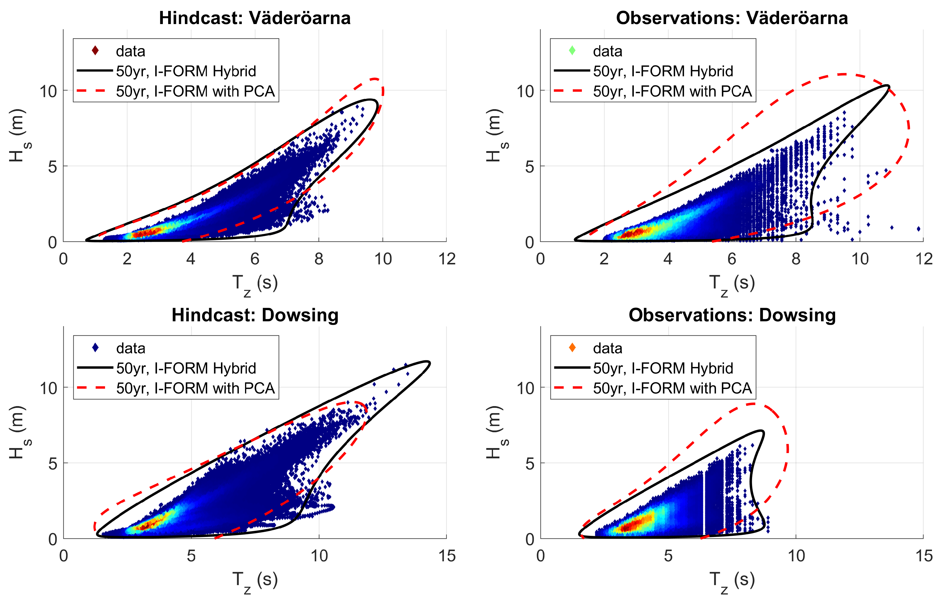
In order to facilitate visualization of the data, the data density approach of Eckert-Gallup et al. [27] was used. Each point in a scatter plot is given a color based on the density of nearby points. To determine the density at a specific point, a circle of radius of 0.15 is considered and the density is simply the number of points in this circle. In the scatter plots, blue means low density and red means high density of points (e.g., Figure 11). In each plot, the color scale is set using the highest data density, which effectively normalizes the density with respect to the total number of points.

2.1. Observations

The observations at Ölands Södra Grund and Väderöarna were obtained from SMHI (Swedish Meteorological and Hydrological Institute) Opendata (https://opendata.smhi.se/). The temporal resolution of the data is 1 h.
For Ölands Södra Grund, data are available during 1978–2004, with 145,982 available measurements which corresponds to a data coverage of 65.5% of the full time span. For Väderöarna, 110,745 measurements during 2005–2019 were used, corresponding to a data coverage of 85.4%.
The observations at Dowsing and Tyne Tees were obtained from WaveNet (www.cefas.co.uk/wavenet), a network of wave buoys located near the UK coastline. WaveNet is operated by Centre for Environment, Fisheries and Aquaculture Science (Cefas). The temporal resolution of the available WaveNet data is 30 min; however, to conform with the other data used in the study, a subset of the available WaveNet data is used which has a temporal resolution of 1 h.
For Tyne Tees, data during 2006–2019 are used, with a total of 95,021 measurements (89.2% data coverage). For Dowsing, the data spans a slightly longer period 2003–2019, with 134,656 measurements (98.5% data coverage).
The wave period used for both the WaveNet and SMHI data is the average zero crossing wave period. In order to determine if a seasonal bias is present in the observations, the data availability was compared for the different months for each data set. It was found that generally the data availability is relatively constant throughout the year, with the most notable exception being Väderöarna where there is a slight reduction during February and March likely due to removal of the wave buoy from the water during risk of icing. Measurement gaps before and after the ice time can potentially impact extreme wave statistics [35].

2.2. Hindcast Data

For the hindcast data, the coastDat-1 data sets are used [36]. They provide hindcast data both for the Baltic Sea [37] and for the Southern North Sea [38]. The spatial resolution of coastDat-1 is about 5.5 km × 5.5 km and the temporal resolution is 1 h. For the Southern North Sea the model data is available for 1958–2007 (50 years) and for the Baltic Sea 1958–2002 (45 years).
The starting point for the coastDat-1 data sets is the NCEP/NCAR Reanalysis [39] which provides gridded global atmospheric data, such as wind and pressure fields. The main steps Weisse et al. [36] used when constructing the hindcast data are displayed in Figure 1. As described in Weisse et al. [36], starting from global atmospheric reanalysis data, the regional atmospheric model REMO [40] was used to obtain a dynamically downscaled wind field with higher spatial resolution.
This high-resolution wind field is then used as input to the wave model WAM [41], using nested grids [36]. At each grid point, WAM represents the current sea state by using a 2D wave spectrum. For each time step, a new 2D wave spectrum is obtained at each grid point by solving a transport equation. By integrating the 2D wave spectrum over all wave directions, one obtains the regular 1D frequency wave spectrum from which wave parameters such as H s and T z can be obtained [42].
For the sites in this study, hindcast data for Ölands Södra Grund and Väderöarna are taken from the coastDat-1 Baltic Sea data set, and for Tyne Tees and Dowsing the coastDat-1 Southern North Sea data set. For the Baltic Sea, the model contains a sea ice component, and for this reason all sea states associated with icing periods were excluded from the analysis in order to only retain ice-free sea states.
Several parameters are available for the coastDat-1 data sets; in this study, the significant wave height and mean zero-crossing period T z were used (in this context, T z is also referred to as T m 02 or similar, see, e.g., in [43]). It should be noted that T z can be hard to estimate as it may be sensitive to high-frequency noise [42]. A known issue of the coastDat-1 data sets is possibility of overestimation of the highest waves in shallow areas [36]. This highlights the importance of comparing environmental contours obtained for both hindcast data and measurement data, as is done in this study for four study sites.
The hindcast data span well beyond 30 years, which allows for long-term analysis of wave parameters [44]. For this reason, a simple linear regression was used on H s to investigate the linear trend in the hindcast data for the four sites. It was found that the trends were relatively small: +1.9 mm/year at Ölands Södra Grund, +3.5 mm/year at Väderöarna, +0.85 mm/year at Tyne Tees, and +1.4 mm/year at Dowsing. Note that trends in reanalysis data (which can translate into trends for hindcast data) may be due to changes in the global observing network and not actual climate trends [45].
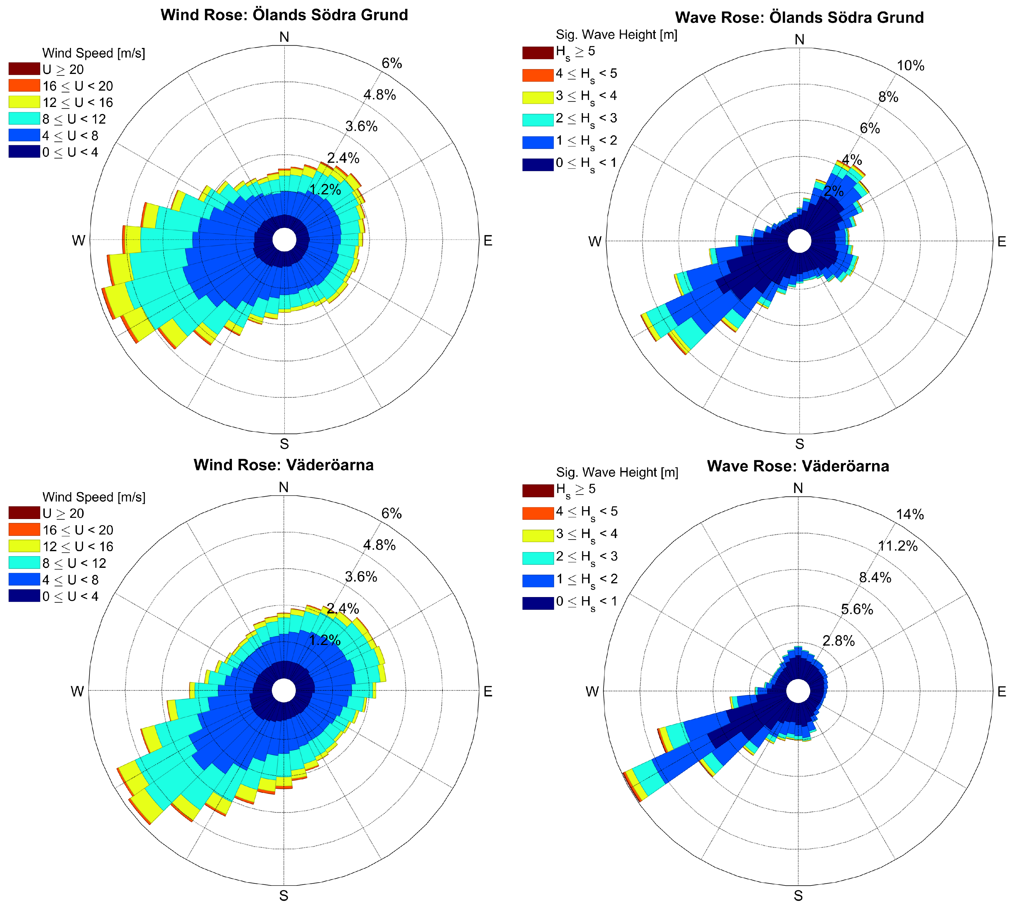
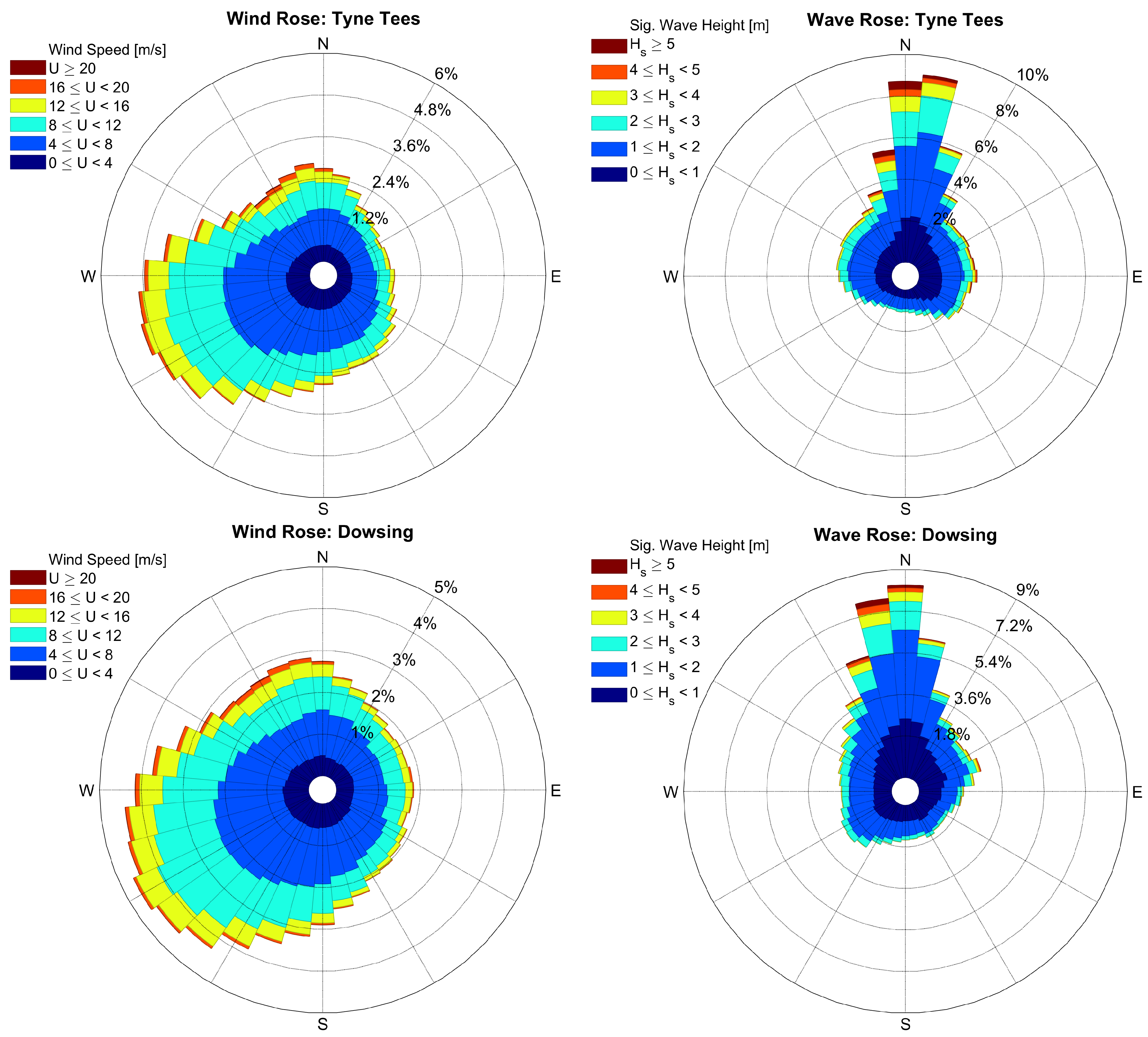
For each site, wind and wave roses were produced in order to obtain a better understanding of the wind and wave climate. Data from coastDat-1 was used. The wind rose consists of the 10-m wind speed and wind direction, and the wave rose consists of H s and wave direction. Figure 3 shows the wind and wave roses for Ölands Södra Grund and Väderöarna, and Figure 4 shows the corresponding roses for Tyne Tees and Dowsing. It is seen for Ölands Södra Grund and Väderöarna that the dominant wind direction is similar to the dominant wave direction. This is not the case for Tyne Tees and Dowsing, which indicates a more complicated wave climate, e.g., due to swell waves, shape of the coastline, etc. More specifically, at Ölands Södra Grund and Väderöarna the wind and wave direction differed by most 30° during 79% and 74% of the time, respectively. At Tyne Tees and Dowsing the corresponding numbers were 52% and 62%, which again indicates a more complicated wave climate for these two sites.
For the hindcast data, the wave age was investigated. It is computed as the phase speed divided by the 10 meter wind speed, and if the wave age exceeds 1.2, it is expected that the sea state predominantly consists of swell waves, see, e.g., Semedo [46]. For Dowsing and Tyne Tees, 26% and 31%, respectively, of the sea states had a wave age above 1.2. For the Ölands Södra Grund and Väderöarna, the corresponding numbers were 14% and 18%. Thus, the wave climate at Dowsing and Tyne Tees has a larger swell wave component than that of Ölands Södra Grund and Väderöarna.

3. Methods

3.1. I-FORM

The inverse first-order reliability method (I-FORM) is described, e.g., in Berg [24] and is briefly outlined here. The method was first proposed by Winterstein et al. [19]. The joint probability distribution of H s and T z is modeled using a conditional approach [6] [section 3.6.3.4], such that
f H s T z ( h , t ) = f H s ( h ) f T z | H s ( t | h ) .
where the arguments h and t refer to values of H s and T z , respectively. The marginal distribution of H s ( f H s ) can be taken as a three-parameter Weibull distribution, and the distribution of T z conditional on H s ( f T z | H s ), can be taken as a log-normal distribution [24]. It should be noted that there are other generalizations of the regular Weibull distribution then the one given in [24], see, e.g., Nadarajah et al. [47] for a review of one such generalization.
The data is split into bins with respect to H s , in this paper a bin width of Δ H s = 1 m is used. In each bin, a log-normal distribution is fitted and its parameters are determined for that particular bin. A fit is then performed to facilitate interpolation and extrapolation of these parameters; in this study, the fitting functions of DNV [6] [section 3.6.3.4] are used.
After this, a Rosenblatt transformation [20] is performed where the original data ( T z , H s ) are transformed into uncorrelated normal variables (see, e.g., in [48]). In these new coordinates, a contour is constructed by considering a circle of radius β . This contour is then transformed back to the original coordinates ( T z , H s ) . As described by Berg [24], one may inflate β to obtain a more satisfactory environmental contour:
β * = β 1 α 0 2 ,
where α 0 2 typically is taken as 0.10–0.20. The motivation behind this is that without such an inflation, the method may produce contour lines which fails to properly represent the underlying data [27].
Also considered here is a hybrid fit proposed by Haver and Nyhus [49] (see also [26,50]). This hybrid fit consists of a log-normal distribution for H s η , and a (2-parameter) Weibull distribution for H s > η :
f H s ( h ) = 1 2 π b ˜ h exp ln h a ˜ 2 2 b ˜ 2 , for h η d ˜ c ˜ h c ˜ d ˜ 1 exp h c ˜ d ˜ , for h > η .
Here, a ˜ can take on any value and b ˜ , c ˜ , and d ˜ are positive. At the threshold η , both the cumulative distribution function and the probability density function of H s are required to be continuous. In Haver [50], the threshold η is determined as follows. First, fit the log-normal part of Equation (2) to all of the data. Due to the continuity constraints, once η is chosen the parameters of the Weibull tail are fixed. By testing different values of η , the value of η which provides the best fit according to a χ 2 -type goodness-of-fit metric can be chosen.
In this paper, a slightly different approach was used, where only the upper 10% of the H s data was considered for the goodness-of-fit in the η selection. The motivation behind this is that for the final environmental contour, it is important to achieve a good representation of the sea states with the most extreme values of H s [27]. In order to avoid a goodness-of-fit metric, which requires binning (i.e., to avoid complications due to the arbitrary choice of bin size), the Cramér–von Mises goodness-of-fit was employed instead (see, e.g., in [51]).

3.2. I-FORM with PCA

Eckert-Gallup et al. [27] have proposed an improvement to the regular I-FORM method. The idea is that one transforms the original data ( T z , H s ) into new coordinates ( C 1 , C 2 ) where the data are uncorrelated. Having performed this transformation, the I-FORM is carried out, however, with different probability distributions and fitting functions than the standard approach.
It is important to keep in mind that although the correlation is zero in the new coordinates, there is still the possibility of a dependence, which must be taken into consideration. For the new coordinates, C 1 is chosen as the direction in which the variance is the largest, and orthogonal to this direction is C 2 . The transformation into ( C 1 , C 2 ) is discussed in detail in Eckert-Gallup et al. [27] and will not be shown here.
For C 1 , Eckert-Gallup et al. [27] use the inverse Gaussian distribution and for C 2 conditioned on C 1 a normal distribution is used. In their paper, a special binning technique for C 1 is employed where bins are defined as containing 250 sea state events. In the present study, however, bins of a constant width Δ C 1 = 1 were employed. This is further discussed in Section 4.1.2. Whereas Eckert-Gallup et al. [27] employs a linear fit for the mean value of the normal distribution, in this study a quadratic fit was used instead.

3.3. 2D POT

In the 2-dimensional peaks-over-threshold (2D POT) method, a set of extreme events are selected by only considering events which exceed thresholds of two variables. Having obtained this set of extreme events, the joint 2-dimensional probability distribution is modeled which in turn allows an estimation of return level curves to be computed. This paper follows closely the methodology of Mazas and Hamm [52]; however, some modifications are required, as they consider compound flooding caused by waves and sea level variation.
The two variables considered here are H s and steepness s, defined as s = H s / L , where L is the wavelength. The wavelength can be obtained from the dispersion relationship (see, e.g., in [42])
L = g T z 2 2 π tanh 2 π h L ,
where h is the depth. This is a nonlinear equation for L which must be solved numerically. Recent developments of very accurate approximations to the linear dispersion relationship for gravity waves can also be considered [53,54] to reduce computational cost for some applications. The motivation for considering the steepness is that certain WEC designs may have a response which is quite sensitive to the steepness [11].
A key aspect of this method is choosing the threshold. A central issue common in POT methods is that if the threshold is set too low, many threshold-exceeding events are not too extreme which can lead to bias in the parameter estimation. On the other hand, if the threshold is set too high, the sample size will be small, which can lead to a large sampling uncertainty in the parameter estimation [55].
Several tools are available to facilitate threshold selection, see, e.g., Coles [55]. This study utilizes plots showing how the Generalized Pareto-parameters ( ξ and σ ) [52] vary with threshold choice. It can be shown that ideally ξ should be constant with respect to the threshold, and σ should vary linearly [55].
Once the thresholds are set, a set of independent events are extracted by only considering one event per storm, see, e.g., Mazas and Hamm [52] and de Oliveira et al. [56] for details. In this paper, a sampling function z = H s + 100 s was used to select the “most extreme” event during a storm, which in this case is the event with highest z. The motivation for using a linear sampling function is its simplicity, and also that linear sampling functions have been used for other applications (see, e.g., in [52]). It was found for the various data sets that events simultaneously exceeding high thresholds of H s and s typically had values of H s (in meters) that were around two orders of magnitude larger than s. Thus, a factor of 100 was chosen in z to ensure that roughly equal weight was placed on the two variables in the sampling process as it was not a priori clear that either variable should be given a larger weight. A sampling time of 48 h is chosen to ensure that different events belong to different mid-latitude storms [57]. By this process the final set of extremes should be statistically independent, and as the autocorrelation has been removed/reduced the events are typically referred to as being “decorrelated”.
The joint two-dimensional probability distribution of the extremes is modeled using a copula approach, whereby the distribution is separated into two distinct parts: (1) the marginal distributions for H s and s, and (2) the dependency structure (copula) of H s and s. Following Mazas and Hamm [52] the marginal distributions are modeled using the Generalized Pareto distribution, and the copula is chosen by testing several copula families and choosing the one with the best fit. In this study, the copula families considered are Gauss, Frank, Galambos, Gumbel–Hougaard, Husler–Reiss, and Clayton. Finally, the return level contour is computed using the standard equation for the joint return period [58]. It should be noted that care always has to be taken when interpreting return periods, particularly when dealing with multiple variables and/or nonstationarity [59,60].

4. Results

4.1. Implementing Each Method

4.1.1. I-FORM

A comparison was performed for the I-FORM method using the two different fits for H s described in Section 3.1: the 3-parameter Weibull fit and the hybrid fit (Equation (2)). It was found that the hybrid fit for H s provided a better fit for the high quantiles, which is not surprising considering that the hybrid fit was implemented in a way which emphasized the highest 10% of the waves. As an example, Figure 5 shows the two different fits for H s for the observational and hindcast data for Tyne Tees. It is seen that both fitting functions produced satisfactory fits for the bulk of the data, but the hybrid fit is better at higher quantiles.
For the environmental contours based on the 3-parameter Weibull fit, an inflation of β was performed using α 0 2 = 0.2 in Equation (1) in order to obtain a more conservative contour which better reflected the data, particularly at high H s . No such inflation was performed for the I-FORM with the hybrid fit.
The hybrid fit (see Section 3.1) places special emphasis on sea states with H s above the 90-percentile. A sensitivity analysis was performed with respect to this percentile in order to investigate the impact on the contours. The 50-year I-FORM contours with the hybrid fit were computed for percentiles in the range 80 to 99, and it was found that for percentiles in the range 80 to 95 the impact on the contour was small. For percentiles above 95 it was found that the impact typically was somewhat larger, with the largest difference noted at Ölands Södra Grund: Figure 6 shows the corresponding contours.
For the hindcast data at Ölands Södra Grund, the threshold η was found to decrease with increasing percentiles, leading to changes in the tail of the distribution. It is seen in the figure that increases in percentiles used in the fitting correspond to decreases in the extreme H s -quantiles. The observational data at the same site showed the opposite trend: η increased with increasing percentiles, leading to an increase in the extreme H s -quantiles.

4.1.2. I-FORM with PCA

It was found that the inverse Gaussian distribution provided a satisfactory fit for the C 1 -component for the observations and hindcast data at all stations. However, for the conditional fitting of C 2 , it was generally found that the normal distribution left room for improvement, one reason being that the C 2 data typically exhibited non-zero skewness, making a symmetrical distribution such as the normal distribution not an ideal choice. This is in contrast to the results of Eckert-Gallup et al. [27], where the C 2 data showed a large degree of symmetry. Another difference was that in the present study, the mean of the normal distribution showed a clear quadratic dependence with respect to C 1 , which motivated the use of a quadratic fitting function (see Section 3.2).
It was found that for the standard deviation parameter of the normal distribution used for the conditional fitting for C 2 , the bins with the largest values of C 1 typically produced irregular values. For this reason, bins with less than 50 events were excluded from this fitting procedure.
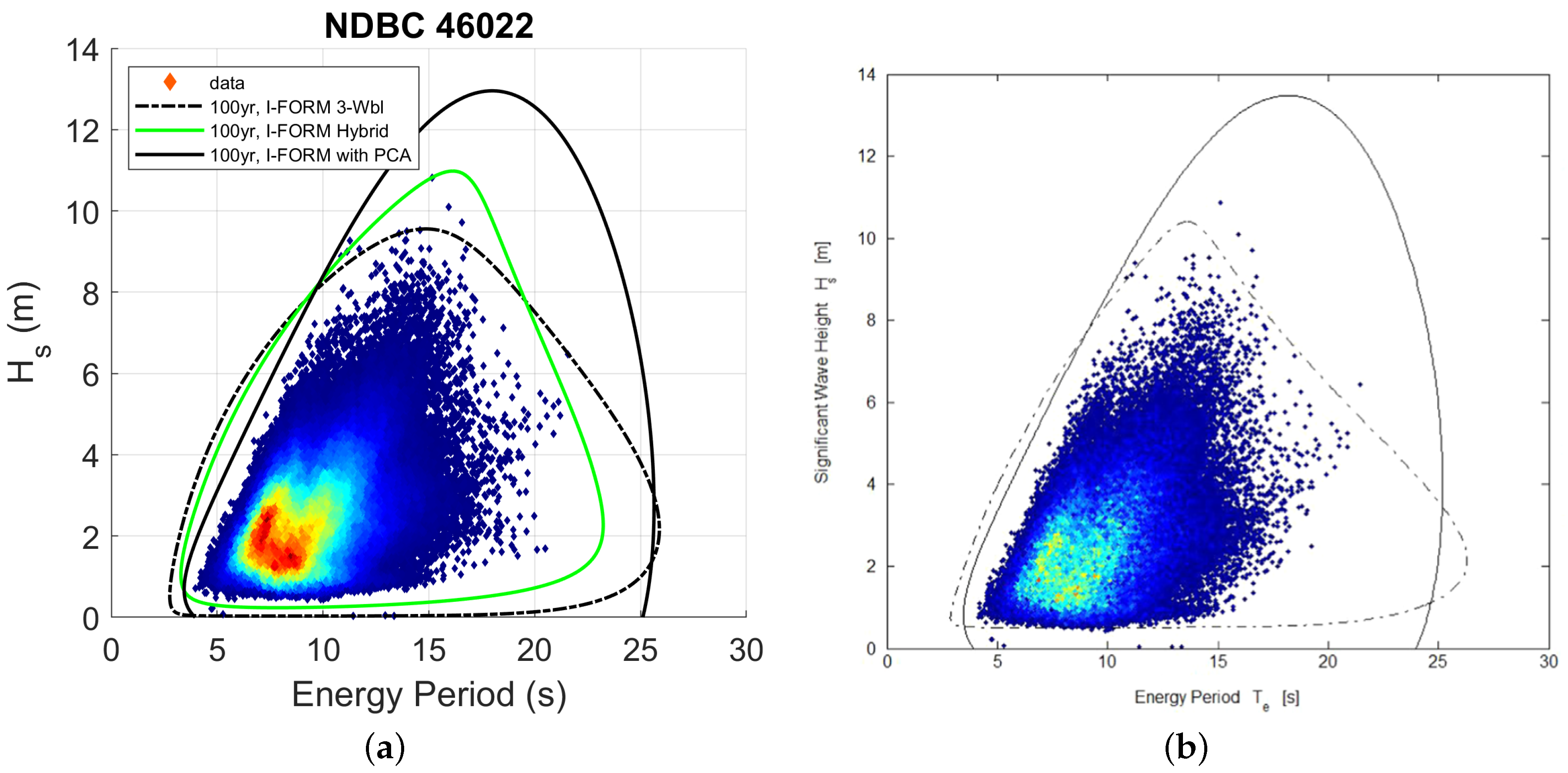
As the binning procedure in this study differs from that of Eckert-Gallup et al. [27], it is not a priori clear that the same results would be obtained for similar data. To investigate this, observations from National Data Buoy Center [61] were used to see if similar results would be obtained for 100-year environmental contours. This buoy, here called “NDBC 46022”, is located outside California, USA. To enable a comparison, the energy period was used and only data from January 1996 to December 2012 were considered. The result is shown in Figure 7a, and it can be confirmed that both the standard I-FORM (with the 3-parameter Weibull) and I-FORM with PCA produced similar 100-year environmental contours as Figure 11b in Eckert-Gallup et al. [27], here reprinted in Figure 7b with permission from Elsevier, Copyright 2016. This similarity is taken as an indication that the binning procedure does not have a major influence on the environmental contours.

4.1.3. 2D POT

Figure 8 shows the implementation of the 2D POT method for the hindcast data at Ölands Södra Grund. In Figure 8a, the original data in the ( T z , H s ) -plane has been transformed to the ( s , H s ) -plane, where s is the steepness. Both thresholds are shown, as are the decorrelated events which are used to estimate the 2D joint probability distribution. The 50-year return level curve has been computed, note that it is only drawn in the region where both thresholds are exceeded. Going back to the ( T z , H s ) -plane, Figure 8b shows the same 50-year return level curve and thresholds.
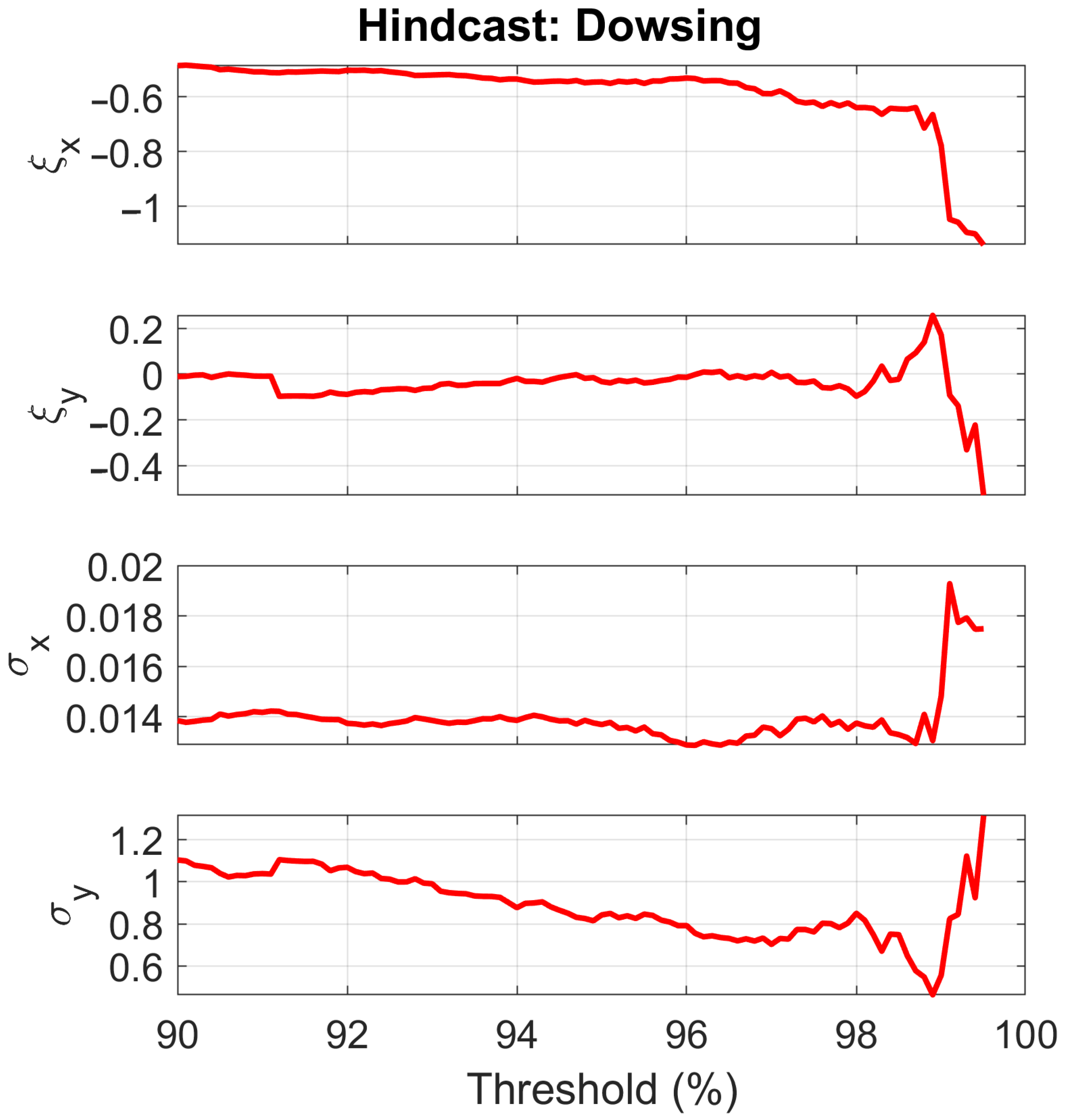
Figure 9 shows the Generalized Pareto parameters as functions of the threshold (see Section 3.3) for the hindcast data at Dowsing. It is seen that ξ for the respective marginal distributions remains relatively constant for thresholds between 92 and 98%, and that the corresponding values of σ are approximately linear in the same threshold range. It was generally found that the threshold choice only had a small impact on the 50-year return level curves, and for simplicity a 95% threshold was selected for both observations and hindcast data at all stations.

4.2. Comparing the Different Data Sets and Different Methods

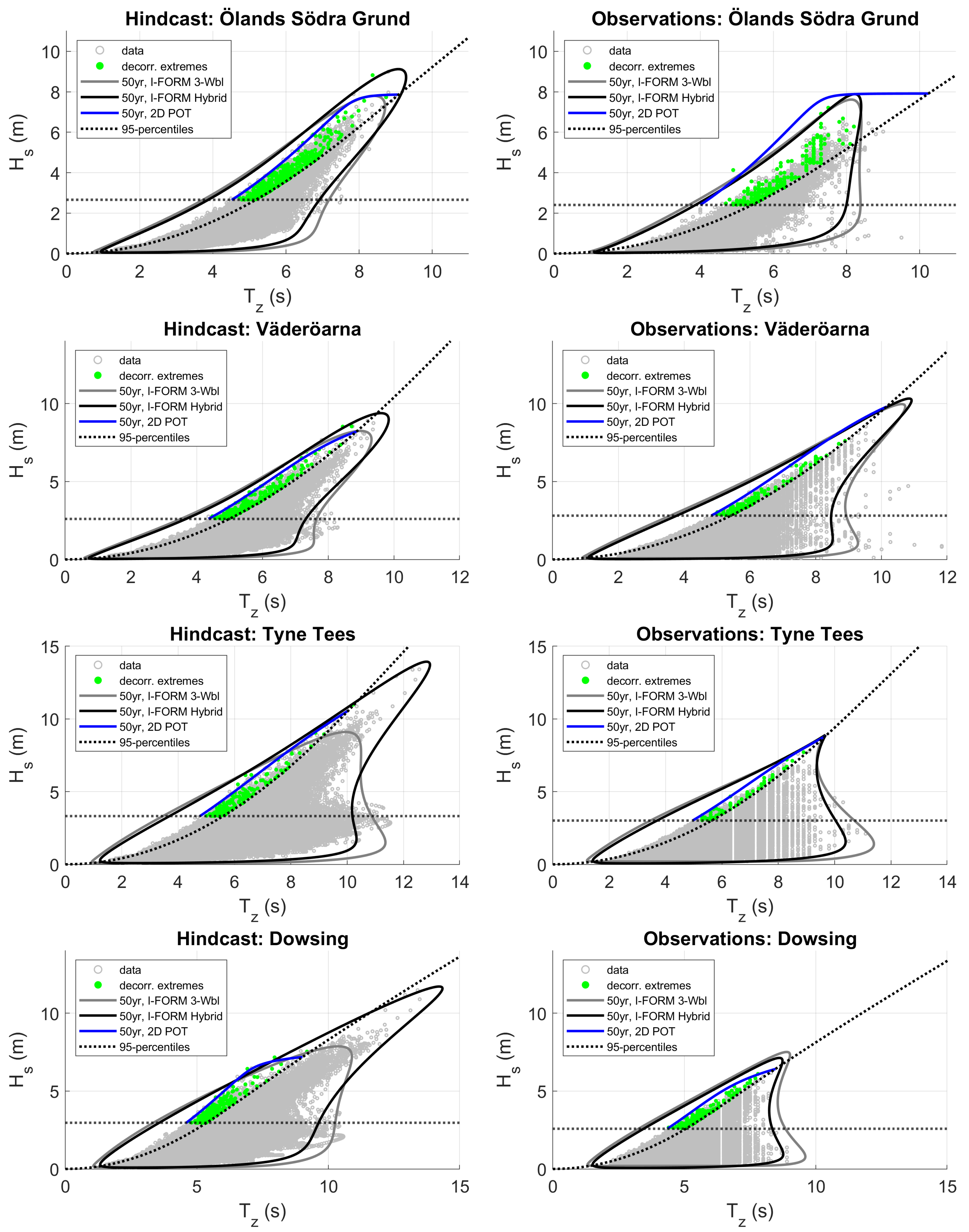
As noted earlier, for the I-FORM the hybrid fit performed better at higher quantiles compared to the 3-parameter Weibull fit (Figure 5). This indicates that for the corresponding environmental contours, the hybrid fit should produce contours which better reflects the data at high H s . This is indeed observed, which shows the importance of using a fit for H s which is able to properly capture the highest waves. Figure 10 shows environmental contours for the two fits. The two different curves differ primarily in how well they reflect the data at high H s , but there is also some difference regarding sea states with high wave period and relatively small H s . For the hindcast data, these latter sea states were found to correspond to sea states with large wave age—above 1.2, i.e., consisting mostly of swell waves (see Section 2.2). It is not surprising that the contours do not properly capture these sea states, as the contours are predominantly based on the wave climate of the bulk of the data (i.e., wind waves).
The 2D POT method is interesting to compare with the various I-FORM methods as it differs fundamentally from such methods in several aspects: (1) it is only based on a subset of the data which only contains extreme events, (2) it only uses statistically independent events from the original data (the autocorrelation has been reduced/removed), and (3) it models the dependency between H s and T z using (2-dimensional) copulas rather than using conditional fitting of 1-dimensional distributions. One obvious drawback of the 2D POT method is that its return levels are only valid above both thresholds, and thus any comparison can only be made in this region of the ( T z , H s ) -plane. However, even in this region the different methods are not expected to match perfectly as there are many different mathematical definitions of return level curves in two dimensions and they typically yield different contours (see, e.g., in [60], and also in [59]). Despite this, it is still interesting to investigate if the different methods yield similar contours.
Figure 10 shows the results from the 2D POT method. It is seen that in many cases, the 2D POT contour is located relatively close to the data, meaning that it gives rise to less conservative 50-year estimates. Keep in mind that for the model data, 45–50 years of data are used to construct the contour and on average one would expect that during this period, circa one (decorrelated) event would exceed this contour. It is seen for the hindcast data that typically more events than expected exceed the 50-year curve obtained from the 2D POT method, indicating that this method tends to underestimate the extreme sea states.
The contours for the I-FORM with PCA are shown in Figure 11 for Väderöarna and Dowsing for both the observations and the hindcast data. Note how the steepness is very large along some parts of the contour for the observations (for a given value of H s , the steepness increases as T z decreases). This method generally performed poorly, especially for the observations, with very large maximum steepness along some contours. This is not surprising as it was noted in Section 4.1.2 that the fitting for C 2 generally did not perform well. It is important to keep in mind that by changing the fitting function for C 2 it is expected that a better fit could be obtained, and thus more sensible environmental contours could be acquired. The main issues with the contours were that the dependency was not properly captured and that the sea states with the highest H s were not reflected by the contour in a reasonable way.
Returning to Figure 7a, it is clear that for this site outside California, USA, the I-FORM with PCA produced a reasonable contour which handled both the dependency between H s and the wave period, as well as the sea states with the highest H s , in a satisfactory manner. It can also be seen in this plot that the I-FORM with the hybrid fit fails to properly enclose the sea states with the highest H s (considering the 17 years of data and the 100-year contour). This highlights that different wave climates may require different methods for estimating environmental contours.
As for comparing the observations and hindcast data for a specific site, care must be taken as the underlying data sets differ in several aspects. One aspect is that observations may have a seasonal bias if some months are overrepresented; however, for the data considered here, it was noted in Section 2.1 that most months generally have similar data availability. Another aspect is that as the environmental contours are based on fewer data for the observations, the sampling error is expected to be larger for such contours. Moreover, the longer the time series, the more extremes are expected to occur.
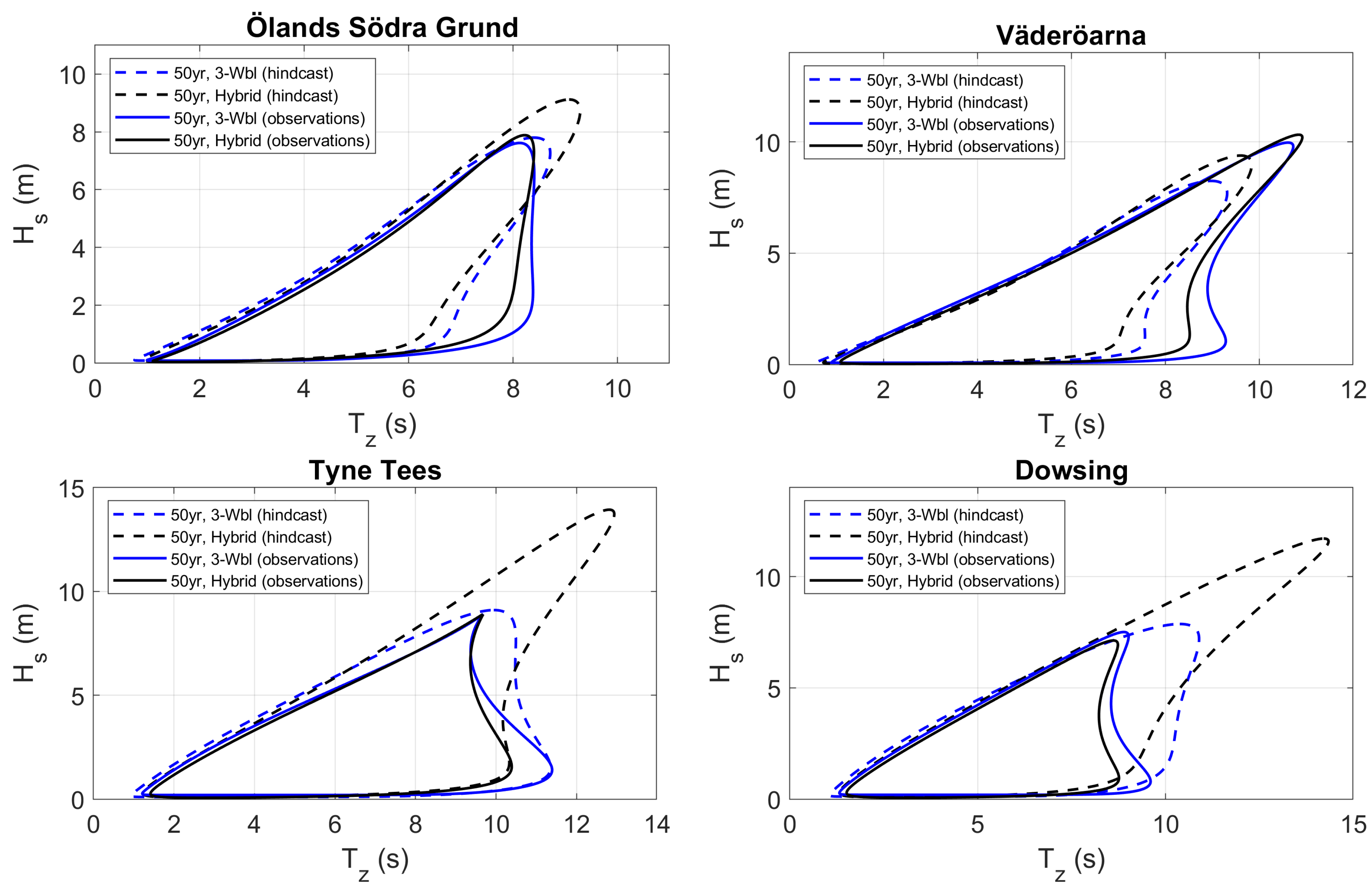
To facilitate comparisons between contours produced by the different data sets, Figure 12 shows the I-FORM contours from both data sets for each of the four sites. It is clear that the agreement between contours for the observations and hindcast data depend both on the site and on the method. It is interesting to note that the more standard I-FORM which uses the three-parameter Weibull fit actually gives comparably more similar contours for the observations and hindcast data at both Tyne Tees and Dowsing. This is likely a reflection of the fact that the bulk of the data is represented reasonably well by the model, and as the sea states with very high H s only have a relatively small impact with this fitting procedure for H s , the final contour is similar for observations and hindcast data (it has been shown that coastDat-1 generally has a good representation of the mean wave parameters [36]).
It is useful to have quantitative measures when comparing different contours, and not solely rely on visual inspection. Table 2 shows a comparison of the contours of Figure 12. The maximum values of H s along each contour are shown for the observations and hindcast data for all sites. For Ölands Södra Grund and Väderöarna the maximum value of H s differs by 1.24 m and 0.94 m, respectively, for the hybrid fit, whereas the same method gives a much larger discrepancy for Tyne Tees and Dowsing. As the hybrid method relies heavily on sea states with high values of H s this result indicates that the hindcast is unable to properly represent such sea states at Tyne Tees and Dowsing potentially related to a higher contribution of swell conditions.
Also shown in Table 2 is the conditional maximum of the steepness s. The maximum value of s was conditioned on points along the contour with H s > H s , max / 2 where H s , max is the maximum value of H s for the observations at each site. This corresponds to a value of H s of 3.61 m (Ölands Södra Grund), 4.26 m (Väderöarna), 4.14 m (Tyne Tees), and 3.09 m (Dowsing). The reason for this restriction is that a relatively large steepness was typically observed in the lower left-hand part of the contours and it was deemed more interesting to only compare sea states where H s was relatively large.
At Väderöarna, it is seen that the maximum steepness for each method is very similar when comparing the observations and hindcast data sets. For the other sites, the hindcast data set gives rise to a larger steepness compared to the contour based on the observations.
As the 2D POT method deals with independent events, it is straightforward to calculate the number of independent events that exceed the contour, and compare this to what is statistically expected. Such calculations, although fairly straightforward, are to our knowledge novel for the application of evaluation of probabilities of compound events of high significant wave height and high wave steepness. The calculations were carried out for a range of different return periods, which also gives an idea of how sensitive the 2D POT method is to changes in the return period.
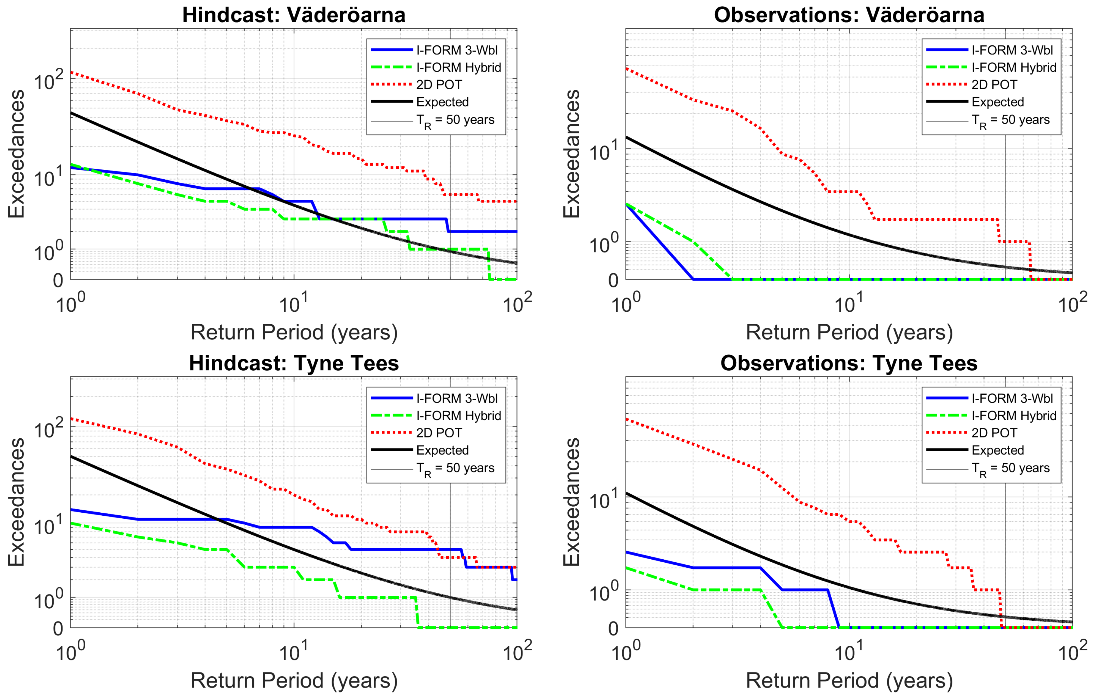
Figure 13 shows the results for Väderöarna and Tyne Tees, both for hindcast data and observations. Return periods from 1 year to 100 years are shown. To avoid difficulties involving plotting 0 in a log scale, a special transformation by Webber [62] was applied to the y-axis which uses a linear scale for the interval [0, 1]. It was found that for all sites and data sets, the 2D POT method consistently underestimated the extreme sea states for most return periods, leading to a larger number of exceedances than what was statistically expected.
Analogous calculations for the I-FORM were carried out in the same region in the ( T z , H s ) -plane using the same independent events. For the I-FORM, it is not a priori clear what the expected number of exceedances is in this region (see e.g., Haselsteiner et al. [60] for more details regarding the probabilistic interpretation of the I-FORM contour). Nevertheless, as this is a region of high importance, it is interesting to investigate the exceedances for the 3-parameter Weibull fit and the hybrid fit for the I-FORM. This is included in Figure 13, and it was found that for the hindcast data at all four sites, the 3-parameter Weibull I-FORM contours generally had more exceedances compared to the corresponding contour with the hybrid fit.
For the 50-year contours for the four hindcast data sets, the 3-parameter Weibull fit led to an average of 3.25 independent exceedances, whereas the corresponding number for the hybrid fit was 1.00. Considering the length of these data sets (45 or 50 years), it can be concluded that the hybrid fit leads to a more reasonable number of independent exceedances. However, this conclusion does not necessarily hold true for lower return periods. In Figure 13, it is, e.g., clear for the hindcast data sets, that the number of exceedances for these two methods has a different scaling with the return period compared to the 2D POT method. This indicates that it may be difficult to draw general conclusions that hold true for all return periods. For the observational data the limited data availability made it difficult to draw any conclusions for the I-FORM using such plots.

5. Discussion

For our study sites it is clear that relatively large differences in contour properties (e.g., Figure 12 and Table 2) can occur depending on whether observations or hindcast data is used, as well as contour method. This is particularly true for Tyne Tees and Dowsing, i.e., the sites which displayed the more complicated wave climate, as was noted in Section 2.2, with, e.g., more swell waves and a larger difference between wind and wave directions.
Visual inspection was found to be practical for comparing contours, but the quantitative comparison of the steepness (in Table 2) is hard to infer from visual means alone and provided insight into how the various data sets and methods differ. Additionally, the plots showing the number of independent sea states that exceeded the different contours provided information not only about the performance of the 50-year contours, but for return periods spanning a larger interval (Figure 13). This is useful as it is not a priori clear how sensitive a contour method is with regards to the chosen return period, and different applications call for different return periods. Being a statistical tool, it is important to keep in mind that one expects more accurate and robust results as more samples are gathered, and that one should not draw too general conclusions from a limited statistical sample.
It is critical neither to underestimate nor overestimate the characteristic load that will be used in designing the WEC. When using a contour method which places large weight on the extremes—such as the hybrid method—then those extremes must be reliable. If not, the end result is a contour which is unreliable which may still fit the data very well. If both observations and hindcast data are available, a bias correction may be applied to the hindcast data to make it more similar to the observations, see, e.g., in [63]. Recall that (Section 2.2) the coastDat-1 hindcasts have been reported to overestimate extreme waves in shallow areas, which may account for some of the discrepancies between the contours.
It should be noted that if there is a clear nonstationarity in the data—for example, if climate change has a strong impact on the wave climate at a particular location, then the idea of return levels has to be reconsidered [59,64]. The lifetime that an offshore structure is designed for also plays a role in determining the importance of investigating—and possibly accounting for—nonstationarity in the data. In the present study, it was noted that the hindcast data displayed linear trends in H s that were relatively small, which provides some justification for using a stationary approach. A possible line of future research might be to perform a more formal analysis of the degree of nonstationarity using, e.g., the nonparametric Mann–Kendall test and also considering additional wave parameters such as the wave period or high monthly percentiles of H s (see, e.g., in [65,66]).
It is clear that in theory, applying PCA could be very advantageous as (1) the linear correlation is removed and (2) the new coordinates single out the most important direction with respect to the variance of the original data set. However, for our study sites, it was found that the fitting procedure of Eckert-Gallup et al. [27] did not work as well as hoped, as it generally led to environmental contours which did not properly represent the data. A remedy would be to try different families of probability distributions, and investigate how this changes the goodness-of-fit as well as the contour itself. Another line of attack would be to use a nonparametric approach, e.g., as suggested in Eckert-Gallup and Martin [67]. Improving the PCA approach for these data sets is one possible topic for future research.
Although the I-FORM method is commonly used and straightforward to implement, it can be hard to interpret and understand the resulting contours from a statistical point of view. As is illustrated in Haselsteiner et al. [60], in the I-FORM method the probability density is not constant along the contour, which makes it difficult to understand what the enclosed region represents.
DNV-RP-C205 [6] [section 3.6.2.3] notes that when modeling the marginal distribution of H s , the POT method should be used with caution as the threshold selection may affect the results. In the present study, the POT method was applied in two dimensions. Here, the main limitation for the application of selecting design conditions was not the threshold selection, but rather the limited region of applicability in the ( T z , H s ) -plane (i.e., above both thresholds). The 2D POT method is more readily suited towards applications where the only area of interest is above the two thresholds, as is common when studying, e.g., the compound nature of certain types of flooding. For example, Bevacqua et al. [58] applied a 2D POT methodology using the variables sea level and precipitation to study compound flooding.
The main appeal of the 2D POT method is that a wide range of available copulas can be used which allows for the modeling of different types of dependency structures. Drawbacks such as threshold selection and obtaining a set of independent events can make such an approach difficult, and other methods may be preferred. In a review of compound extremes in hydrology and meteorology, Hao et al. [68] highlights that several methods are available for the study of events where several variables need to be taken into account, e.g., methods based on quantile regression and various extremeness indicators.
In this study, visual inspection as well as maximum values of scalar quantities (Table 2) were used to compare different contours. Another method which could be employed for such comparison is a measure of goodness-of-fit for the bivariate distribution of H s and T z (see, e.g., in [52]). An issue with such an approach is that for extreme events, one is typically more interested in the regions of low probability, as this is the region where, e.g., the 50-year contours would be located. Restricting attention to this part of the distribution or using a weighting to increase the relative importance of such regions are possible approaches when implementing a relevant goodness-of-fit measure. It is not clear what the best way is to implement such a scheme and no such approach was used in this study, while keeping in mind the limitations of visual inspection.

6. Conclusions

In this study, a comparison was made between 50-year environmental contours for observations and hindcast (model) data. Moreover, different methods for estimating the contours were studied and compared. The comparison was made using visual inspection and also by considering the maximum H s and steepness along the contours. Four sites were considered: one in the Baltic Sea, one in Skagerrak, and two sites in the North Sea.
As for the different methods, it was found that the standard I-FORM method [19] with a hybrid fit for H s [49] generally provided a satisfactory environmental contour which was able to account for the sea states with the highest H s . In this paper, a slight modification was introduced for the hybrid fit where only the highest 10% of the sea states were considered for the threshold selection in order to ensure that the sea states with the highest H s were properly represented by the I-FORM. A sensitivity analysis was performed and it was found that the contours were robust with respect to the choice of using the highest 10% of the sea states: using the highest 5–20% produced nearly identical contours for the four sites under investigation.
For Ölands Södra Grund and Väderöarna, it was found that the observations and hindcast data both produced reasonably similar contours; however, the maximum value of H s did not generally agree (Figure 12 and Table 2). For Tyne Tees and Dowsing, the two sites in the North Sea, the hindcast data tended to overestimate the sea states with high H s , resulting in quite different contours for the highest values of H s for the I-FORM with the hybrid fit. If one instead considered the more traditional I-FORM with a three-parameter Weibull fit for H s , the maximum H s along the contours for observations and hindcast data were similar for Tyne Tees and Dowsing. This is an indication that the bulk of the data is represented reasonably well by the model at these two locations, whereas the extremes (high H s ) are not, which is a known issue for this hindcast data [36]. As noted in Section 1, Neary et al. [30] reported, on the other hand, a hindcast underestimation of sea states with high H s along the environmental contours for their study sites. However, differences in wave climate, hindcast models, and contour method makes a direct comparison difficult.
A 2D POT method was applied by considering high thresholds of H s and steepness s, and using copulas to construct 50-year return level contours. The contours were then transformed to the original variables which allowed for a comparison with other methods. It was found that the 2D POT method tended to underestimate the extreme sea states, and produced less conservative estimates compared to the other methods. This underestimation was found to be consistent for a range of return periods for the different data sets. Despite the limited region of applicability in the ( T z , H s ) -plane, such a comparison is still interesting considering the popularity of the 2D POT method in the study of compound events.
To summarize, care must be taken both in choosing the data and the contour method. Unreliable data inevitably leads to unreliable contours, and contour methods that work well in some wave climates need not work well in others. There is some indication from this work that sites with a larger proportion of swell waves compared to wind waves are more difficult for obtaining reliable contours, but more research into this topic is needed. The environmental contour approach was here examined to determine environmental cases for evaluation of the characteristic design load. This constitutes an important stepping stone in a methodological and modeling chain (Figure 1) aspiring to further develop wave energy converter design.
The pursuit of methods to assess, characterize, and utilize alternative renewable energy sources remains an overarching goal for the scientific community. To meet future energy demands, and simultaneously meet long-term climate goals, renewable energy sources are needed, and the oceans store a significant part of the global energy resources [69].

Author Contributions

Conceptualization, L.W., E.K., E.N., A.R., J.R., and M.G.; methodology, L.W., E.K., and J.R.; software, L.W. and E.K.; validation, L.W. and E.K.; formal analysis, L.W. and E.K.; investigation, L.W. and E.K.; resources, L.W.; data curation, L.W.; writing—original draft preparation, L.W. and E.K.; writing—review and editing, L.W., E.K., E.N., A.R., J.R., and M.G.; visualization, L.W.; supervision, E.N., A.R., and M.G.; project administration, E.N., A.R., and M.G.; funding acquisition, A.R. and M.G. All authors have read and agreed to the published version of the manuscript.

Funding

This research was funded by the Swedish Research Council FORMAS (Grant No. 2018-01784) and the Centre of Natural Hazards and Disaster Science (CNDS). E.K. were partly funded by the Swedish Research Council (VR, Grant No. 2015-04657), the Swedish Energy Authority (Project No. 47264-1) and the Onassis Foundation (Scholarship ID: FZP 021-1/2019-2020).

Institutional Review Board Statement

Not applicable.

Informed Consent Statement

Not applicable.

Data Availability Statement

Publicly available datasets were analyzed in this study. The observational data from SMHI (Swedish Meteorological and Hydrological Institute) Opendata was found here: https://opendata.smhi.se/. The observational data from WaveNet was found here: www.cefas.co.uk/wavenet. The observational data from National Data Buoy Center was found here: https://www.ndbc.noaa.gov/station_page.php?station=46022. The hindcast datasets were found here: http://coastdat.wdc-climate.de/.

Acknowledgments

Ralf Weisse is acknowledged for providing access to the coastDat-1 hindcast data sets.

Conflicts of Interest

The authors declare no conflict of interest. The funders had no role in the design of the study; in the collection, analyses, or interpretation of data; in the writing of the manuscript; or in the decision to publish the results.

References

  1. Coe, R.G.; Neary, V.S.; Lawson, M.J.; Yu, Y.; Weber, J. Extreme Conditions Modeling Workshop Report; Technical Report; National Renewable Energy Lab.(NREL): Golden, CO, USA, 2014.
  2. Czech, B.; Bauer, P. Wave Energy Converter Concepts: Design Challenges and Classification. IEEE Ind. Electron. Mag. 2012, 6, 4–16. [Google Scholar] [CrossRef]
  3. Wolfram, J. On Assessing the Reliability and Availability of Marine Energy Converters: The Problems of a New Technology. Proc. Inst. Mech. Eng. Part O J. Risk Reliab. 2006, 220, 55–68. [Google Scholar] [CrossRef]
  4. International Electrotechnical Commission. IEC TS 62600-2:2019, Technical Repor. 2019. Available online: https://webstore.iec.ch/publication/62399 (accessed on 12 May 2020).
  5. NORSOK Standard. Actions and Action Effects, 2nd ed.; Technical Report N-003; Standards Norway: Lysaker, Norway, 2007. [Google Scholar]
  6. DNV. Environmental conditions and environmental loads. In Recommend Practice DNV-RP-C205; Det Norske Veritas: Hovik, Norway, 2010. [Google Scholar]
  7. Ransley, E.J. Survivability of Wave Energy Converter and Mooring Coupled System Using CFD. Ph.D. Thesis, Plymouth University, England, UK, 2015. [Google Scholar]
  8. Yu, Y.H.; van Rij, J.; Coe, R.; Lawson, M. Preliminary Wave Energy Converters Extreme Load Analysis. In Proceedings of the 35th International Conference on Ocean, Offshore and Arctic Engineering (OMAE2015), St. John’s, NL, Canada, 19–24 June 2015. [Google Scholar] [CrossRef]
  9. Hann, M.; Greaves, D.; Raby, A. Snatch loading of a single taut moored floating wave energy converter due to focussed wave groups. Ocean Eng. 2015, 96, 258–271. [Google Scholar] [CrossRef] [Green Version]
  10. Göteman, M.; Engström, J.; Eriksson, M.; Leijon, M.; Hann, M.; Ransley, E.; Greaves, D. Wave loads on a point-absorbing wave energy device in extreme waves. J. Ocean Wind Energy 2015, 2, 176–181. [Google Scholar] [CrossRef]
  11. Coe, R.G.; Neary, V.S. Review of Methods for Modeling Wave Energy Converter Survival in Extreme Sea States. In Proceedings of the 2nd Marine Energy Technology Symposium (METS2014), Seattle, WA, USA, 15–17 April 2014. [Google Scholar]
  12. Mackay, E. Return Periods of Extreme Loads on Wave Energy Converters. In Proceedings of the 12th European Wave and Tidal Energy Conference, Cork, Ireland, 27 August–1 September 2017. [Google Scholar]
  13. Hiles, C.E.; Robertson, B.; Buckham, B.J. Extreme wave statistical methods and implications for coastal analyses. Estuar. Coast. Shelf Sci. 2019, 223, 50–60. [Google Scholar] [CrossRef]
  14. Vanem, E.; Bitner-Gregersen, E.M. Alternative environmental contours for marine structural design-a comparison study. J. Offshore Mech. Arct. Eng. 2015, 137. [Google Scholar] [CrossRef]
  15. Baarholm, G.S.; Haver, S.; Økland, O.D. Combining contours of significant wave height and peak period with platform response distributions for predicting design response. Mar. Struct. 2010, 23, 147–163. [Google Scholar] [CrossRef]
  16. Muliawan, M.J.; Gao, Z.; Moan, T. Application of the contour line method for estimating extreme responses in the mooring lines of a two-body floating wave energy converter. J. Offshore Mech. Arct. Eng. 2013, 135, 1–10. [Google Scholar] [CrossRef]
  17. Rendon, E.A.; Manuel, L. Long-term loads for a monopile-supported offshore wind turbine. Wind Energy 2014, 17, 209–223. [Google Scholar] [CrossRef]
  18. Coe, R.G.; Yu, Y.H.; Van Rij, J. A Survey of WEC Reliability, Survival and Design Practices. Energies 2018, 11, 4. [Google Scholar] [CrossRef] [Green Version]
  19. Winterstein, S.R.; Ude, T.C.; Cornell, C.a.; Bjerager, P.; Haver, S. Environmental Parameters for Extreme Response: Inverse Form with Omission Factors. In Proceedings of the Icossar-93, Innsbruck, Austria, 9–13 August 1993; pp. 9–13. [Google Scholar]
  20. Rosenblatt, M. Remarks on a Multivariate Transformation. Ann. Math. Stat. 1952, 23, 470–472. [Google Scholar] [CrossRef]
  21. Silva-González, F.; Heredia-Zavoni, E.; Montes-Iturrizaga, R. Development of environmental contours using Nataf distribution model. Ocean Eng. 2013, 58, 27–34. [Google Scholar] [CrossRef]
  22. Huseby, A.B.; Vanem, E.; Natvig, B. A new approach to environmental contours for ocean engineering applications based on direct Monte Carlo simulations. Ocean Eng. 2013, 60, 124–135. [Google Scholar] [CrossRef]
  23. Huseby, A.B.; Vanem, E.; Natvig, B. Alternative environmental contours for structural reliability analysis. Struct. Saf. 2015, 54, 32–45. [Google Scholar] [CrossRef]
  24. Berg, J. Extreme Ocean Wave Conditions for Northern California Wave Energy Conversion Device; SAND Report SAND2011-9034, Technical Report; US Army Corps of Engineers: Washington, DC, USA, 2011.
  25. Vanem, E. Uncertainties in extreme value modelling of wave data in a climate change perspective. J. Ocean Eng. Mar. Energy 2015, 1, 339–359. [Google Scholar] [CrossRef] [Green Version]
  26. Haver, S.; Winterstein, S.R. Environmental contour lines: A method for estimating long term extremes by a short term analysis. Trans. Soc. Nav. Archit. Mar. Eng. 2009, 116, 116–127. [Google Scholar]
  27. Eckert-Gallup, A.C.; Sallaberry, C.J.; Dallman, A.R.; Neary, V.S. Application of principal component analysis (PCA) and improved joint probability distributions to the inverse first-order reliability method (I-FORM) for predicting extreme sea states. Ocean Eng. 2016, 112, 307–319. [Google Scholar] [CrossRef] [Green Version]
  28. Flocard, F.; Ierodiaconou, D.; Coghlan, I.R. Multi-criteria evaluation of wave energy projects on the south-east Australian coast. Renew. Energy 2016, 99, 80–94. [Google Scholar] [CrossRef]
  29. Nilsson, E.; Wrang, L.; Rutgersson, A.; Dingwell, A.; Strömstedt, E. Assessment of extreme and metocean conditions in the Swedish exclusive economic zone for wave energy. Atmosphere 2020, 11, 229. [Google Scholar] [CrossRef] [Green Version]
  30. Neary, V.S.; Ahn, S.; Seng, B.E.; Allahdadi, M.N.; Wang, T.; Yang, Z.; He, R. Characterization of Extreme Wave Conditions for Wave Energy Converter Design and Project Risk Assessment. J. Mar. Sci. Eng. 2020, 8, 289. [Google Scholar] [CrossRef] [Green Version]
  31. Eckert, A.; Martin, N.; Coe, R.G.; Seng, B.; Stuart, Z.; Morrell, Z. Development of a Comparison Framework for Evaluating Environmental Contours of Extreme Sea States. J. Mar. Sci. Eng. 2021, 9, 16. [Google Scholar] [CrossRef]
  32. Björkqvist, J.V.; Rikka, S.; Alari, V.; Männik, A.; Tuomi, L.; Pettersson, H. Wave height return periods from combined measurement–model data: A Baltic Sea case study. Nat. Hazards Earth Syst. Sci. 2020, 20, 3593–3609. [Google Scholar] [CrossRef]
  33. Ross, E.; Astrup, O.C.; Bitner-Gregersen, E.; Bunn, N.; Feld, G.; Gouldby, B.; Huseby, A.; Liu, Y.; Randell, D.; Vanem, E.; et al. On environmental contours for marine and coastal design. Ocean Eng. 2020, 195, 106194. [Google Scholar] [CrossRef]
  34. Velarde, J.; Vanem, E.; Kramhøft, C.; Sørensen, J.D. Probabilistic analysis of offshore wind turbines under extreme resonant response: Application of environmental contour method. Appl. Ocean Res. 2019, 93, 101947. [Google Scholar] [CrossRef]
  35. Björkqvist, J.V.; Lukas, I.; Alari, V.; van Vledder, G.P.; Hulst, S.; Pettersson, H.; Behrens, A.; Männik, A. Comparing a 41-year model hindcast with decades of wave measurements from the Baltic Sea. Ocean Eng. 2018, 152, 57–71. [Google Scholar] [CrossRef] [Green Version]
  36. Weisse, R.; Gaslikova, L.; Geyer, B.; Groll, N.; Meyer, E. coastDat—Model Data for Science and Industry. Die Küste 81 Model. 2014, 81, 5–18. [Google Scholar]
  37. Weisse, R. coastDat-1 Waves Baltic Sea; World Data Center for Climate (WDCC) at DKRZ: Hamburg, Germany, 2015. [Google Scholar] [CrossRef]
  38. Weisse, R. coastDat-1 Waves North Sea Wave Spectra Hindcast (1948–2007); Helmholtz-Zentrum Geesthacht, Zentrum für Material- und Küstenforschung GmbH: Geesthacht, Germany; World Data Center for Climate (WDCC) at DKRZ: Hamburg, Germany, 2012. [Google Scholar] [CrossRef]
  39. Kalnay, E.; Kanamitsu, M.; Kistler, R.; Collins, W.; Deaven, D.; Gandin, L.; Iredell, M.; Saha, S.; White, G.; Woollen, J.; et al. The NCEP/NCAR 40-year reanalysis project. Bull. Am. Meteorol. Soc. 1996, 77, 437–471. [Google Scholar] [CrossRef] [Green Version]
  40. Jacob, D.; Podzun, R. Sensitivity studies with the regional climate model REMO. Meteorol. Atmos. Phys. 1997, 63, 119–129. [Google Scholar] [CrossRef]
  41. The Wamdi Group. The WAM model—A third generation ocean wave prediction model. J. Phys. Oceanogr. 1988, 18, 1775–1810. [Google Scholar] [CrossRef] [Green Version]
  42. Holthuijsen, L.H. Waves in Oceanic and Coastal Waters; Cambridge University Press: New York, NY, USA, 2007; p. 387. [Google Scholar] [CrossRef]
  43. Sheng, W.; Li, H. A method for energy and resource assessment of waves in finite water depths. Energies 2017, 10, 460. [Google Scholar] [CrossRef] [Green Version]
  44. Shanas, P.R.; Kumar, V.S. Trends in surface wind speed and significant wave height as revealed by ERA-Interim wind wave hindcast in the Central Bay of Bengal. Int. J. Climatol. 2015, 35, 2654–2663. [Google Scholar] [CrossRef]
  45. Bengtsson, L.; Hagemann, S.; Hodges, K.I. Can climate trends be calculated from reanalysis data? J. Geophys. Res. D Atmos. 2004, 109. [Google Scholar] [CrossRef] [Green Version]
  46. Semedo, A. Seasonal variability of wind sea and swell waves climate along the Canary Current: The local wind effect. J. Mar. Sci. Eng. 2018, 6, 28. [Google Scholar] [CrossRef] [Green Version]
  47. Nadarajah, S.; Cordeiro, G.M.; Ortega, E.M. The exponentiated Weibull distribution: A survey. Stat. Pap. 2013, 54, 839–877. [Google Scholar] [CrossRef]
  48. Chang, K.H. Reliability Analysis. In e-Design Computer-Aided Engineering Design; Chang, K.H., Ed.; Academic Press: Boston, MA, USA, 2015; Chapter 10; pp. 523–595. [Google Scholar] [CrossRef]
  49. Haver, S.; Nyhus, K.A. A wave climate description for long term response calculations. In Proceedings of the OMAE’1986, Tokyo, Japan, 13–18 April 1986. [Google Scholar]
  50. Haver, S. On the Prediction of Extreme Wave Crest Heights; Technical Report; Manuscript, Statoil: Stavanger, Norway, 2004. [Google Scholar]
  51. Laio, F. Cramer-von Mises and Anderson-Darling goodness of fit tests for extreme value distributions with unknown parameters. Water Resour. Res. 2004, 40. [Google Scholar] [CrossRef]
  52. Mazas, F.; Hamm, L. An event-based approach for extreme joint probabilities of waves and sea levels. Coast. Eng. 2017, 122, 44–59. [Google Scholar] [CrossRef]
  53. Simarro, G.; Orfila, A. Improved explicit approximation of linear dispersion relationship for gravity waves: Another discussion. Coast. Eng. 2013, 80, 15. [Google Scholar] [CrossRef]
  54. Beji, S. Improved explicit approximation of linear dispersion relationship for gravity waves. Coast. Eng. 2013, 73, 11–12. [Google Scholar] [CrossRef]
  55. Coles, S. An Introduction to Statistical Modeling of Extreme Values; Springer Series in Statistics; Springer: London, UK, 2001. [Google Scholar] [CrossRef]
  56. De Oliveira, M.M.F.; Ebecken, N.F.F.; de Oliveira, J.L.F.; Gilleland, E. Generalized extreme wind speed distributions in South America over the Atlantic Ocean region. Theor. Appl. Climatol. 2011, 104, 377–385. [Google Scholar] [CrossRef] [Green Version]
  57. Aarnes, O.J.; Breivik, Ø.; Reistad, M. Wave Extremes in the northeast Atlantic. J. Clim. 2012, 26. [Google Scholar] [CrossRef] [Green Version]
  58. Bevacqua, E.; Maraun, D.; Vousdoukas, M.I.; Voukouvalas, E.; Vrac, M.; Mentaschi, L.; Widmann, M. Higher probability of compound flooding from precipitation and storm surge in Europe under anthropogenic climate change. Sci. Adv. 2019, 5. [Google Scholar] [CrossRef] [PubMed] [Green Version]
  59. Serinaldi, F. Dismissing return periods! Stoch. Environ. Res. Risk Assess. 2015, 29, 1179–1189. [Google Scholar] [CrossRef] [Green Version]
  60. Haselsteiner, A.F.; Ohlendorf, J.H.; Wosniok, W.; Thoben, K.D. Deriving environmental contours from highest density regions. Coast. Eng. 2017, 123, 42–51. [Google Scholar] [CrossRef]
  61. National Data Buoy Center. Station 46022 (LLNR 500)—Eel River—17NM WSW of Eureka, CA. 2020. Available online: https://www.ndbc.noaa.gov/station_page.php?station=46022 (accessed on 18 May 2020).
  62. Webber, J.B.W. A bi-symmetric log transformation for wide-range data. Meas. Sci. Technol. 2013, 24. [Google Scholar] [CrossRef] [Green Version]
  63. Parker, K.; Hill, D.F. Evaluation of bias correction methods for wave modeling output. Ocean Model. 2017, 110, 52–65. [Google Scholar] [CrossRef]
  64. AghaKouchak, A.; Easterling, D.; Hsu, K.; Schubert, S.; Sorooshian, S. Extremes in a Changing Climate: Detection, Analysis and Uncertainty; Springer: Dordrecht, The Netherlands, 2012; p. 429. [Google Scholar]
  65. Woo, H.J.; Park, K.A. Long-term trend of satellite-observed significant wave height and impact on ecosystem in the East/Japan Sea. Deep Sea Res. Part II Top. Stud. Oceanogr. 2017, 143, 1–14. [Google Scholar] [CrossRef]
  66. Caloiero, T.; Aristodemo, F.; Algieri Ferraro, D. Trend analysis of significant wave height and energy period in southern Italy. Theor. Appl. Climatol. 2019, 138, 917–930. [Google Scholar] [CrossRef]
  67. Eckert-Gallup, A.; Martin, N. Kernel density estimation (KDE) with adaptive bandwidth selection for environmental contours of extreme sea states. In Proceedings of the OCEANS 2016 MTS/IEEE Monterey, OCE 2016, Monterey, CA, USA, 19–23 September 2016. [Google Scholar] [CrossRef]
  68. Hao, Z.; Singh, V.P.; Hao, F. Compound extremes in hydroclimatology: A review. Water 2018, 10, 718. [Google Scholar] [CrossRef] [Green Version]
  69. Owusu, P.A.; Asumadu-Sarkodie, S. A review of renewable energy sources, sustainability issues and climate change mitigation. Cogent Eng. 2016, 3. [Google Scholar] [CrossRef]
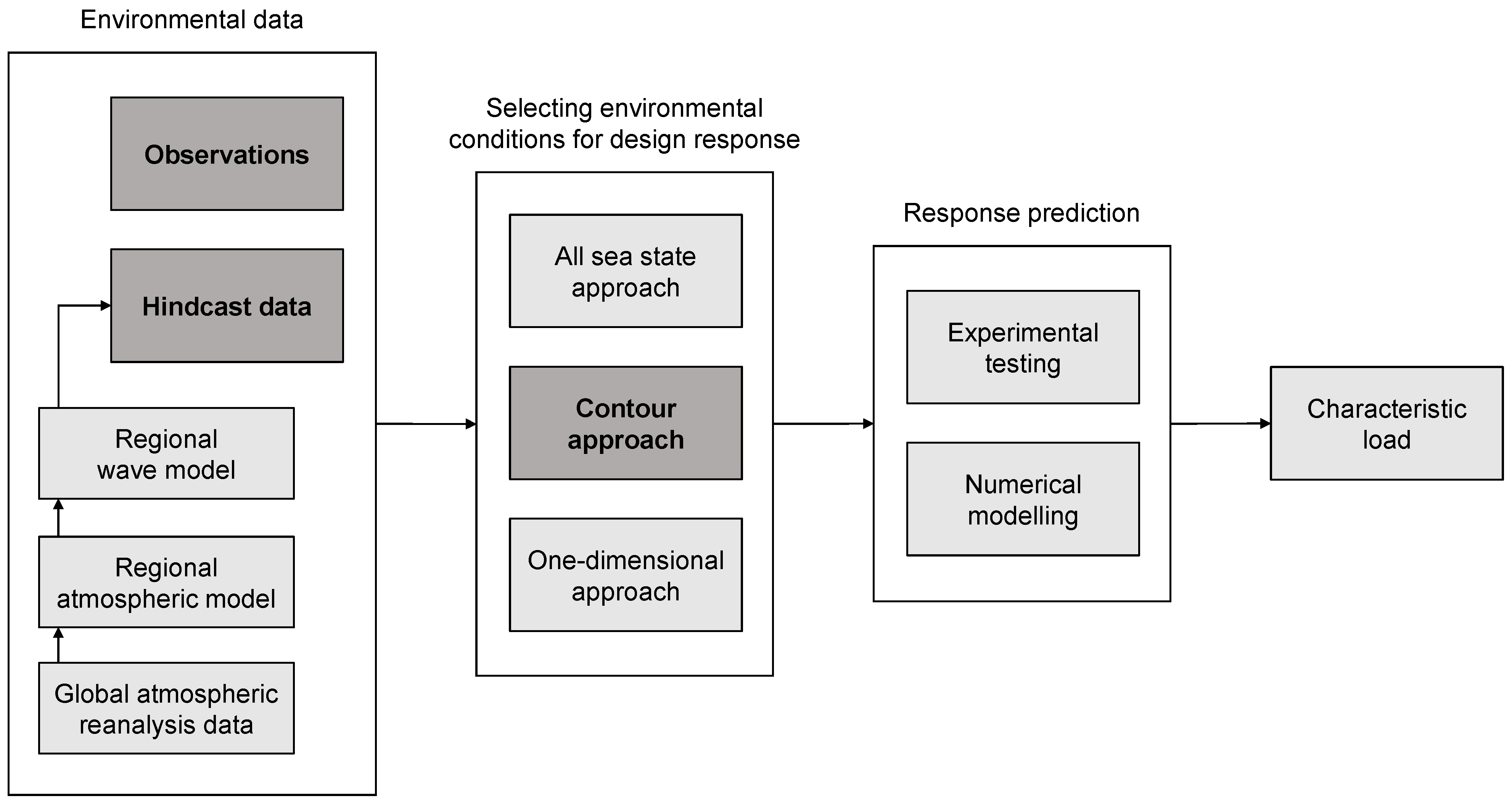
Figure 1. Workflow for determining the characteristic load, with the environmental data as the starting point. The aspects of this workflow that are treated in this paper—observational and hindcast data, and the contour approach—are highlighted.
Jmse 09 00096 g001
Figure 2. The four sites considered in this study.
Jmse 09 00096 g002
Figure 3. Wind and wave roses at Ölands Södra Grund and Väderöarna.
Jmse 09 00096 g003
Figure 4. Wind and wave roses at Tyne Tees and Dowsing.
Jmse 09 00096 g004
Figure 5. Goodness-of-fit plots for H s in the I-FORM method, showing both the 3-parameter Weibull fit (gray dotted line) and the hybrid fit (black dashed line). The hindcast data and observations at Tyne Tees are shown in red in their respective plots. In order to facilitate a comparison for the higher waves, a plot showing only the highest 5% of H s is given for both data sets.
Jmse 09 00096 g005
Figure 6. Sensitivity analysis for the hybrid fit (Equation (2)) for H s in the I-FORM method for 50-year contours. As explained in the text, a percentile of H s is chosen which affects the choice of the threshold η . The region with the largest contour variability is enlarged to more clearly show the colors. Only data from Ölands Södra Grund is shown.
Jmse 09 00096 g006
Figure 7. In subfigure (a) data from NDBC 46022 [61] are used to obtain contours to be compared with Figure 11b in Eckert-Gallup et al. [27], here reprinted in subfigure (b) with permission from Elsevier, Copyright 2016. In the two plots, the black solid lines show the I-FORM with PCA, and the black dashed lines show the I-FORM with 3-parameter Weibull fit for H s . Note that the data density coloring scheme differ slightly for the two plots and thus no comparison regarding data density can be made.
Jmse 09 00096 g007
Figure 8. The 2D Peaks-Over-Threshold method. In subfigure (a), the data are shown in the ( s , H s ) -plane and the 95-percentiles are drawn. The 50-year return level curve is shown in blue. In subfigure (b), the data has been transformed back to the ( T z , H s ) -plane.
Jmse 09 00096 g008
Figure 9. A threshold plot utilized in choosing the thresholds for the 2D POT method. The upper two subplots show how the Generalized Pareto-parameter ξ varies with the choice of threshold for the hindcast data at Dowsing, both for the steepness ( ξ x ) and for the wave height ( ξ y ). Correspondingly the lower two subplots show how the parameter σ varies with threshold.
Jmse 09 00096 g009
Figure 10. Comparing 50-year environmental contours for three different methods: (1) I-FORM with 3-parameter Weibull fit for H s , with β inflated using α 0 2 = 0.2 (gray solid line); (2) I-FORM with a hybrid fit for H s , without inflation (black solid line); and (3) 2D Peaks-Over-Threshold (blue solid line). The threshold percentiles for both H s and the steepness are also shown (black dotted lines).
Jmse 09 00096 g010
Figure 11. Comparing 50-year environmental contours for two methods: (1) I-FORM with a hybrid fit for H s , without inflation (black solid line) and (2) I-FORM with principal component analysis (PCA) (red dashed line).
Jmse 09 00096 g011
Figure 12. Comparing 50-year environmental contours for the observations (solid lines) and the model data (dashed lines). Two methods are shown: (1) I-FORM with 3-parameter Weibull fit for H s , with β inflated using α 0 2 = 0.2 (blue lines) and (2) I-FORM with a hybrid fit for H s , without inflation (black lines).
Jmse 09 00096 g012
Figure 13. Number of independent (decorrelated) sea states which exceed the contour lines in the region above the 95-percentiles of H s and steepness s. Also shown is the expected—in a statistical sense—number of events for the 2D POT method. The return period which is used in this study, 50 years, is highlighted with a vertical gray line.
Jmse 09 00096 g013
Table 1. Properties of the four sites considered in this study. The water depth and the distance to the closest coast are shown. The mean significant wave height is denoted H s ¯ and is given for the observational and hindcast data sets. Also shown is the data availability, in years, for the observations.
SiteLatLonDepth
[m]
Distance
[km]
H s ¯ (obs.)
[m]
H s ¯ (hind.)
[m]
Availability
[years]
Ölands Södra Grund56.0667° N16.6833° E38221.031.0916.7
Väderöarna58.4833° N10.9333° E72181.121.0512.6
Tyne Tees54.9190° N0.7487° W66371.341.5110.8
Dowsing53.5318° N1.0538° E22561.231.3615.4
Table 2. Comparison between the 3-parameter Weibull fit and the hybrid fit (Equation (2)) for the I-FORM method. The maximum value of H s along the 50-year contour is shown. Also shown is the maximum steepness s, conditioned on H s > H s , max / 2 where H s , max is the maximum value of H s for the observations at each site.
Max Hs (m)Cond. max s
SiteData3-WblHybrid3-WblHybrid
Ölands Södra Grundobs.
hind.
7.61
7.80
7.88
9.12
0.099
0.109
0.093
0.103
Väderöarnaobs.
hind.
9.97
8.25
10.32
9.38
0.105
0.104
0.098
0.099
Tyne Teesobs.
hind.
9.07
9.10
10.58
13.94
0.121
0.147
0.112
0.133
Dowsingobs.
hind.
7.51
7.87
7.13
11.71
0.138
0.164
0.125
0.145
Publisher’s Note: MDPI stays neutral with regard to jurisdictional claims in published maps and institutional affiliations.