A Comparison of Decimeter Scale Variations of Physical and Photobiological Parameters in a Late Winter First-Year Sea Ice in Southwest Greenland


Abstract
1. Introduction
2. Materials and Methods
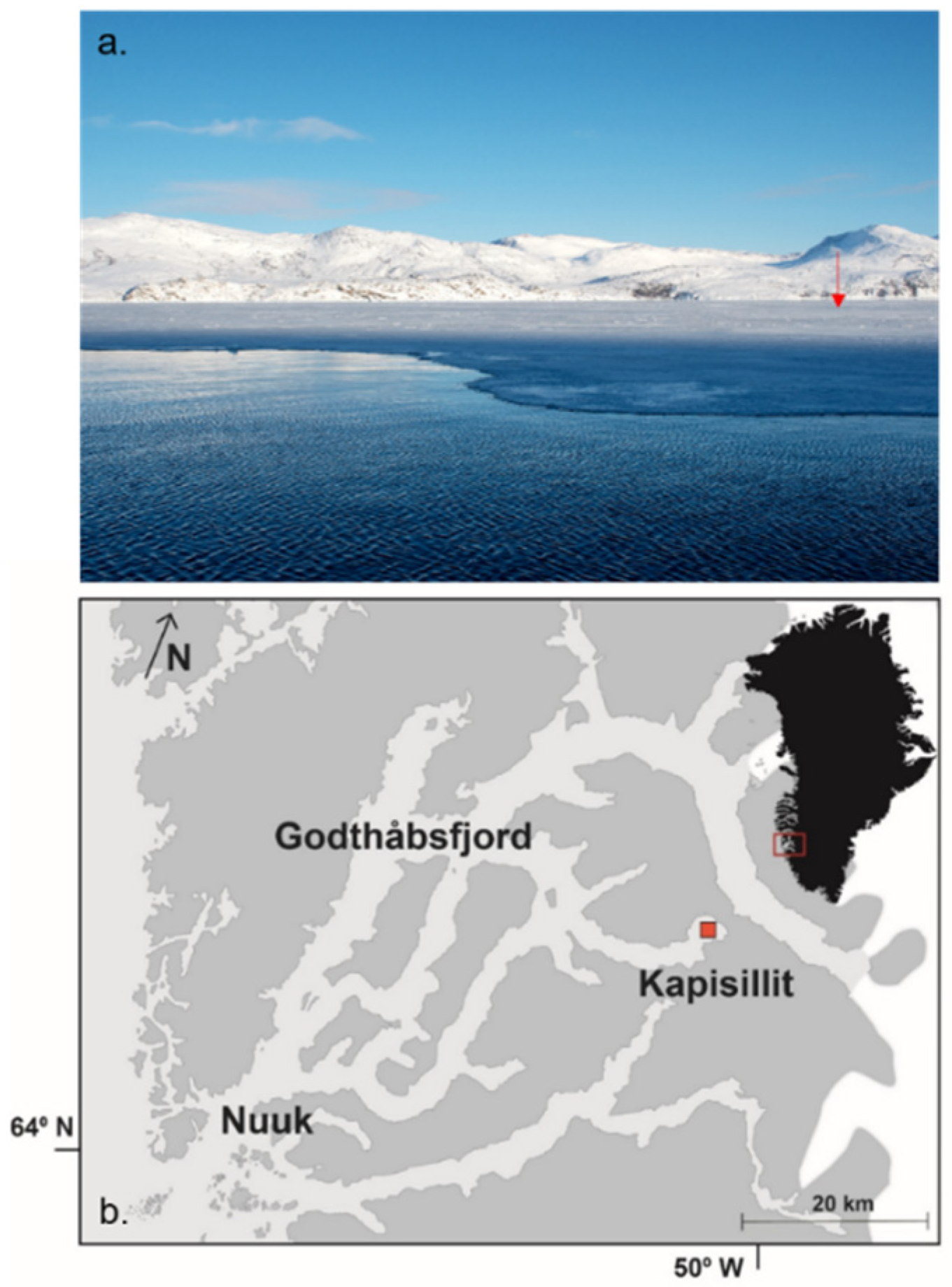
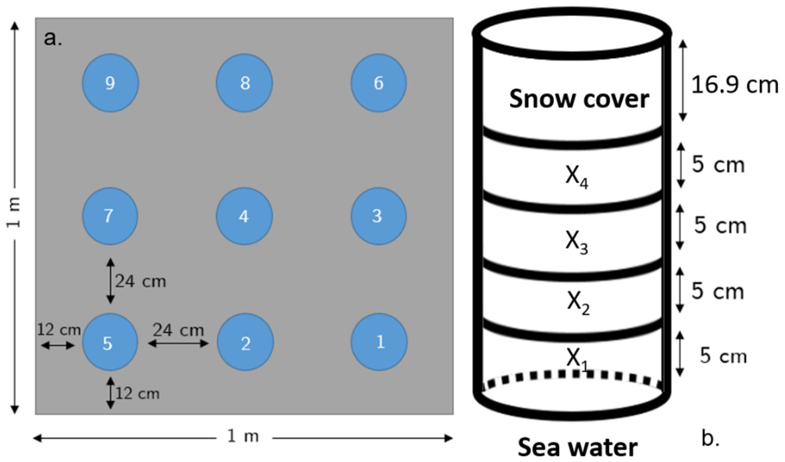
2.1. Study Area and Sampling
2.2. Ice Core Physical Properties
2.3. Chlorophyll Analyses
2.4. Photobiology
2.5. Data Analysis
3. Results
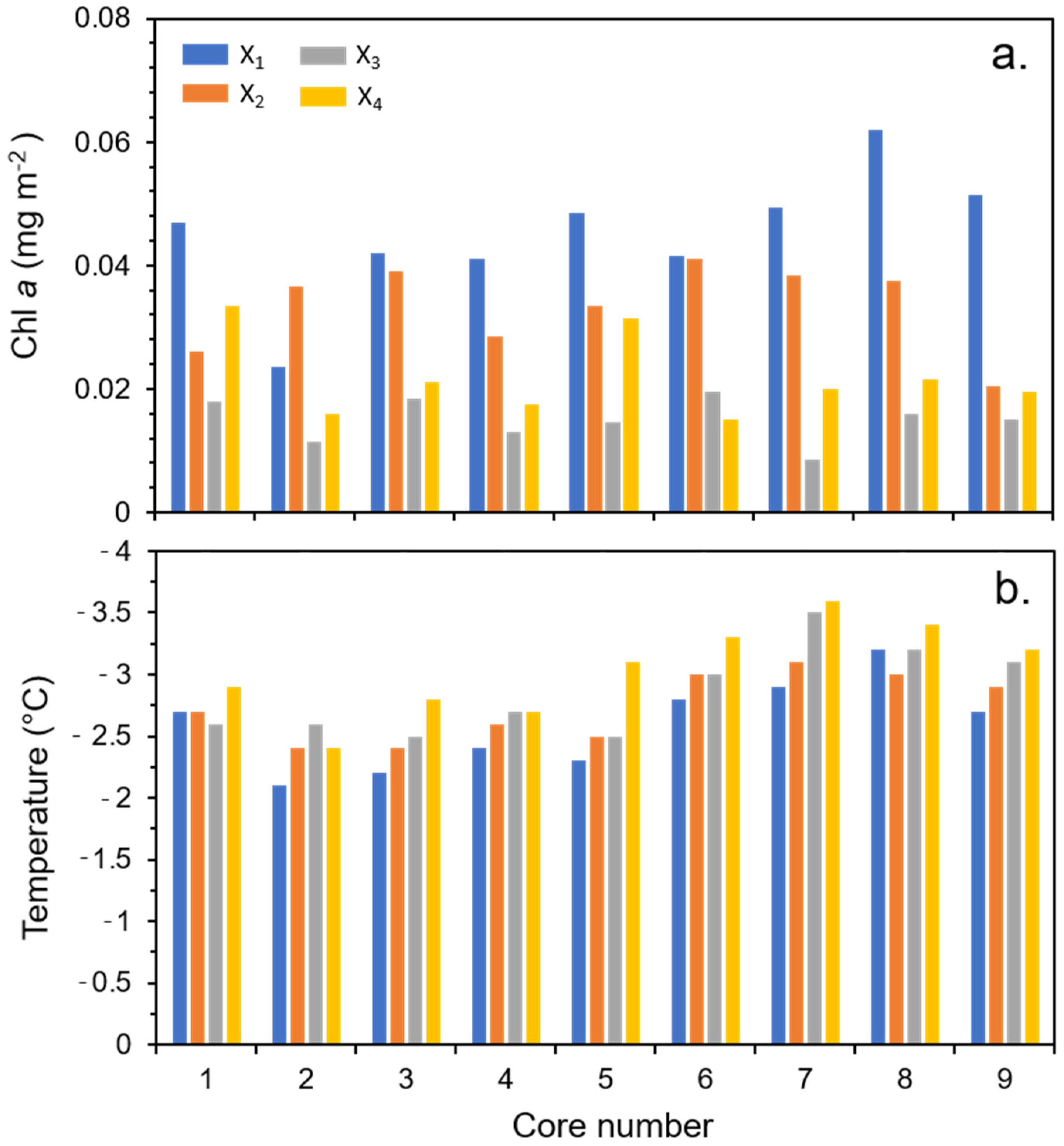
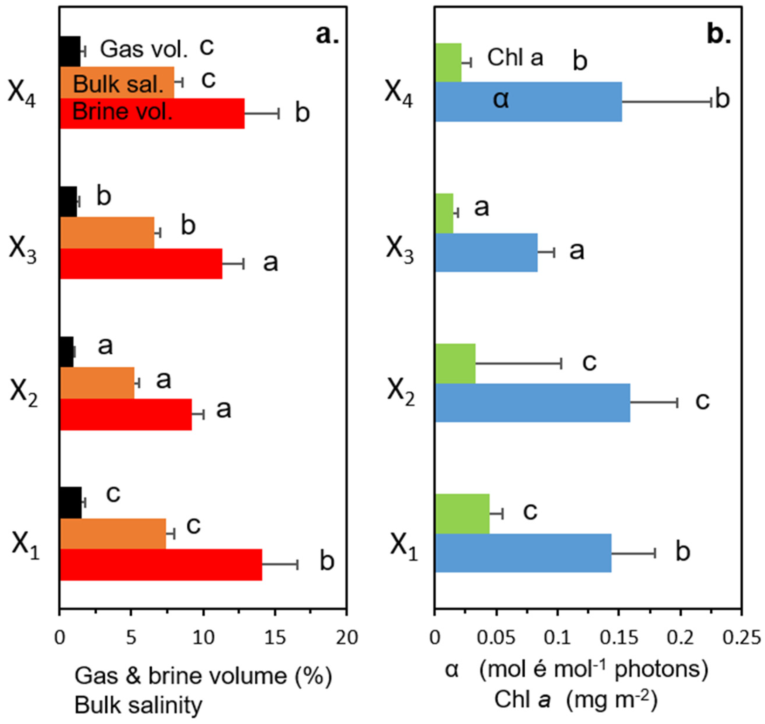
3.1. Physical, Biological, and Photobiological Parameters
3.2. ANOVA Analyses
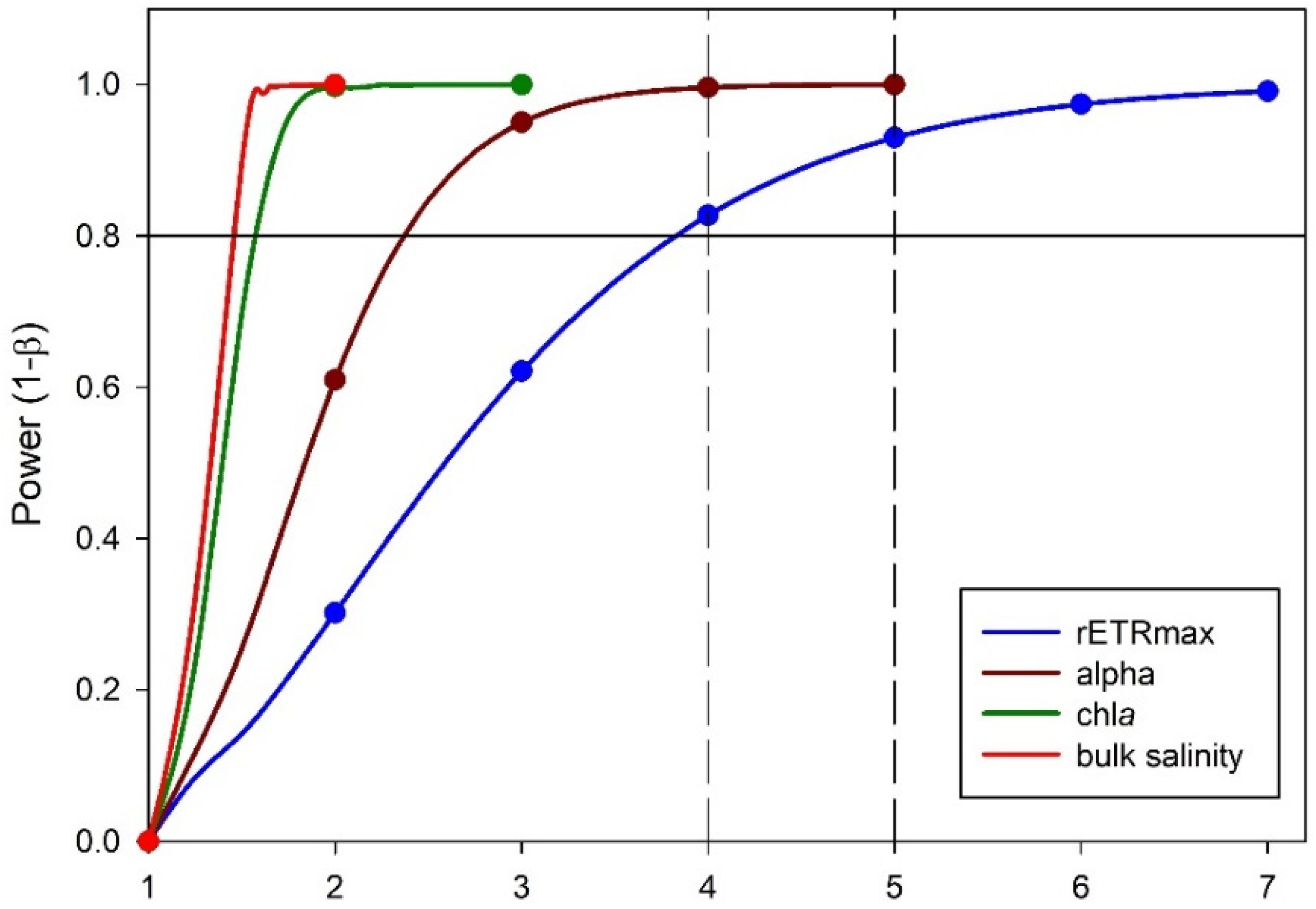
3.3. Power Analysis
4. Discussion
4.1. Kapisillit Data in Comparison
4.2. Variability
5. Conclusions
Author Contributions
Funding
Institutional Review Board Statement
Informed Consent Statement
Data Availability Statement
Acknowledgments
Conflicts of Interest
References
- Parkinson, C.L. Spatially mapped reductions in the length of the Arctic sea ice season. Geophys. Res. Lett. 2014, 41, 4316–4322. [Google Scholar] [CrossRef] [PubMed]
- Parkinson, C.L. A 40-y record reveals gradual Antarctic sea ice increases followed by decreases at rates far exceeding the rates see in the Arctic. Proc. Natl. Acad. Sci. USA 2019, 116, 14414–14423. [Google Scholar] [CrossRef] [PubMed]
- Thackeray, C.W.; Hall, A. An emergent constraint on future Arctic sea-ice albedo feedback. Nat. Clim. Chang. 2019, 9, 972–978. [Google Scholar] [CrossRef]
- Lund-Hansen, L.C.; Hawes, I.; Hancke, K.; Salmansen, N.; Nielsen, J.R.; Balslev, L.; Sorrell, B.K. Effects of increased irradiance and biomass, photobiology, nutritional quality, and pigment composition of Arctic sea ice algae. Mar. Ecol. Prog. Ser. 2020, 648, 95–110. [Google Scholar] [CrossRef]
- Molnár, P.; Bitz, C.M.; Holland, M.M.; Kay, J.E.; Penk, S.R.; Amstrup, S.C. Fasting season length sets temporal limits for global polar bear persistence. Nat. Clim. Chang. 2020, 10, 732–738. [Google Scholar] [CrossRef]
- Kolbach, D.; Schaafsma, F.L.; Graeve, M.; Lebreton, B.; Lange, B.A.; David, C.; Vortkamp, M.; Flores, H. Strong linkage of polar cod (Boreogadus saida) to sea ice algae-produced carbon: Evidence from stomach content, fatty acid and stable isotope analyses. Prog. Oceanogr. 2017, 152, 62–74. [Google Scholar] [CrossRef]
- Lewis, K.M.; Dijken, G.L.; Arrigo, K.R. Changes in phytoplankton concentration now drive increased Arctic Ocean primary production. Science 2020, 369, 198–202. [Google Scholar] [CrossRef]
- Gosselin, M.; Legendre, L.; Therriault, J.-C.; Demers, S.; Rochet, M. Physical control of the horizontal patchiness of the sea-ice microalgae. Mar. Ecol. Prog. Ser. 1986, 29, 289–298. [Google Scholar] [CrossRef]
- Granskog, M.A.; Kaartokallio, H.; Kousa, H.; Thomas, D.N.; Ehn, J.; Sonninen, E. Scales of horizontal patchiness in chlorophyll a, chemical and physical properties of landfast sea ice in the Gulf of Finland (Baltic Sea). Polar Biol. 2005, 28, 276–283. [Google Scholar] [CrossRef]
- Eicken, H.; Lange, M.A.; Dieckmann, G.S. Spatial variability of sea-ice properties in the Northwestern Weddell Sea. J. Geophys. Res. Oceans 1991, 96, C00456. [Google Scholar] [CrossRef]
- Perovich, D.K.; Roesler, C.S.; Pegau, W.S. Variability in Arctic sea ice properties. J. Geophys. Res. Oceans 1998, 103, C01614. [Google Scholar] [CrossRef]
- Rysgaard, S.; Kühl, M.; Glud, R.N.; Hansen, J.W. Biomass, production and horizontal patchiness of sea ice algae in a high-Arctic fjord (Young Sound, NE Greenland). Mar. Ecol. Prog. Ser. 2001, 223, 15–26. [Google Scholar] [CrossRef]
- Cimoli, E.; Meiners, K.M.; Lund-Hansen, L.C.; Lucieer, V. Spatial variability in sea-ice algal biomass: An under-ice remote sensing perspective. Adv. Polar Sci. 2017, 28. [Google Scholar] [CrossRef]
- Cimoli, E.; Lucieer, A.; Meiners, K.; Lund-Hansen, L.C.; Kennedy, F.; Martin, A.; McMinn, A.; Lucieer, V. Towards improved estimates of sea-ice algal biomass: Experimental assessment of hyperspectral imaging cameras for under-ice studies. Ann. Glaciol. 2017, 58, 68–77. [Google Scholar] [CrossRef]
- Lange, B.; Katlein, C.; Castellani, G.; Fernández-Méndez, M.; Nicolaus, N.; Peeken, I.; Flores, H. Characterizing spatial variability of the ice algal chlorophyll a and net primary production between sea ice habitats using the horizontal profiling platforms. Front. Mar. Sci. 2017, 4, 349. [Google Scholar] [CrossRef]
- Meiners, K.M.; Vancoppenolle, M.; Thanassekos, S.; Dieckmann, G.S.; Thomas, D.N.; Tison, J.L.; Arrigo, K.R.; Garrison, D.L.; McMinn, A.; Lannuzel, D.; et al. Chlorophyll a in Antarctic sea ice from historical ice core data. Geophys. Res. Lett. 2012, 39, L21602. [Google Scholar] [CrossRef]
- Søgaard, D.N.; Kristensen, M.; Rysgaard, S.; Glud, R.N.; Hansen, P.J.; Hilligsøe, K.M. Autotrophic and heterotrophic activity in Arctic first-year sea ice: Seasonal study from Malene Bight, SW Greenland. Mar. Ecol. Prog. Ser. 2010, 419, 31–45. [Google Scholar] [CrossRef]
- Søgaard, D.H.; Thomas, D.N.; Rysgaard, S.; Glud, R.N.; Noram, L.; Kaartokallio, H.; Juul-Pedersen, T.; Geilfus, N.-X. The relative contributions of biological and abiotic processes to carbon dynamics in subarctic sea ice. Polar Biol. 2013, 36, 1761–1777. [Google Scholar] [CrossRef]
- Manes, S.S.; Gradinger, R. Small scale vertical gradients of Arctic ice algal photo physiological properties. Photosynth. Res. 2009, 102, 53–66. [Google Scholar] [CrossRef]
- Gradinger, R.; Bluhm, B. Timing of ice algal grazing by the arctic nearshore benthic amphipod Inisimus litoralis. Arctic 2010, 63, 355–358. [Google Scholar] [CrossRef]
- Mundy, C.J.; Ehn, K.; Barber, D.G.; Michel, C. Influence of snow cover and algae on the spectral dependent of transmitted irradiance through Arctic landfast first-year sea ice. J. Geophys. Res. 2007, 112, C03007. [Google Scholar] [CrossRef]
- Lund-Hansen, L.C.; Hawes, I.; Sorrell, B.K.; Nielsen, M.H. Removal of snow cover inhibits spring growth of Arctic ice algae through physiological and behavioral effects. Polar Biol. 2014, 37, 471–481. [Google Scholar] [CrossRef]
- Robineau, B.; Legendre, L.; Kishino, M.; Kudoh, S. Horizontal heterogeneity of microalgal biomass in the first-year sea ice of Saroma-ko Lagoon (Hokkaido, Japan). J. Mar. Syst. 1997, 11, 81–91. [Google Scholar] [CrossRef]
- Steffens, M.; Granskog, M.A.; Kaartokallio, H.; Kousa, H.; Luodekari, K.; Papadimitriou, S.; Thomas, D.N. Spatial variation of biogeochemical properties of landfast sea ice in the Gulf of Bothnia, Baltic Sea. Ann. Glaciol. 2006, 44, 80–87. [Google Scholar] [CrossRef]
- Nicolaus, M.; Katlein, C.; Maslanik, J.; Hendricks, S. Changes in Arctic sea ice result in increasing light transmittance and absorption. Geophys. Res. Lett. 2012, 39. [Google Scholar] [CrossRef]
- Mikkelsen, D.M.; Rysgaard, S.; Glud, R.N. Microalgal composition and primary production in Arctic sea ice: A seasonal study from Kobbefjord (Kangerluarsunnguaq), West Greenland. Mar. Ecol. Prog. Ser. 2008, 368, 65–74. [Google Scholar] [CrossRef]
- Cox, G.F.N.; Weeks, W.F. Equations for determining the gas and brine volumes in sea-ice samples. J. Glaciol. 1983, 29, 306–316. [Google Scholar] [CrossRef]
- Ralph, P.J.; Gademann, R. Rapid light curves: A powerful tool to assess photosynthetic activity. Aquat. Bot. 2005, 82, 222–237. [Google Scholar] [CrossRef]
- Schreiber, U. Photosynthesis: Mechanisms and Effects, V; Garab, G., Ed.; Kluwer Academic Publishers: Dordrecht, The Netherlands, 1998; pp. 4253–4258. [Google Scholar]
- Faul, F.; Erdfelder, E.; Lang, A.-G.; Buchner, A. G*Power 3: A flexible statistical power analysis program for the social, behavioral, and biomedical sciences. Behav. Res. Methods 2007, 39, 175–191. [Google Scholar] [CrossRef]
- Steidl, R.J.; Hayes, J.P.; Schauber, E. Statistical Power Analysis in Wildlife Research. J. Wildl. Manag. 1997, 61, 270–279. Available online: https://www.jstor.org/stable/3802582 (accessed on 11 December 2020). [CrossRef]
- Leu, E.; Mundy, C.J.; Assmy, P.; Campbell, K.; Gabrielsen, T.M.; Gosselin, M.; Juul-Pedersen, T.; Gradinger, R. Arctic spring awekening—Steering principles behind the phenology of vernal ice algal blooms. Prog. Oceanogr. 2015, 139, 151–170. [Google Scholar] [CrossRef]
- Petrich, C.; Eicken, H. Overview of sea ice growth and properties. In Sea Ice, 3rd ed.; Thomas, D.N., Ed.; Wiley Blackwell: Oxford, UK, 2016; 652p. [Google Scholar] [CrossRef]
- Tucker, W.B.; Gow, A.J.; Richter, J.A. On small-scale horizontal variations of salinity in first-year sea ice. J. Geophys. Res. 1984, 89, 6505–6514. [Google Scholar] [CrossRef]
- Hancke, K.; Lund-Hansen, L.C.; Pedersen, S.; King, M.d.; Andersen, P.; Sorrell, B.K. Extreme low light requirement for algae growth underneath sea ice: A case study from Station Nord, NE Greenland. J. Geophys. Res. Oceans 2018, 123, 985–1000. [Google Scholar] [CrossRef]


| Ice Thickness | 20.4 ± 0.7 cm |
| Snow depth | 16.9 ± 0.3 cm |
| Surface PAR | 673.1 ± 49.8 µmol photons m−2 s−1 |
| Transmittance | 0.01 ± 0.001 |
| Albedo | 0.82 ± 0.04 |
| X1 | X2 | X3 | X4 | |
|---|---|---|---|---|
| Temperature (°C) | −2.58 ± 0.36 | −2.73 ± 0.27 | −2.86 ± 0.36 | −3.04 ± 0.38 |
| Bulk Salinity | 7.46 ± 0.57 | 5.18 ± 0.34 | 6.61 ± 0.41 | 8.00 ± 0.57 |
| Brine Density (g cm−3) | 1.04 ± 0.01 | 1.04 ± 0.01 | 1.04 ± 0.01 | 1.04 ± 0.01 |
| Brine Salinity | 45.63 ± 6.09 | 48.07 ± 4.59 | 50.09 ± 5.94 | 53.23 ± 6.27 |
| Brine Volume (%) | 14.16 ± 2.44 | 9.19 ± 0.87 | 11.31 ± 1.54 | 12.91 ± 2.34 |
| Air Volume (%) | 1.57 ± 0.25 | 0.94 ± 0.09 | 1.24 ± 0.16 | 1.49 ± 0.25 |
| Chl a (mg m−2) | 0.045 ± 0.01 | 0.033 ± 0.07 | 0.015 ± 0.004 | 0.022 ± 0.07 |
| ΦPSII_max | 0.31 ± 0.11 | 0.26 ± 0.07 | 0.23 ± 0.08 | 0.24 ± 0.10 |
| α (mol é mol−1 photons) | 0.14 ± 0.04 | 0.16 ± 0.04 | 0.08 ± 0.01 | 0.15± 0.07 |
| rETRmax (µmol é m−2 s−1) | 6.21 ± 3.77 | 4.74 ± 2.80 | 3.79 ± 3.73 | 2.00 ± 0.98 |
| Ek (µmol photon m−2 s−1) | 41.51 ± 19.76 | 39.04 ± 29.56 | 43.22 ± 31.80 | 13.90 ± 3.63 |
| Within-Core Variation | Df * | MS | F | p |
|---|---|---|---|---|
| Temperature (°C) | 3, 32 | 0.335 | 2.81 | 0.055 |
| Bulk salinity | 3, 32 | 13.61 | 58.48 | <0.001 |
| Brine salinity (g cm−3) | 3, 32 | 93.27 | 2.81 | 0.055 |
| Brine volume (%) | 3, 32 | 41.52 | 11.41 | <0.001 |
| Air volume (%) | 3, 32 | 0.72 | 18.52 | <0.001 |
| Chl a (mg m−2) | 3, 32 | 0.403 | 31.5 | <0.001 |
| ΦPSII_max | 3, 23 | 0.025 | 0.924 | 0.455 |
| α (mol é mol−1 photons) | 3, 23 | 0.317 | 2.87 | 0.003 |
| rETRmax (µmol é m−2 s−1) | 3, 23 | 0.101 | 6.05 | 0.059 |
| Ek (µmol photons m−2 s−1) | 3, 23 | 0.258 | 2.54 | 0.082 |
| Between-core variation | ||||
| Temperature (°C) | 8, 27 | 0.419 | 7.73 | <0.001 |
| Bulk salinity | 8, 27 | 0.179 | 0.103 | 0.999 |
| Brine salinity (g cm−3) | 8, 27 | 116.74 | 7.74 | <0.001 |
| Brine volume (%) | 8, 27 | 8.77 | 1.39 | 0.247 |
| Air volume (%) | 8, 27 | 0.078 | 0.76 | 0.644 |
| Chl a (mg m−2) | 8, 27 | 0.015 | 0.273 | 0.969 |
| ΦPSII_max | 8, 18 | 0.03 | 1.21 | 0.348 |
| α (mol é mol−1 photons) | 8, 18 | 0.024 | 0.88 | 0.554 |
| rETRmax (µmol é m−2 s−1) | 8, 18 | 0.14 | 1.07 | 0.428 |
| Ek (µmol photons m−2 s−1) | 8, 18 | 0.133 | 1.165 | 0.371 |
Publisher’s Note: MDPI stays neutral with regard to jurisdictional claims in published maps and institutional affiliations. |
© 2021 by the authors. Licensee MDPI, Basel, Switzerland. This article is an open access article distributed under the terms and conditions of the Creative Commons Attribution (CC BY) license (http://creativecommons.org/licenses/by/4.0/).
Share and Cite
Lund-Hansen, L.C.; Petersen, C.M.; Søgaard, D.H.; Sorrell, B.K. A Comparison of Decimeter Scale Variations of Physical and Photobiological Parameters in a Late Winter First-Year Sea Ice in Southwest Greenland. J. Mar. Sci. Eng. 2021, 9, 60. https://doi.org/10.3390/jmse9010060
Lund-Hansen LC, Petersen CM, Søgaard DH, Sorrell BK. A Comparison of Decimeter Scale Variations of Physical and Photobiological Parameters in a Late Winter First-Year Sea Ice in Southwest Greenland. Journal of Marine Science and Engineering. 2021; 9(1):60. https://doi.org/10.3390/jmse9010060
Chicago/Turabian StyleLund-Hansen, Lars Chresten, Clara Marie Petersen, Dorte Haubjerg Søgaard, and Brian Keith Sorrell. 2021. "A Comparison of Decimeter Scale Variations of Physical and Photobiological Parameters in a Late Winter First-Year Sea Ice in Southwest Greenland" Journal of Marine Science and Engineering 9, no. 1: 60. https://doi.org/10.3390/jmse9010060
APA StyleLund-Hansen, L. C., Petersen, C. M., Søgaard, D. H., & Sorrell, B. K. (2021). A Comparison of Decimeter Scale Variations of Physical and Photobiological Parameters in a Late Winter First-Year Sea Ice in Southwest Greenland. Journal of Marine Science and Engineering, 9(1), 60. https://doi.org/10.3390/jmse9010060