Transfer Learning for Prognostics and Health Management (PHM) of Marine Air Compressors ^†

Abstract

Prognostics is an engineering discipline focused on predicting the time at which a system or a component will no longer perform its intended function. Due to the requirements of system safety and reliability, the correct diagnosis or prognosis of abnormal condition plays a vital role in the maintenance of industrial systems. It is expected that new requirements in regard to autonomous ships will push suppliers of maritime equipment to provide more insight into the conditions of their systems. One of the stated challenges with these systems is having enough run-to-failure examples to build accurate-enough prognostic models. Due to the scarcity of enough reliable data, transfer learning is established as a successful approach to improve and reduce the need to labelled examples. Transfer learning has shown excellent capabilities in image classification problems. Little work has been done to explore and exploit the use of transfer learning in prognostics. In this paper, various deep learning models are used to predict the remaining useful life (RUL) of air compressors. Here, transfer learning is applied by building a separate prognostics model trained on turbofan engines. It has been found that several of the explored transfer learning architectures were able to improve the predictions on air compressors. The research results suggest transfer learning as a promising research field towards more accurate and reliable prognostics.

1. Introduction

Prognostics and health management (PHM) is an important topic that aims to improve the reliability of operational equipment. Several sectors focus on the development of increased autonomy and unmanned vehicles. One of these is the maritime sector, which recently has experienced an increased focus on autonomous ships. This makes prognostics and health management (PHM) systems increasingly relevant. The PHM pioneer Goebel [1] states that a successful implementation of such a system should answer three critical questions about the monitored equipment:

• Anomaly detection: is there something wrong with the system?
• Diagnostics: If so, what is wrong?
• Prognostics: When will it fail?

This means that a PHM system is crucial for unmanned autonomous ships to become a reality. Imagine a container ship travelling from New York to London without personnel on board. What would happen if vital equipment breaks down halfway? With successful and accurate prognostics, it could be possible to predict such breakdowns before the sail starts, hence, make the necessary maintenance actions to avoid a potentially dangerous situation. One of the main challenges in developing such prognostics models are collecting enough run-to-failure examples from different necessary scenarios. It is stated that the maritime sector, in general, has a few of these examples. This project tries to explore those challenges by focusing on working with a few examples of run-to-failure by using transfer learning with other related datasets.

In the next Section 2, we have reviewed some related works. The deep learning models used in this work are described in Section 3. Our purposed method to find the optimal solution towards marine air compressors is described in Section 4. The model configurations are presented in Section 5. Finally, Section 6 and Section 7 report the results and conclude this work, respectively.

2. Related Work

Enough research on prognostics and remaining useful life (RUL) predictions has been published. Both traditional methods and deep learning (DL) methods have been used, giving a wide variety of approaches. In common for most of the approaches is the need for several run-to-failure examples. This section introduces some important works related to prognostics research.

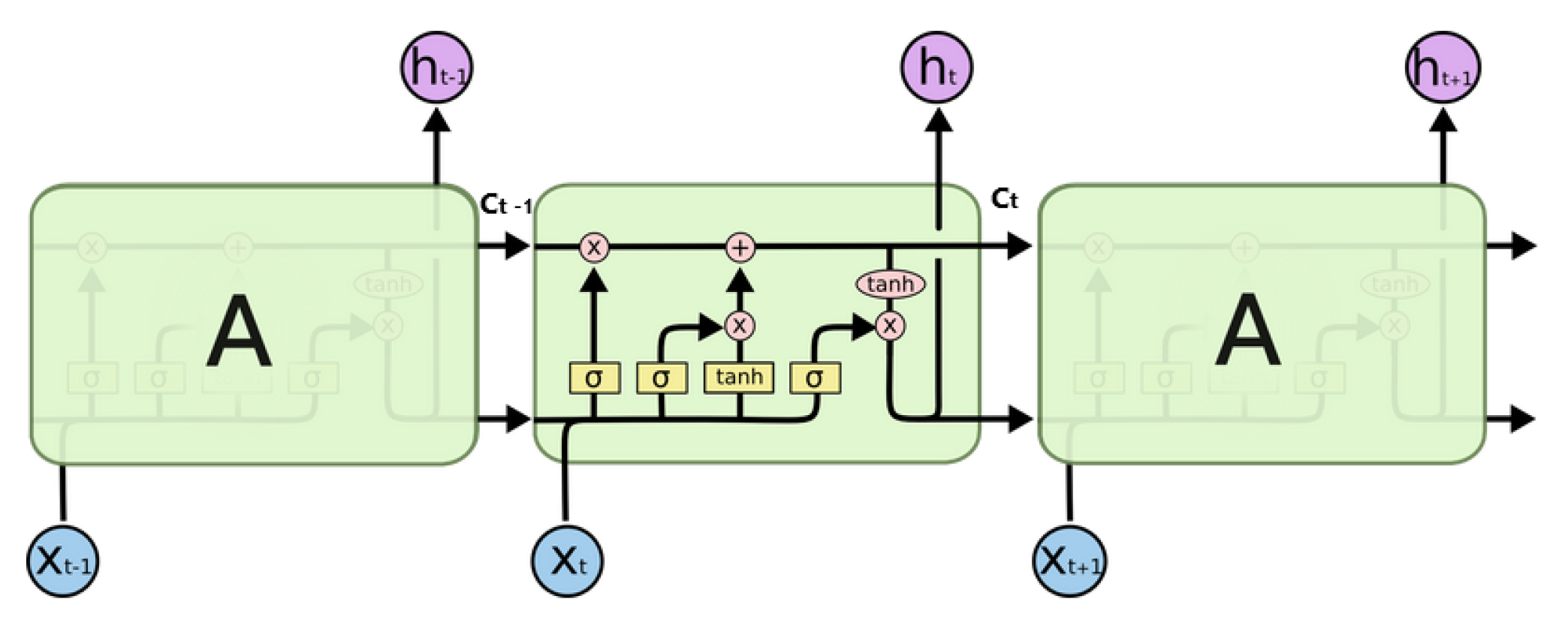
Sequential data such as sensor measurements are a typical format of data in prognostics problems [2]. Recurrent neural network (RNN)’s are designed to work with these kinds of data formats and is therefore considered to be suitable for prognostics. Among RNNs; long short-term memory (LSTM) and gated recurrent unit (GRU) are the most used. In general, the vanilla LSTM is indicated to give the best results.

One of the most popular datasets used for research related to RUL predictions is called C-MAPSS [3]. It is a collection of four datasets obtained from simulated degradation on turbofan engines. They consist of nominal and fault of turbofan engines and their degradation over several flights. In 2008, a competition to predict the most accurate RUL on a related turbofan engine dataset was arranged by the IEEE Prognostics and Health Management Conference. These datasets are often used in prognostics research.

Heimes et al. [4] proposed a method for predicting RUL using traditional RNN trained with back-propagation and extended Kalman Filter training. Their results were accurately able to predict the RUL and therefore received second place in the 2008 PHM competition. Instead of using a pure linear RUL label, they used a piece-wise linear RUL label, which has become accepted as the best labelling approach so far. In this approach, the label is constant until a certain level of degradation is reached; from then, it is linearly decreasing. The degradation point is selected to be the same for all sequences. In 2019, Ellefsen et al. [5] proposed an alternative labelling approach which resulted in one of the best performances on the C-MAPSS dataset so far. The approach is an adaptive version of the piece-wise linear RUL labels. In this approach, the starting point of the linear RUL decrements based on faults in the system selected individually for each sequence.

Others have also used the C-MAPSS dataset for their research. Wu et al. [6] used LSTM to estimate RUL. In addition, they compared the performance with traditional RNN and GRU. They found that the LSTM performed much better. In 2016, Yuan et al. [7] also used LSTM on turbofan engines, but for both diagnostics and prognostics. They aimed to predict a piece-wise linear RUL label and the probability of fault occurrences. The dataset did not contain fault labels, so they used an support vector machine (SVM) approach to detect anomalies and use them for labelling faults. Similar to other research, they compared their RUL predictions with other variants of RNN, but found the standard LSTM to perform better. Ellefsen et al. [8] proposed a deep semi-supervised architecture for predicting RUL on turbofan engines (C-MAPSS). The approach used a layer of restricted Boltzmann machine (RBM) for weight initialization and feature extraction, together with LSTM and finally a feed-forward neural network (FNN) layer for the final prediction. The proposed architecture achieved good results compared to pure supervised approaches. In 2017, Zheng et al. [9] combined sequences of LSTM-layers and normal FNN-layers to estimate RUL on both turbofan engines and milling machines. They state that their approach performs better than traditional methods. Their approach used a piece-wise linear RUL label. According to them, this labelling approach is not general enough and should be explored further.

Malhotra et al. [10] highlighted the problems with assumptions on degradation following a linear or exponential curve. They proposed a method that combined LSTM and encoder-decoder architecture for obtaining an unsupervised health index. The health index is then used to train a regression model that predicts RUL. The approach proves to be promising and achieves better results than several others that make normal degradation assumptions on the same datasets. Hinchi and Tkiouat [11] proposed an approach that combined LSTM and convolutional neural network (CNN). A convolution layer was used to extract features directly on vibration data from rolling bearings. The features were passed to an LSTM-layer that predicted the RUL on the bearings. The results are promising, but the authors state that further work needs to be done to include uncertainty in the predictions. In 2018, Zhang et al. [12] proposed a method based on LSTM to predict a capacity-oriented RUL on lithium-ion batteries. In order to introduce uncertainties to the predictions, they used a Monte Carlo simulation method.

Having a few samples of failure progression is a typical problem in prognostics research that Zhang et al. [13] highlighted. They used a Bi-directional LSTM for RUL prediction but experimented with transfer learning by pre-training the network with a different, but related dataset. Finally, the model is fine-tuned with the exact dataset. The results show that the transfer learning approach in general improved the prediction accuracy on datasets with few samples. The use of transfer learning in prognostics is investigated further in this work.

Yoon et al. [14] proposed an approach based on combining variational autoencoder (VAE) and RNN to predict RUL on turbo engines. Their approach used the encoder part of a VAE to reduce the dimensions of the data. Tang et al. [15] used a combination of sparse autencoder (SAE) (for feature extraction) and LSTM to predict bearing degradation performance. The results show better performance than traditional methods such as principle component analysis (PCA)-LSTM, SVM, and FNN. Senanayaka et al. [16] used a similar approach. They used a combination of autoencoder (AE) for unsupervised feature extraction and LSTM for prognostics on bearings.

CNN has also been used for predicting RUL. Babu at al. [17] used a deep CNN for estimating RUL on turbofan engines. The network consisted of two stages of convolution and pooling for automatic feature learning before a fully connected FNN was used to do the final RUL prediction. The input data consisted of sensor values structured into a 2D-format where each column represented a time-step, while each row was a specific type of sensor measurement. In 2018, Li et al. [18] used a similar approach based on a sliding window to structure the data in a 2D-format. They optimized their solution in terms of the number of convolutional layers and the size of the time window to achieve accurate results.

Deutsch and He [19] proposed a method based on deep belief network (DBN) in combination with a FNN for predicting RUL on rotating components. The method tries to use the strengths of DBN for feature extraction and FNN for its prediction power. The approach was compared with a model where feature extraction was done with a particle filter-based approach instead of DBN. They achieved quite similar results. Simpler DL techniques such as a FNN with several hidden layers have also been used towards PHM. Tian [20] used age and sensor measurement from present and previous inspections as input to an FNN with two hidden layers. The method was applied to predict RUL in the form of a percentage of health state on bearings.

Among the attempted approaches on prognostics, LSTM and CNN seems the most promising. Both methods and FNN is used for prognostics in this paper. Both the piece-wise linear RUL labelling approach and the newly proposed adaptive approach are used for labelling. The next section presents how maintenance on air compressors is done today.

3. Theory

This section briefly introduces theory on the DL methods used in this project. A more detailed description of the theory can be found in the master thesis [21] that this work originates from.

3.1. Feed-Forward Neural Network

Feed-forward neural network (FNN) is a type of cyclic ANN. It is considered to be the first and simplest type of ANN. An FNN consist of multiple, simple, processing units called neurons, organized into layers [22]. A neuron can have multiple inputs but only one output, which can be distributed to other neurons. Neurons are interconnected with weighted connections that are used to transfer signals. Neurons in the input layer get activated from input data, while neurons in other layers are activated through weighted connections [22]. The output of a neuron is either an input to another neuron or an output of the model. A neuron’s output is determined from the sum of the weighted inputs passed through an activation function.

3.2. Long Short-Term Memory

LSTM is a variant of RNN designed to learn long-term dependencies [23]. The LSTM introduces the idea of a memory cell, which contains gates that tries to regulate the information through the cell. The result is a network that achieves contextual weights that can deal with long-term dependencies flexibly. Several variants of the LSTM have been introduced, such as the Vanilla LSTM [24] and GRU-LSTM [25]. The Vanilla LSTM has proved itself popular for PHM; therefore, it is the preferred variant of LSTM in this project. Many variants of the Vanilla LSTM exist [26]. In this work, the Vanilla LSTM without peephole connections were used. The Vanilla LSTM (referred to as just LSTM from now on) has four interacting NN layers. The architecture of an LSTM and its memory cell is illustrated in Figure 1.

3.3. Convolutional Neural Network

CNNs are a type of DL techniques known for their performance on images. They have been used to classify images, cluster images, identify faces, and much more [28]. Although they are often mentioned for images, they can also be used for 1D-data, e.g., time-series or 3D-data such as videos. A CNN is an artificial neural networks (ANN) model that uses convolution operations in at least one layer. CNN has become popular due to its ability to extract important features from input data automatically. One of the motivations for using CNN is that it reduces computation requirements due to weight sharing [29]. A typical CNN consist of four types of layers: convolutional, pooling, flattening and fully connected [30].

3.4. Particle Swarm Optimization

Particle swarm optimization (PSO) is a robust stochastic optimization technique based on swarm behavior [31]. It was originally introduced to optimize continuous, non-linear functions, but other versions of the algorithm can also solve binary and permutation problems. In the topic of machine learning (ML), PSO has among other things been used as a training algorithm for the weights in a neural network (NN) [32] and for optimization of ML hyper-parameters [33,34]. In this project, PSO is used for tuning hyper-parameters.

The PSO is based on a swarm of particles that aims to find x that minimizes an objective function $f\left(x\right)$ [35]. First, the swarm of particles with size N is initialized where each particle is assigned a random position, X, in the search space with the velocity V. Internal parameter settings such as the maximum number of iterations and weights are also assigned. At every iteration, the position of each particle is evaluated based on the objective function. Each particle keeps track of their personal best solution throughout a search. The algorithm keeps track of the global best solution among all particles as well. The next step of the PSO is to update the velocity and position of each particle. The velocity is determined based on the three factors: inertia, personal influence, and influence by the society. Inertia is considered a way to keep the momentum and is found with Equation (1), where w is the inertia weight, and $v_i\left(t\right)$ is the previous velocity.

$$\mathit{Inertia}=w\ast v_i\left(t\right)$$

(1)

The personal influence lets a particle i to move towards its personal best solution so far. It is determined by Equation (2), where $c_1$ is an acceleration coefficient, $r_1$ is a random number between 0 and 1, $p_i$ is the personal best solution and $x\left(t\right)$ is the current position.

$$\mathit{Personal} \mathit{Influence}=c_1\ast r_1(p_i-x_i\left(t\right))$$

(2)

The influence by the society lets a particle move in the direction of the global best solution. It is found from Equation (3), where $c_2$ is an acceleration coefficient, $r_2$ is a random number between 0 and 1, $p_g$ is the global best solution and $x\left(t\right)$ is the current position.

$$\mathit{Global} \mathit{Influence}=c_2\ast r_2(p_g-x_i\left(t\right))$$

(3)

These three factors update the velocity of a particle with Equation (4), where w, $c_1$ and $c_2$ are parameters used to adjust the behaviour of the algorithm. A large w (inertia weight) gives the algorithm better exploring abilities, while smaller values mean better exploiting capabilities. Exploitation can also be achieved by having larger $c_1$ than $c_2$. The opposite gives better exploration ability.

$$v_i(t+1)=w\ast v_i\left(t\right)+c_1\ast r_1(p_i-x_i\left(t\right))+c_2\ast r_2(p_g-x_i\left(t\right))$$

(4)

Finally, the position x of each particle is updated with Equation (5).

$$x_i(t+1)=x_i\left(t\right)+v_i(t+1)$$

(5)

After updating the position of all particles, the search loop either continues or stops if the search criterion’s is met. Such search criteria can be maximum number of iterations or no improvements for k iterations [35].

4. Methodology

Prognostics is often concerned with predicting the RUL of a system. In this project, it is explored towards predicting the RUL of air compressors with DL techniques. These experiments’ goal is to find a technique able to predict the RUL accurately and help prevent unexpected standstills and better plan when to do maintenance. Predicting RUL is not something new, but according to the researched literature, it has not been done on air compressors.

This research on prognostics includes two main sub-parts. An overview of these topics is listed below.

• Explore three different DL techniques for predicting RUL to find the most promising method.
• Explore if transfer learning is promising in prognostics. Investigate if a different prognostics dataset can improve the predictions.

Predictions must be early enough to start maintenance activities before it is too late. Predictions should not over-estimate the RUL. Under-estimating is not as bad, but it means that maintenance actions might be taken before it is necessary. The predictions are explored with three different types of DL models:

• FNN: Deep FNN is tested as the only model not taking sequences into account.
• LSTM: The related work indicated the LSTM as one of the best choices for predicting RUL.
• CNN: The CNN is used with the time-window approach described in the related works. It has also proven promising towards prognostics.

4.1. Data

22 datasets from an air compressor were collected to conduct the relevant experiments. The air compressor is equipped with 14 sensors measuring temperatures, pressures, and current from different system parts. The compressor datasets were collected in a controlled environment, where the faults are forced. Three different types of datasets were collected; normal data and two different types of faults. The sequences with faults start in normal operating conditions, but a fault is gradually introduced to the system, leading to degradation of the air compressor. The end of the sequences is considered the end-of-life of the compressor. That is also the point that is tried to predict the time until.

The two types of faults are just referred to as faults A and B. This is due to a confidentiality agreement with the company producing the compressors. This also means that the specific sensors’ measurements, time scale, and fault/failure source cannot be disclosed.

Table 1. Data usage for training and tuning.

Prognostics: Data Usage for Tuning
Type	# Datasets	Training	Validation	Testing
Normal	8	8	0	0
Fault A	7	5	1	1
Fault B	7	5	1	1

shows which datasets are used for training, validation, and testing during the models’ tuning process.

Table 2. Data usage for evaluating the model prognostics predictions.

Prognostics: Data Usage for Evaluation
Type	# Datasets	Training	Testing
Normal	8	8	0
Fault A	7	6 *	1 *
Fault B	7	6 *	1 *

* Iterative process with k-fold cross validation.

shows the usage when evaluating the model performance.

In k-fold cross-validation, the data is randomly split into k distinct folds. The model is then trained and tested k times, picking a different fold for evaluation every time and training on the other k-1 folds. The result is an array containing the k evaluation scores. An average score can be used as an estimate of the performance of the model. K-fold cross-validation comes at the cost of training your model k times; however, it gives more accurate estimates of the model’s overall performance and enables the use of the whole data available for training your model without sacrificing a holdout test set. These models were evaluated with k-fold cross-validation, where the results are the mean of the results for each fold. 7 folds were used, meaning that each dataset was used once for testing. K-fold cross-validation is also a preventative measure against the typical problem of overfitting when working with small datasets.

A common problem when working with ML, especially for prognostics, is having a few training examples. Data augmentation is a term used for increasing the data foundation by augmenting existing examples. For images, this can typically be to rotate, skew, flip, and add noise. In this work, the data is multivariate time-series data, consisting of few run-to-failure examples. Data augmentation was used to create more run-to-failure examples from the initial sequences. If the data is sampled 10 times each second, one run-to-failure example can be split into 10 new run-to-failure examples. This can be done by using the 10 first samples as the first sample in 10 new sequences. Next, every 10 sample is used in each of the new sequences. The first run-to-failure example will then contain sample numbers 1, 11, 21, 31, and so on. This approach gives more samples for every value of the RUL label, but there is a significant restriction to note. The new sequences that originate from the same sequence will, in theory, have values drawn from the same statistical distribution. Therefore, all sequences originating from the same original sequence are used for the same purpose (e.g., training) to avoid information leakage. This also yields for the k-fold cross-validation. In the experiments, data augmentation is used to generate 5 new sequences from each original sequence.

4.2. PHM08 Challenge Data

The 2008 PHM conference competition used a dataset that has several run-to-failure examples for turbofan engines [36]. The competition’s goal was to explore techniques for prognostics and get the most accurate RUL predictions. The dataset is based on an aero-propulsion system simulator called C-MAPSS. The simulator simulates degradation in turbofan engines and collects many sequences where the condition goes from the normal condition until failure. Each sequence has different running conditions, initial wear, and noise levels. The data contains 21 sensor measurements and 3 signals referred to as operational settings. The PHM08 challenge dataset is a part of a larger and more complex dataset referred to as the C-MAPSS dataset in the literature. These datasets are the most used within the field of PHM and especially when it comes to RUL predictions. In this paper, the PHM08 dataset was used for experimentation of transfer learning in the field of prognostics.

4.3. Labelling

RUL is the number of time units (seconds, hours, cycles, etc.) until a system fails or breaks. The last sample in a sequence is considered to be end-of-life. The goal is to predict the time until end-of-life. The available literature has indicated that the piece-wise linear RUL labelling approach is accepted as the best. It emphasizes the fact that systems do not show signs of degradation until a certain level is reached or a fault has occurred. The RUL is decreasing linearly from that point on. Therefore the RUL is kept constant until the last X samples. The constant level must be chosen based on how long in advance predictions should or could be taken.

Figure 2 shows an example of the normal piece-wise linear RUL label, where the constant level was chosen to be 100. It shows three sequences of different lengths (200, 225, and 250).

4.4. Scoring

For this project, mean absolute error (MAE) (Equation (6)) and root mean squared error (RMSE) (Equation (7)) were selected to evaluate the performance. MAE gives a descriptive output which says how much the predictions differs from the target in general. Another function was selected as loss-function. It penalizes over-estimates more than under-estimates was. This is selected due to a more severe consequence when over-estimating the RUL. The asymmetric absolute error [37] is chosen. The function is quite similar to the ordinary MAE-function. The difference is that when the prediction over-estimates, the absolute value of the error is multiplied with $\beta$. If it under-estimates, the absolute value of the error is multiplied with $\alpha$. If $\beta >\alpha$ over-estimates are penalized more than under-estimates. In present work, $\alpha =1.8$ and $\beta =2.2$.

$$\mathit{MAE}=\frac{1}{N}\sum _{i=1}^N\left|\right|t_i-y_i\left|\right|$$

(6)

where $\mathit{MAE}$ is the loss, N is the number of outputs, $t_i$ is the desired output and $y_i$ is the actual output.

$$\mathit{RMSE}=\sqrt{\frac{1}{N}\sum _{i=1}^N{(t_i-y_i)}^2}$$

(7)

where $\mathit{RMSE}$ is the loss, N is the number of outputs, $t_i$ is the desired output and $y_i$ is the actual output.

The choice of scoring and loss-function is selected manually based on experience. In the future, a more thorough exploration of loss and scoring for prognostics should be done.

4.5. Transfer Learning

Transfer learning was investigated towards trying to improve the predictions and potentially reduce the need for run-to-failure examples. Transfer learning is much used in object detection in images, where re-using parts of an already-trained network can improve predictions and reduce the number of needed training examples.

Transfer learning can be performed in several ways. Commonly, transfer learning refers to when a model is trained to solve a problem, then reused to solve another (potentially related) problem. The model could be reused directly but retrained on data from the new problem. Another approach is to take layers from the original model and reuse them for the new problem in a new model. These layers are then transferred by initializing layers of the same size and weights as the transferred layers in the new model. These layers can be used in two ways:

• Trainable layers: The weights are then only used as an initialization with the idea that the weights are closer to the optimal value than if they are initialized randomly.
• Untrainable layers: In these cases, the layers’ weights are frozen, meaning that they cannot be updated during training. The idea here is that the original model already learned optimal features.

The concept of transfer learning in the field of prognostics has so far received little attention. A part of this case was to investigate the effects of using transfer learning for this purpose. The PHM08 dataset was used to build a good performing model. The model was then used to transfer learning to new models to perform on the compressor dataset. 8 different model architectures were tested to predict RUL on the compressor dataset. The models are involved in a transfer learning process to improve air compressors’ predictions by transferring both trainable and untrainable layers.

5. Model Configuration

The hyper-parameters and architectures for each model were tuned using PSO. The selected PSO-specific parameters are displayed in

Table 3. PSO-specific parameters.

Parameter	Values
Inertia	0.5
Cognitive	0.8
Social	0.6
#Particles	10
#Iterations	10

. Every model was first tuned manually to find promising regions of architecture before running the optimization loops.

5.1. FNN

Among the four optimizers (SGD, RMSProp, Adam, and AdaGrad), Adam was selected to give good results in manual experiments. The experiments indicated that a FNN with three hidden layers were most promising. Dropout was used between the hidden layers.

Table 4. FNN hyper-parameters for prognostics.

Hyper-Parameter	Values
Learning rate	0.001, 0.0001, 0.00001
Batch size	10, 25, 50
Units layer h1	10, 20, 30, 40
Units layer h2	10, 20, 30, 40
Units layer h3	10, 20, 30, 40
Dropout	0.0–0.3 (0.2)
Activation	sigmoid, tanh, ReLU

shows the parameters that were tuned with PSO and the best parameters found are highlighted.

5.2. LSTM

Through manual experiments, many architectures for the LSTM was tested. The most promising architecture was with three LSTM layers and two dense (FNN) layers. The last dense layer is the output layer. The RMSProp optimizer was selected based on its performance in manual experiments. The output activation function is mentioned as tanh. For the LSTM layers, the tanh activation function was used (default), but the activation function for the dense layers was tuned with PSO. The training was performed with 30 epochs and early stopping.

Table 5. LSTM hyper-parameters for prognostics.

Hyper-Parameter	Values
Learning rate	0.001, 0.0005, 0.0001, 0.00005, 0.00001
Batch size	10, 40, 70, 100
Units layer LSTM1	10, 15, 20, 25, 30, 35, 40
Units layer LSTM2	10, 15, 20, 25, 30, 35, 40
Units layer LSTM3	10, 15, 20, 25, 30, 35, 40
Units layer Dense1	5, 10, 15, 20, 25, 30
Activation	Sigmoid, tanh, ReLU
Time window	5, 10, 15, 20, 30, 40, 50

shows the parameters that were optimized with PSO, the best parameters found are highlighted in the table.

5.3. CNN

CNN is a model with many parameters to tune. Manual experiments were performed to find the most promising architecture. These experiments indicated that the most promising architecture was to use two sets of convolutional layers and max-pooling layers. Next, flattening and then three dense layers. The final dense layer is the output layer. A padding strategy called same was used for all convolutional and max-pooling layer, except the final max-pooling layer where valid was used. This means that the dimension is reduced instead of keeping it. Dropout was added between the first two dense layers. The RMSProp optimizer was selected since it showed the most promising results. The remaining parameters were tuned with PSO.

Table 6. CNN hyper-parameters for prognostics.

Hyper-Parameter	Values
Learning rate	0.001, 0.0005, 0.0001, 0.00005, 0.00001
Batch size	10, 40, 70, 100, 130
#Filters-Conv2D (1)	4, 8, 12, 16, 20
Kernel size-Conv2D (1)	4–10 (5)
Kernel size-Pool (1)	2, 3, 4
#Filters-Conv2D (2)	4, 8, 12, 16, 20
Kernel-Conv2D (2)	5–10 (4)
Kernel-Pool (2)	2, 3, 4
Units -Dense (1)	10, 20, 30
Units -Dense (2)	4, 8, 12, 16, 20
Dropout	0.0–0.3 (0.15)
Activation	sigmoid, tanh, ReLU
Time window	5, 10, 15, 20, 30, 40, 50

shows the tuned parameters, and the best parameters are highlighted.

6. Results

6.1. Compare Models

After the best architecture and hyper-parameters were found, each model was trained and evaluated using k-fold cross-validation. The models’ performance was mainly evaluated with MAE, which indicates the average error from the target. RMSE was also used, which punishes large errors more.

Table 7. Results from RUL prediction using k-fold cross validation.

	RMSE	MAE
FNN	14.04	9.27
LSTM	11.03	6.87
CNN	13.14	8.34

shows the MAE and RMSE for each of the models on the averaged performance from k-fold cross-validation.

The results show that there were some large differences between the models. The LSTM was clearly performing the best with a MAE of 6.87. This means that the model on average predicted 6.87 time units from the target. The second best model was the CNN, and worst was FNN.

Table 8. Results from RUL predictions on each individual split.

	MAE
Models	Split 1	Split 2	Split 3	Split 4	Split 5	Split 6	Split 7
FNN	4.00	7.16	33.10	2.42	6.93	4.45	6.85
LSTM	4.92	6.04	22.04	3.77	3.72	1.85	5.76
CNN	3.70	6.10	26.91	5.07	5.00	3.81	7.81

shows the MAE on each individual split. The table indicates that the performance on split 3 was much worse than for the other splits. The LSTM achieved an average MAE of 22, and as high as 33 for FNN. Since the results shows that split 3 performs the worst, it can be assumed that the data was collected under quite different conditions or operation. We have discussed it further later.

When excluding split number 3 the predictions from the LSTM model were on average 4.34 time units away from the correct RUL. So far, the RUL predictions have only been evaluated based on the performance measure. The predictions were also analyzed visually. This makes it possible to notice if the predictions were fluctuating, over-estimating, under-estimating, etc. Next, predictions from each model is analyzed visually.

6.2. FNN

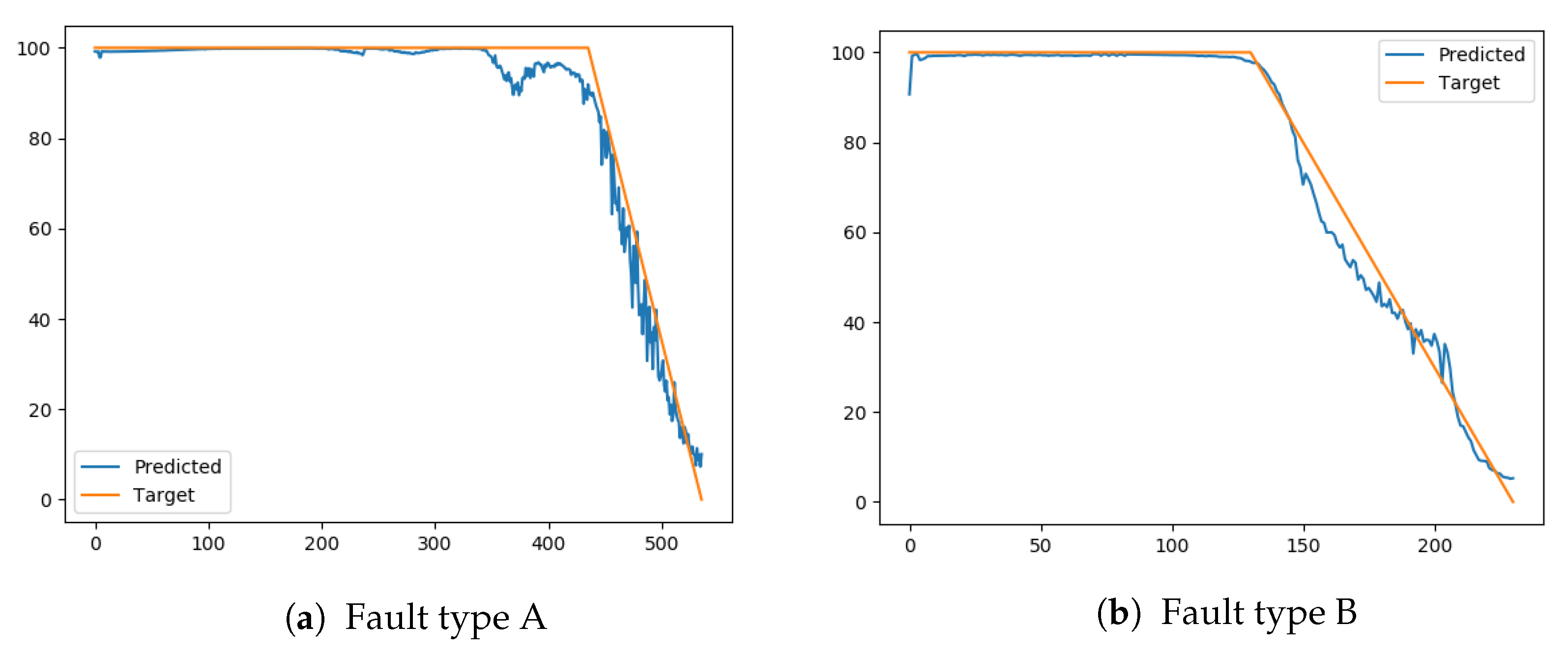
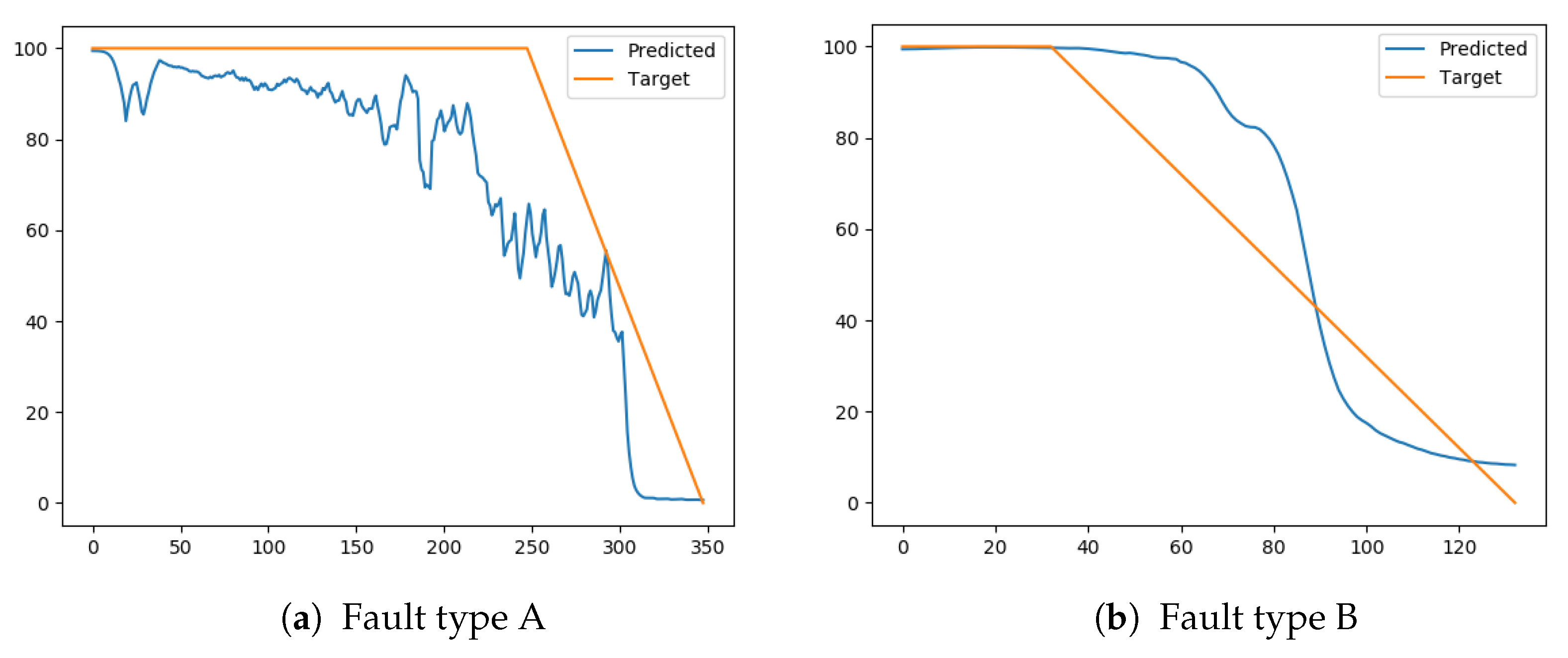
First, the FNN predictions were explored. Split number 4 achieved a MAE of 2.42. Figure 3a,b shows the predictions on one sequence of each fault type from that split. The figures prove that the predictions were accurate and very close to the actual RUL of the compressor.

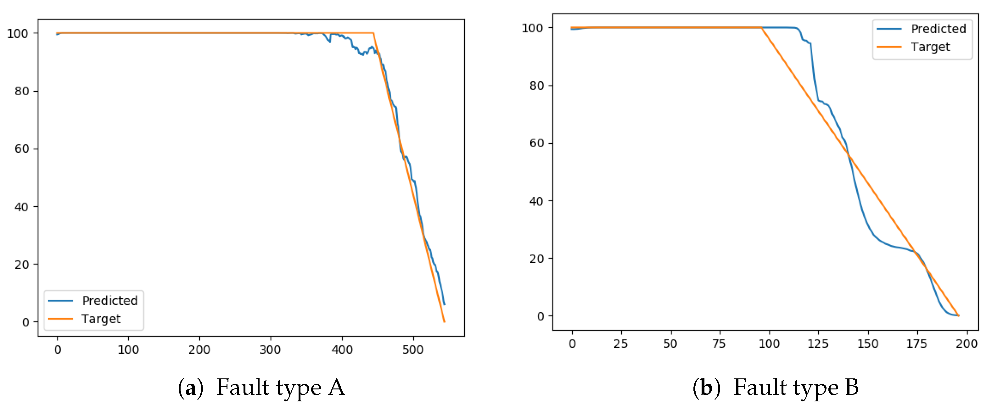
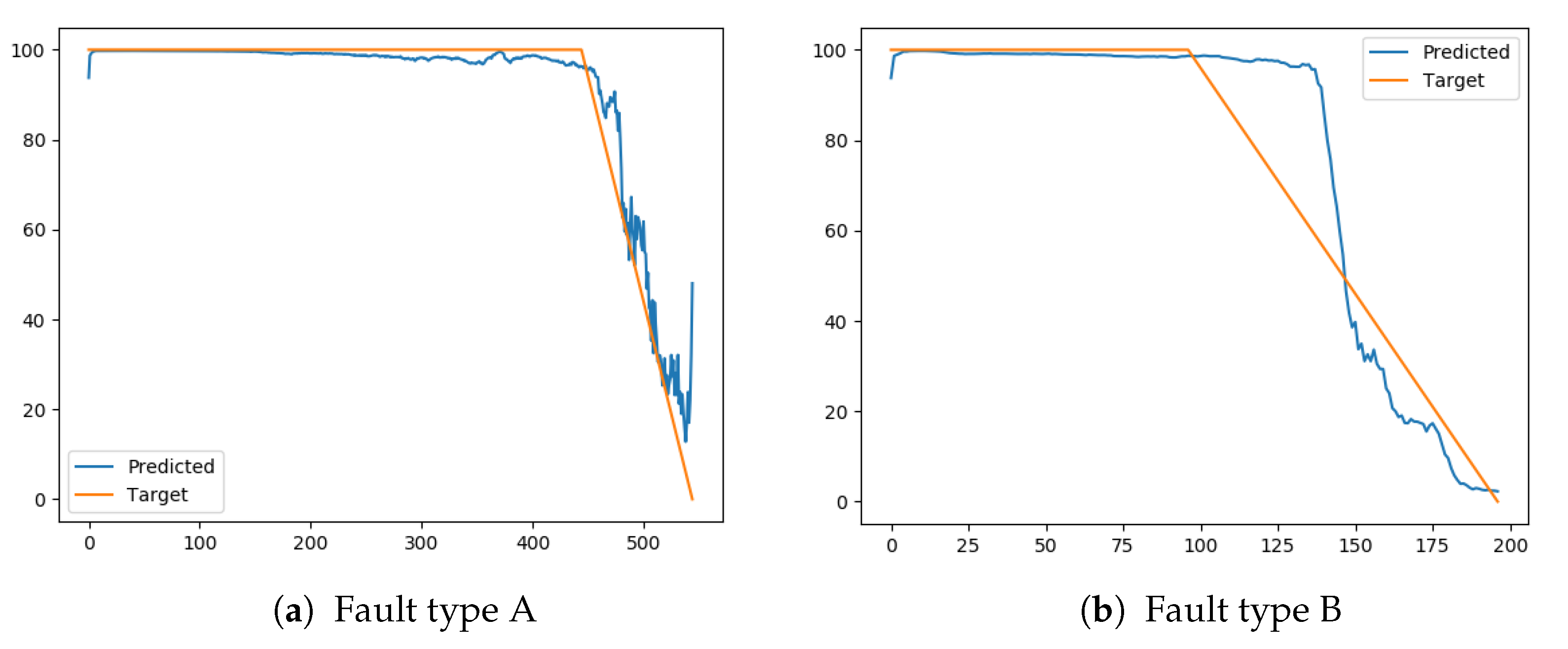
The FNN achieved variable results for the other splits. On split number 6, it achieved a relatively low MAE, but as Figure 4a indicates, the predictions on a sequence with fault type A from split 6 had much noise. Several of the predictions from FNN on sequences with fault type A have similar fluctuations. This could have been reduced by applying a moving average filter. Figure 4b shows that the predictions on a sequence with fault type B followed the target relatively good. It had less noisy, but were a bit late to start predicting the linear RUL.

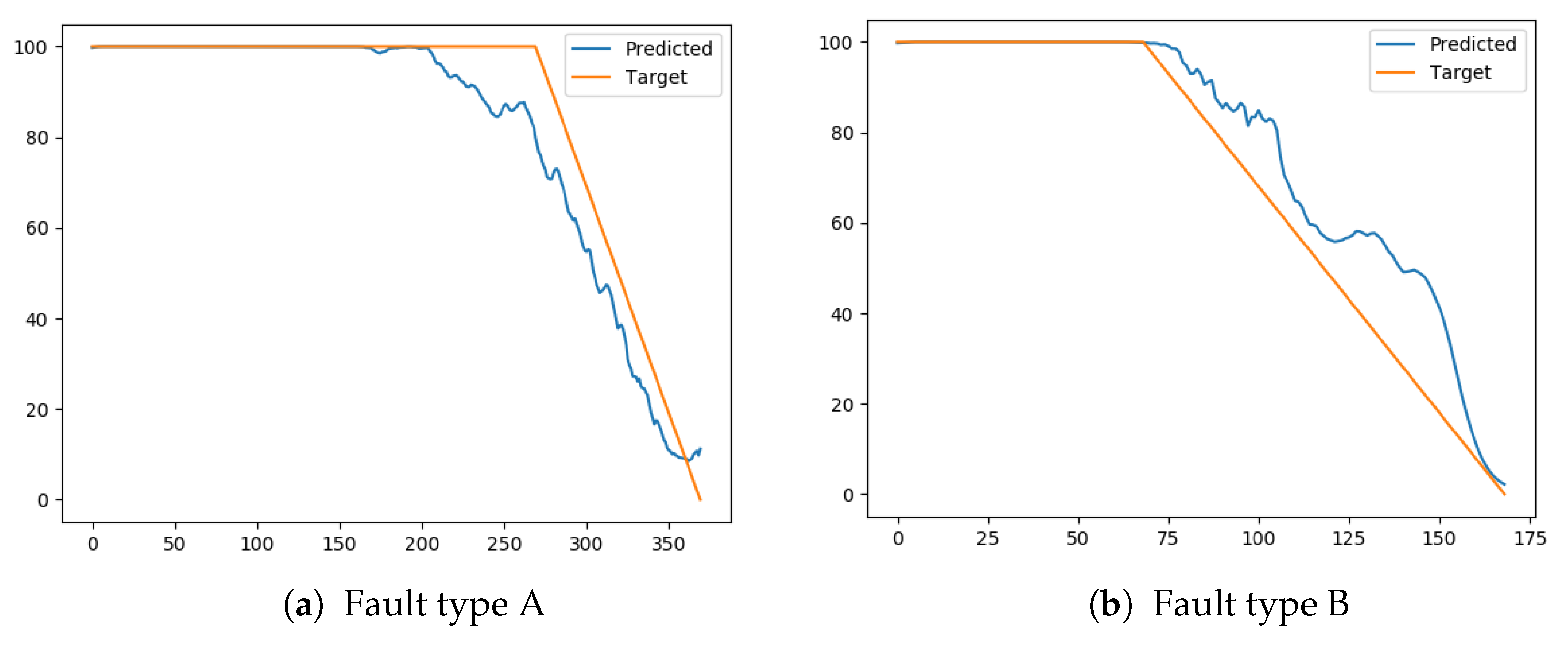
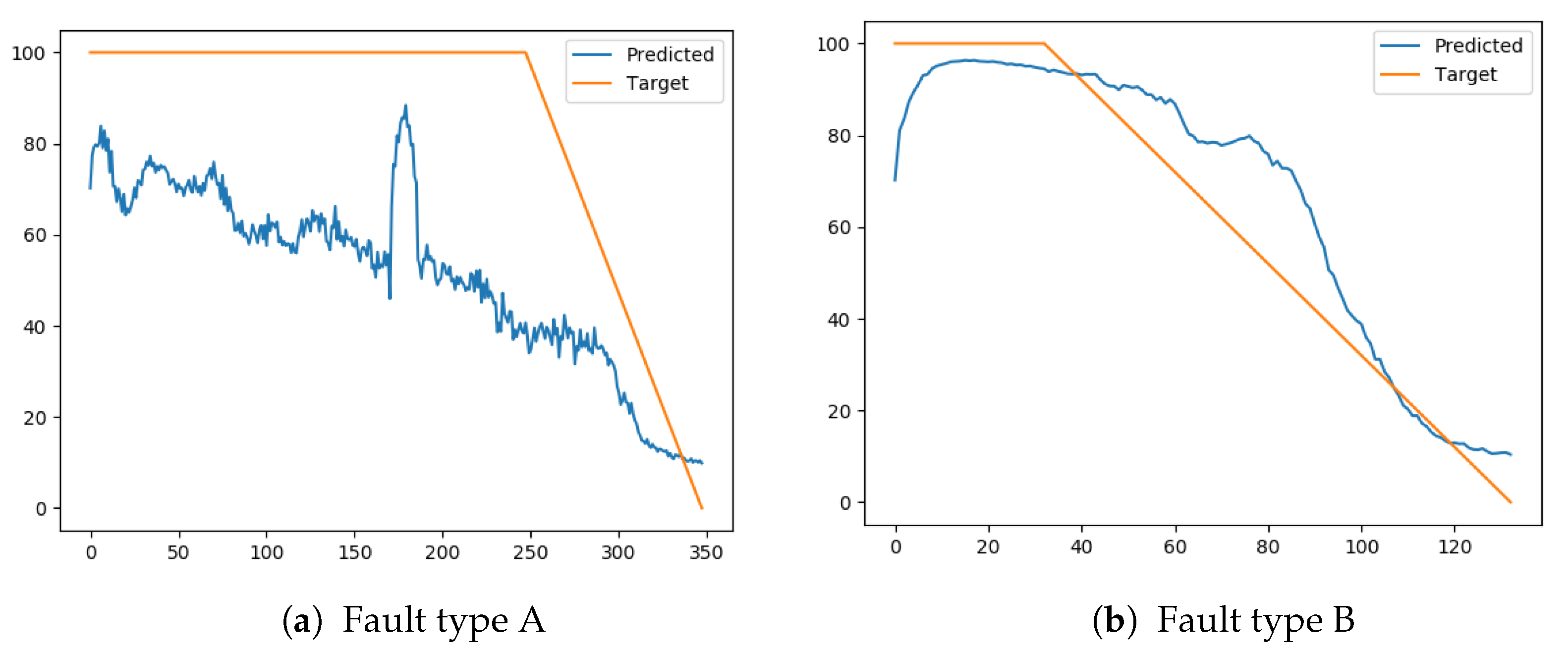
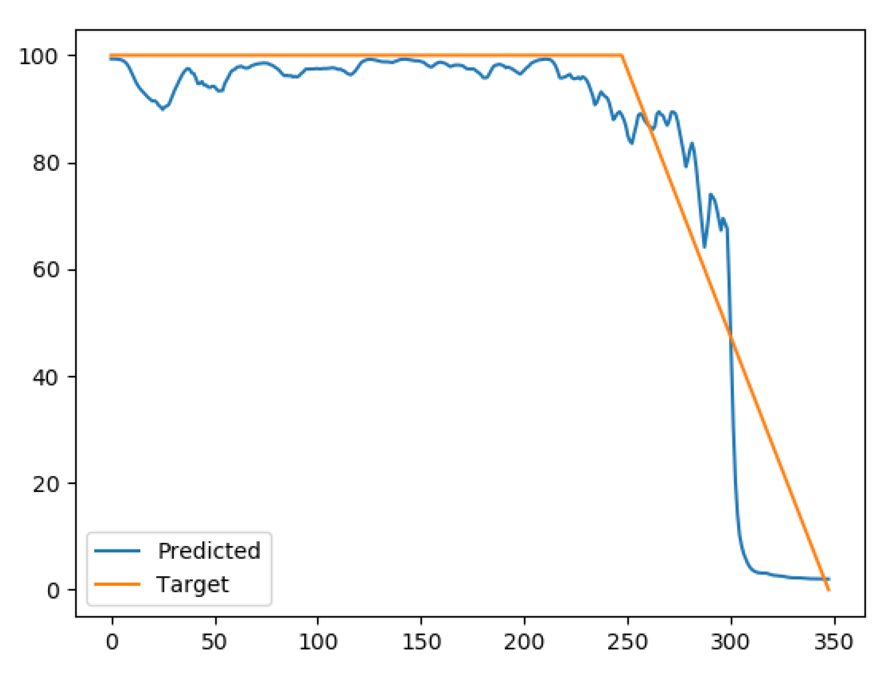
As indicated earlier, predictions on split number 3 have performed much worse than the others. This is proven in Figure 5a,b, which are predictions on a sequence with fault A and B from split 3. The predictions on the sequence with fault type A were far from the target and under-estimated the RUL by a lot. The other sequence was over-estimated large parts of the linear RUL.

6.3. LSTM

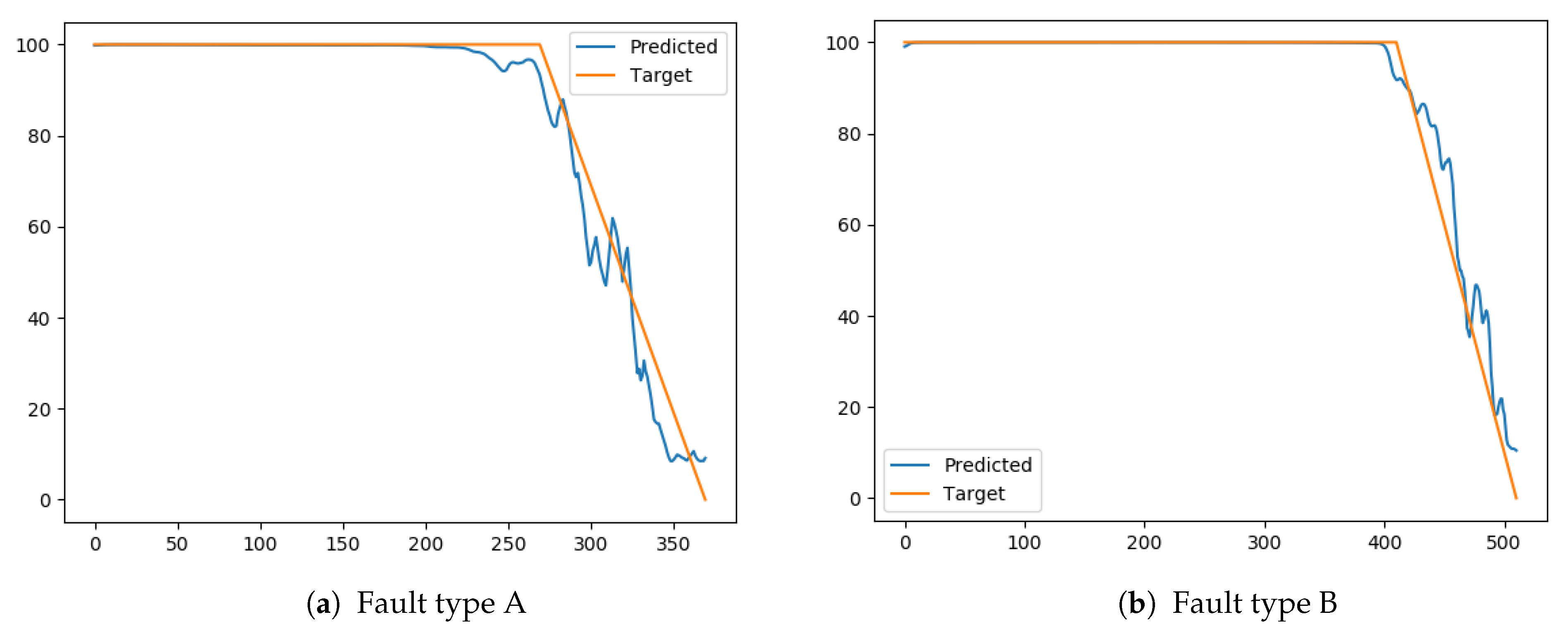
Predictions from the LSTM model achieved the lowest MAE and can be considered the best performing model. Figure 6a shows that the model was accurately predicting the RUL on a sequence with fault type A from split 6. The predictions from the same split, but on a sequence with fault B is not as accurate, but still a good prediction.

Predictions on split number 7 achieved a higher MAE than four other splits. The sequence with fault A slightly under-estimated the RUL (Figure 7a), while the sequence with fault B is over-estimated a little. Under-estimation is considered better since the maintenance can be done before something breaks. Over-estimation may lead to failure before maintenance actions took place.

As stated earlier, both the LSTM and FNN achieved the highest MAE on split number 3. Figure 8a shows that the LSTM predictions on the sequence with fault A were not as accurate as the ones seen so far. It was more accurate than FNN on the same sequence. The predictions under-estimated the RUL, but were at least able to indicate that the system was degrading in advance of a failure. The sequence with fault B over-estimated less than the FNN prediction, and even under-estimated the target towards the end-of-life. This is indicated in Figure 8b.

The LSTM has proven superior to the FNN both when it comes to the score and the visual analysis. The LSTM achieved satisfactory results for all splits, except split 3. The results on split 3 were at least better for LSTM than for FNN.

6.4. CNN

The MAE showed that the CNN performance was ranked between FNN and LSTM. The best CNN results were achieved on split 1. The prediction on a sequence with fault A and B from that split is shown in Figure 9a,b, respectively. The results for fault A show that the prediction slightly over-estimated the RUL in early stages of degradation. The other sequence shows that the RUL was estimated accurately until about 30 time units were remaining.

The CNN achieved varying results on split 6. The predictions on a sequence with fault A (Figure 10a) were following the target closely, but with some noise, especially towards the end-of-life. The model performed worse on the sequence with fault B, where the reduction in RUL was detected too late. It over-estimated the early linear phase of the prediction.

Figure 11a shows that the CNN also struggled with predicting the RUL on the sequence with fault A on split 3. The prediction under-estimated the target by a lot for almost the entire sequence. The results on the sequence with fault B were not as bad, but it over-estimated the RUL mid-sequence (Figure 11b).

6.5. Summary

The results have indicated that there were considerable differences in the three DL models’ performance. LSTM performed best and therefore considered the best model for predicting RUL, in this particular case. The predictions were accurate, and they were on average missing in the upper edge of 6 time units from the target. This is promising results. Next, it is explored how transfer learning can be used in prognostics, and if it can improve the results.

6.6. Transfer Learning

Transfer learning was researched to see if the results could be improved using datasets on other equipment degradation. If so, it contributes to reducing the required number of run-to-failure examples. It was investigated with LSTM, which has performed the best in the previous prognostics experiment. Transfer learning was used by first training a model to perform well on the much larger and popular dataset within prognostics research, called PHM08 (see Section 4.2). The model was built to match the LSTM architecture that performed well on the air compressor’s prognostics experiments, making it easier to use transfer learning.

The architecture and parameters of the LSTM model on the PHM08 dataset were decided based on experience and manual experiments. The best results were achieved using a model consisting of four LSTM-layers and two dense layers. The number of neurons in each layer is described in

Table 9. Architecture for the transferred model.

Layer	Units
LSTM layer 1	20
LSTM layer 2	30
LSTM layer 3	30
LSTM layer 4	30
Dense layer 1	20
Dense layer 2	1

. The same setup as for the experiments with the air compressor data was used to train the model. This means that the labels were normalized between −1 and 1, the time window was 20, and activation functions for all layers were tanh. Since the number of inputs was not equal, the first LSTM-layer of the PHM08-model was not reused.

Transfer learning typically means to take parts of another trained network and reuse it in a new network either with untrainable or trainable layers. Several different architectures were explored. The architectures were based on:

• Re-using parts of the model, but make the layers untrainable.
• Re-using parts of the model, but make the layers trainable.
• Combining both untrainable and trainable layers.

To explore if transfer learning can contribute to improve the RUL predictions on the air compressor, several architectures were tested. The layers from the trained PHM08-model were used either untrainable or trainable. In the described architectures, a layer from the PHM08-model is referred to with PHM- plus the type of layer and the corresponding layer number (from Table 9). An example is if the second LSTM layer is used, it is referred to as PHM-LSTM-1, while a new LSTM layer is simply referred to as LSTM.

Table 10. The first and second proposed model related to transfer learning.

Model 1	# Nodes	Trainable	Model 2	# Nodes	Trainable
LSTM	20	Yes	LSTM	20	Yes
PHM-LSTM-2	30	Yes	LSTM	30	Yes
PHM-LSTM-4	30	Yes	PHM-LSTM-4	30	Yes
PHM-Dense-1	20	Yes	PHM-Dense-1	20	Yes
PHM-Dense-2	1	Yes	Dense	1	Yes

,

Table 11. The third and fourth proposed model related to transfer learning.

Model 3	# Nodes	Trainable	Model 4	# Nodes	Trainable
LSTM	20	Yes	LSTM	20	Yes
PHM-LSTM-2	30	No	LSTM	30	Yes
PHM-LSTM-4	30	No	PHM-LSTM-4	30	No
Dense	20	Yes	Dense	20	Yes
Dense	1	Yes	Dense	1	Yes

,

Table 12. The fifth and sixth proposed model related to transfer learning.

Model 5	# Nodes	Trainable	Model 6	# Nodes	Trainable
LSTM	20	Yes	LSTM	20	Yes
PHM-LSTM-2	30	Yes	PHM-LSTM-2	30	No
PHM-LSTM-4	30	Yes	PHM-LSTM-3	30	No
PHM-Dense-1	20	Yes	PHM-LSTM-4	20	Yes
Dense	1	Yes	PHM-Dense-1	20	Yes
			Dense	1	Yes

and

Table 13. The seventh and eight proposed model related to transfer learning.

Model 7	# Nodes	Trainable	Model 8	# Nodes	Trainable
LSTM	20	Yes	LSTM	20	Yes
PHM-LSTM-2	30	No	PHM-LSTM-2	30	No
PHM-LSTM-3	30	No	PHM-LSTM-3	30	Yes
PHM-LSTM-4	30	No	PHM-LSTM-4	30	Yes
PHM-Dense-1	20	Yes	PHM-Dense-1	20	Yes
Dense	1	Yes	Dense	1	Yes

describes 8 different models that were tested to improve the predictions. Model 1, 2, and 5 uses several layers from the PHM08-model but allows the transferred layers to be trained. The pre-trained layers are, in such cases, used as a kind of weight initialization. The other models use a combination of new layers together with both trainable and untrainable layers. The reason some layers were untrainable is the idea that they might have been trained to find good and general features that the new model can benefit from.

All the stated models were trained with the RMSProp optimizer with a learning rate of 0.00005. A batch size of 40 was used, and the models were trained over 40 epochs. The time window was selected to be 20 time units. Results were evaluated based on MAE averaged over the 7 splits in k-fold cross-validation.

Table 14. Results from RUL predictions with transfer learning models.

Model	MAE
Original best	6.87
Model 1	9.81
Model 2	8.22
Model 3	9.58
Model 4	6.78
Model 5	8.41
Model 6	6.14
Model 7	7.45
Model 8	5.92

shows the score of each of the transfer learning models and the best model without transfer learning, referred to as original best. The models that performed better than the original best are highlighted in the table.

The results showed that three of the models performed better than the best model without transfer learning. Model 4 performed quite similar to it, while model 6 and 8 performed much better. These three models have in common that they have at least one untrainable layer from the PHM08-model. Model 6 and 8 also used several trainable layers from the PHM08-model. The difference between the two best models was that model 6 has two untrainable layers, while model 8 only has one. This indicated that having untrainable layers might force the network to reconstruct and benefit from good features in the transferred model.

The result from the best model (#8) for each individual split is presented in

Table 15. Results from RUL predictions on each split with model 8.

	MAE
	Split 1	Split 2	Split 3	Split 4	Split 5	Split 6	Split 7
Model 8	3.43	11.3	7.57	3.24	5.17	3.96	6.77

. Compared to the original model, the transfer learning model performed similarly for most of the splits, but there were large differences in split 2 and 3. The MAE was reduced a lot for split 3, while it increased a lot for split 2. It is hard to identify why this happens, but it might indicate that the original model was over-fitted to some degree, while the transfer learning model generalizes superiorly.

Figure 12a shows the prediction from model #8 on a sequence with fault type A from split 7. Figure 12b shows the prediction on a sequence with fault B from split 0. The predictions were following the target relatively good.

Split 3 resulted in quite bad predictions on the original model, but the best transfer learning model performed a lot better. Figure 13 shows the RUL prediction on the sequence with fault A from split 3. It shows that it was a lot better than the original predictions, but struggled to predict accurately close to end-of-life.

The results proved that using a model that was trained on sequences from a different system can contribute to improving predictions. Transfer learning in prognostics is promising and should be explored further.

7. Conclusions and Future Work

The results show that it is possible to predict the RUL of air compressors using DL approaches. The best-resulting model proved to be LSTM, matching other relevant research. Since the air compressors’ faults were forced, it is not possible to conclude with how well it transforms into real situations and degradation patterns on air compressors. However, the most important finding in this research is that transfer learning improves predictions. Using a degradation dataset from a different type of equipment improved the accuracy of the RUL predictions. Transfer learning shows potential in prognostics and is a field that should be explored more in the future.

Based on this paper’s results, we suggest that transfer learning for prognostics should be explored further. It could be beneficial to validate that the approach can improve the results in other use cases and analyze which features are transferred when using transfer learning for such problems.

This paper used an experimental data augmentation approach to split each data into subsets to get more examples from each value of RUL. This particular case meant that the DL models had five times as many examples of the RUL value. This approach could be investigated further to see if it can improve predictions in cases with little data.