Article

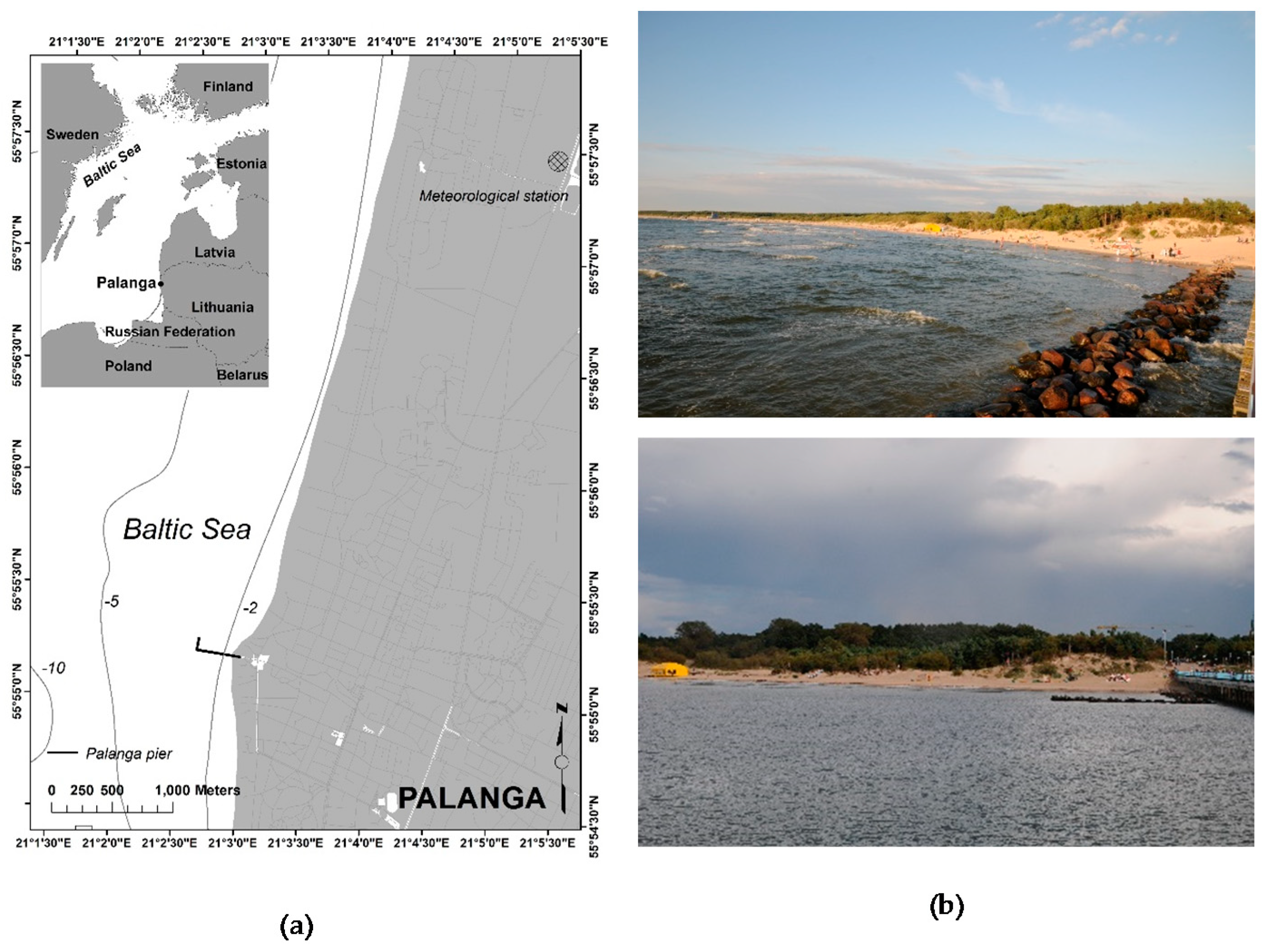
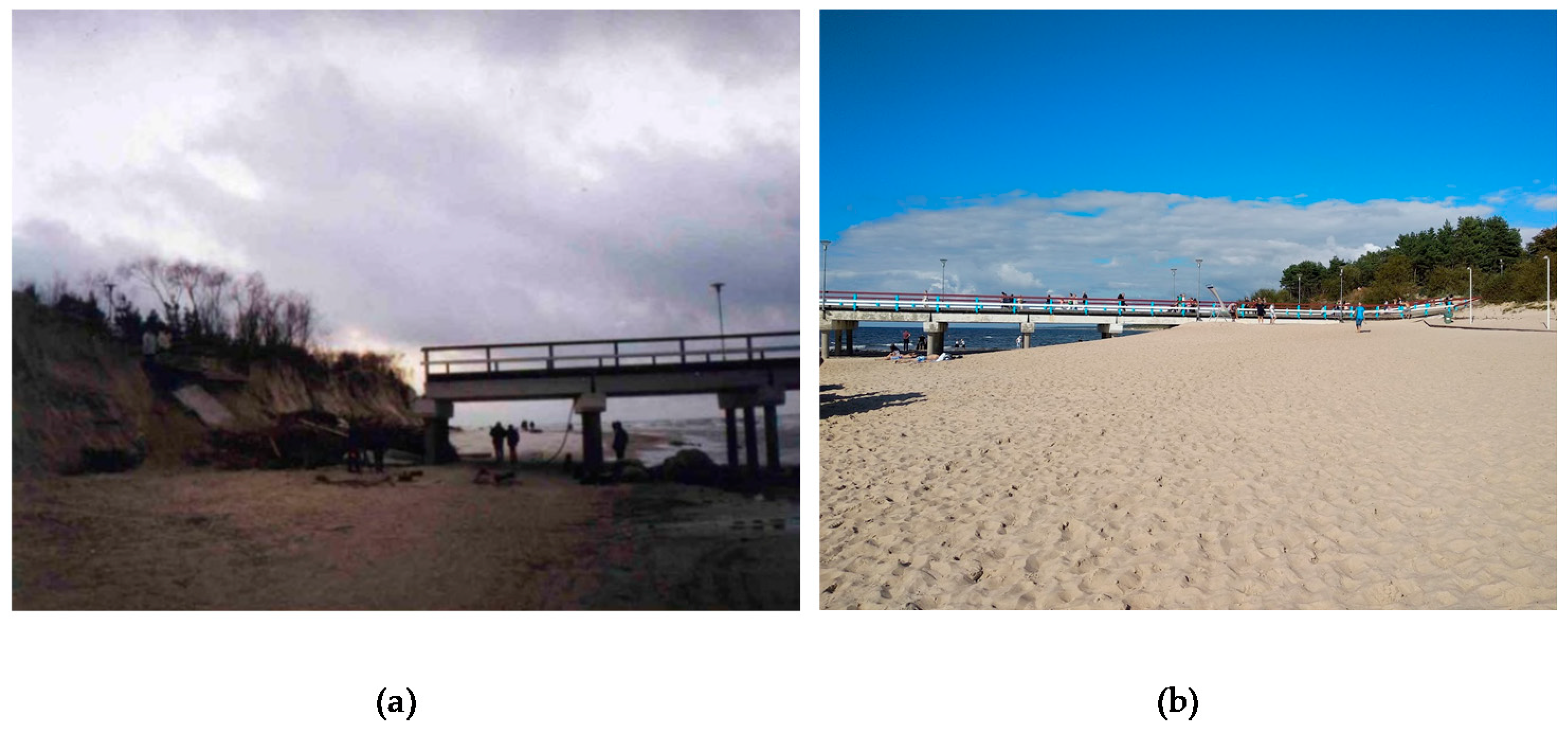
Cross-Shore Profile Evolution after an Extreme Erosion Event—Palanga, Lithuania

by
Loreta Kelpšaitė-Rimkienė
1,*,
Kevin E. Parnell
2,
Rimas Žaromskis
1 and
Vitalijus Kondrat
1
1
Marine Research Institute, Klaipėda University, 92294 Klaipėda, Lithuania
2
Department of Cybernetics, Tallinn University of Technology, 19086 Tallinn, Estonia
*
Author to whom correspondence should be addressed.
J. Mar. Sci. Eng. 2021, 9(1), 38; https://doi.org/10.3390/jmse9010038
Submission received: 1 December 2020 / Revised: 19 December 2020 / Accepted: 22 December 2020 / Published: 2 January 2021
(This article belongs to the Special Issue Coastal Morphology Assessment and Coastal Protection)

Abstract

:
We report cross-shore profile evolution at Palanga, eastern Baltic Sea, where short period waves dominate. Cross-shore profile studies began directly after a significant coastal erosion event caused by storm “Anatol”, in December of 1999, and continued for a year. Further measurements were undertaken sixteen years later. Cross-shore profile changes were described, and cross-shore transport rates were calculated. A K-means clustering technique was applied to determine sections of the profile with the same development tendencies. Profile evolution was strongly influenced by the depth of closure which is constrained by a moraine layer, and the presence of a groyne. The method used divided the profile into four clusters: the first cluster in the deepest water represents profile evolution limited by the depth of closure, and the second and third are mainly affected by processes induced by wind, wave and water level changes. The most intensive sediment volume changes were observed directly after the coastal erosion event. The largest sand accumulation was in the fourth profile cluster, which includes the upper beach and dunes. Seaward extension of the dune system caused a narrowing of the visible beach, which has led to an increased sand volume (accretion) being misinterpreted as erosion

1. Introduction

Explaining changes to nearshore coastal profiles remains a challenge for coastal researchers, particularly where there is considerable alongshore sediment transport [1,2,3]. Changes to the underwater profile are frequently examined under controlled hydrodynamic conditions in wave flumes [4,5], with some studies incorporating the effects of structures [6]. There are numerous examples of beach profile datasets presented in the literature (e.g., [1,2,3,7,8,9,10,11]), which consider how beaches change in response to variability in wind and wave conditions, advancing understanding with the analysis of each new dataset collected under different conditions. This study examines beach changes at Palanga, Lithuania, a heavily modified beach on a tideless coast with significant longshore sediment transport.
The Baltic Sea’s eastern coast is a high-energy (for the Baltic Sea), actively developing coast with fine, highly mobile sediments [12,13]. Sediment transport is generally counter-clockwise along the entire south-eastern coast of the Baltic Proper [14,15] from the Sambian Peninsula to Kolka Cape [16]. Minor variations in the physical nature of the coast and human activities (such as ports and other structures) add complexity to the system’s evolution. For example, parts of the underwater slope along the Lithuanian and Latvian shores have boulders, pebbles, and coarse sand. At the same time, in other sections, such as along the Curonian spit, there are fine sands with well-developed bar systems. Only in a few places (the Curonian Spit and a short coastal section to the south-east of Kolka Cape) are there substantial quantities of fine sediment [17]. These coast sections are generally stable or accretionary.
By comparison, other parts of the SE Baltic proper coasts are generally erosive [12,18,19]. The most significant areas of coastal retreat are near the Ports of Klaipeda, Liepaja, Ventspils, and in the vicinity of other structures [18,19,20,21]. Shoreline retreat near the Port of Klaipeda has reached 0.75 m/year since 1947 [12,22]. Further north, near the Port of Liepaja, there has been shoreline retreat more than 150 m since 1935, a rate of almost 2.5 m/year, and near the Port of Ventspils, 2 m/year shoreline retreat has been reported [19]. At Palanga (Figure 1), the site of this study, erosion of 0.75 m/year has been reported in the literature [12]. While some areas have been eroding, the well-developed dune systems on the SE Baltic coast have accumulated a large volume of sand [23], in part the result of soft coastal protection such as dune planting [24]. Development of the dune system is well correlated with the amount of vegetation immediately landward of the active beach [25]. Nevertheless, sediments accumulated in the dunes act as protection for the coastal ecosystem, but the ongoing retreat of the shoreline signals a decrease in the amount of sediment transported on the underwater slope.
Coastal processes on beaches within semi-enclosed or enclosed seas can vary from those on open ocean shores [22]. Swell waves are almost non-existent. Mean wave height on the SE Baltic Seacoast is 0.6 m [26,27]. Highest waves occur from September to January when monthly mean wave height reaches 0.8 m [28], with the overall maximum values 6 m [26]. Waves tend to be a short period (mean wave period about 2.5 s [27,29]), meaning that profile closure depths are limited, and wave refraction occurs close to the beach. Processes that generate significantly elevated water levels [23], such as storm surge [24] and wave set-up [25], which in turn are strongly related to coastal erosion, are highly variable in space and highly localized in their effect. A large proportion of the wave energy flux to the coast occurs on a very few days of the year [26], meaning that the wind direction at the time of major storms is a significant determinant of the coastal change outcomes. Changes in the wind regime, and therefore extreme water levels and wave characteristics [27], may radically alter coastal processes [28]. Few coastal beach profile studies address enclosed-sea environments, where the process-response regimes differ from open-ocean beaches.
Palanga (Figure 1) is the biggest eastern Baltic Sea seaside resort [30]. The first timber pier was built in 1889. It has a solid construction, interrupting the natural hydrodynamics and sediment transport. As a result, by 1892, sand accumulation next to the pier meant that ships were no longer able to moor. The design was adapted to repurpose the pier for recreation and Palanga was developed as a holiday resort. From construction until 1910, the shoreline moved seawards by “500 steps” (~400 m), and through to 1947, it accreted another 100 m [31]. At the end of the 19th century, the coast nearby was relatively flat, but by the middle of the 20th century, the shoreline comprised a dune field 80–100 m wide with 6–8 m high dunes, with a sand volume of about 400 m3 per linear meter [32]. Over the course of a hundred years, the pier was reconstructed several times, without changing its basic structure. In 1990, a decision was made to build a new concrete pier, permeable to waves and sediments. The new pier was completed in 1995, and demolition of the old impermeable structure started. Coastal erosion was observed soon after the shore perpendicular groynes, which were part of the old design, were removed in 1997 [31,32]. Significant coastal erosion becomes evident after the storm “Anatol” on 4 December 1999.
Storm “Anatol” remains the most damaging storm recorded on the SE Baltic Sea coast [33,34] with predominant west and north-west wind directions, mean wind speed up to 22m/s, and maximum wind gusts reaching 40 m/s [33]. “Anatol” stands out as being unusual for the Lithuanian coast by its trajectory over the Baltic Sea [35] resulting in up to 40 m/s south and south-west winds. Several comparable storms have since crossed Baltic Sea, examples being Ervin (or Gudrun) in 2005 and Kiril in 2007 [36,37] but they were more hazardous on the NE Baltic Sea coast [31,38,39]. During the storm “Anatol”, more than 3 million m3 of sand were eroded from the Lithuanian Baltic Sea coast [34], which at Palanga caused a 35 m reduction in beach width [31] and resulted in the dune base moving inland by 10 m [11,31,32]. The pier was damaged at its landward end and detached from the shore (Figure 2a), and the dune system was destroyed [30]. As a result of the changes, the groyne system (Figure 1b) was rebuilt in May 2000 [32].
In this paper, we analyze beach underwater profile recovery after the storm “Anatol” and the groyne reconstruction and later profile evolution. While processes associated with erosion of the upper beach and the deposition of sand in the nearshore are relatively well understood, cross-shore sediment transport variations under-recovery conditions have received less attention. The overall aim is to examine cross-shore sediment transport variations under different accretive conditions, beginning with a significantly eroded underwater beach profile, using conventional profile analysis, but incorporating analysis of transport rates and attempting to identify different process sections of profile using cluster analysis.

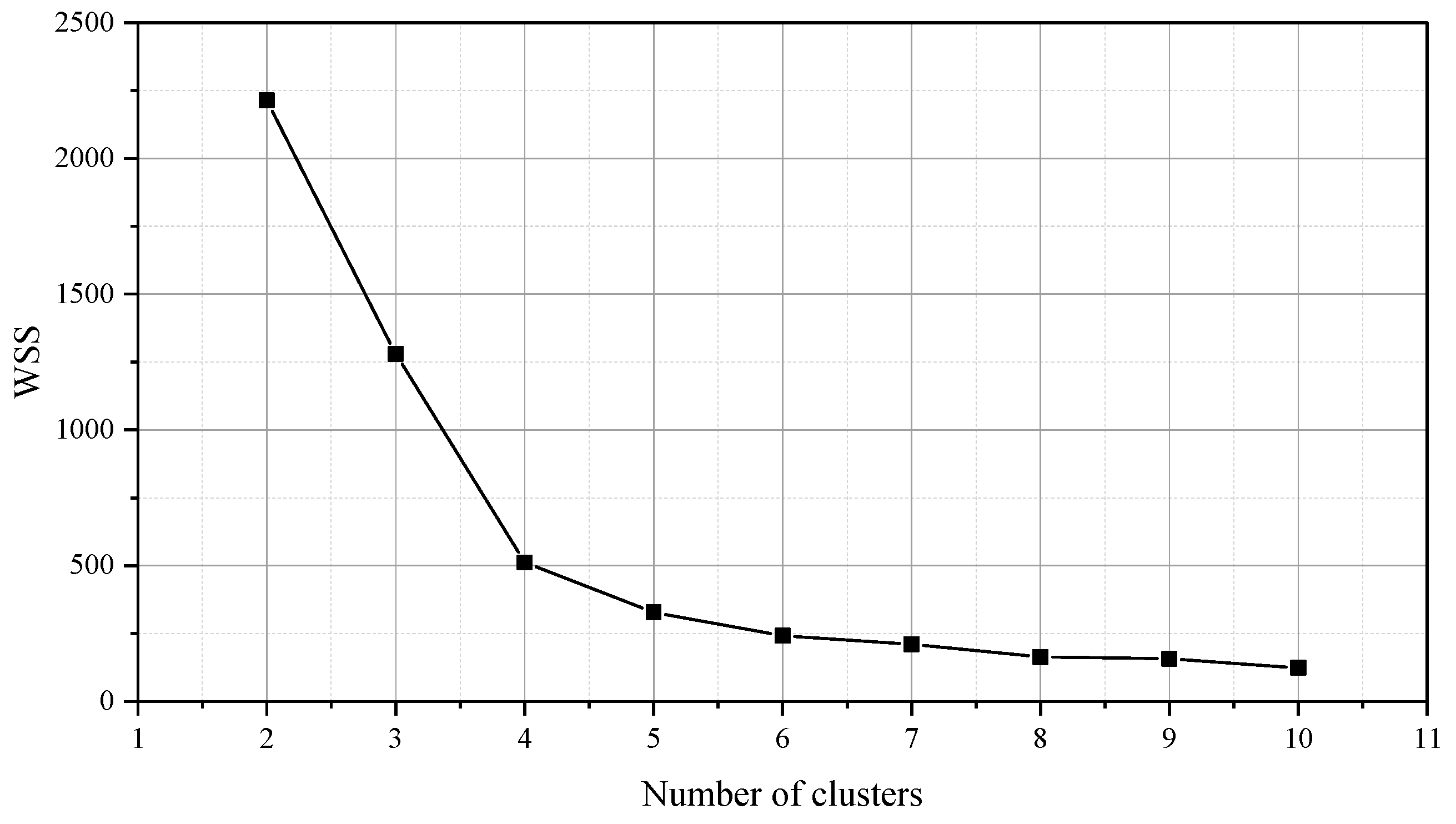
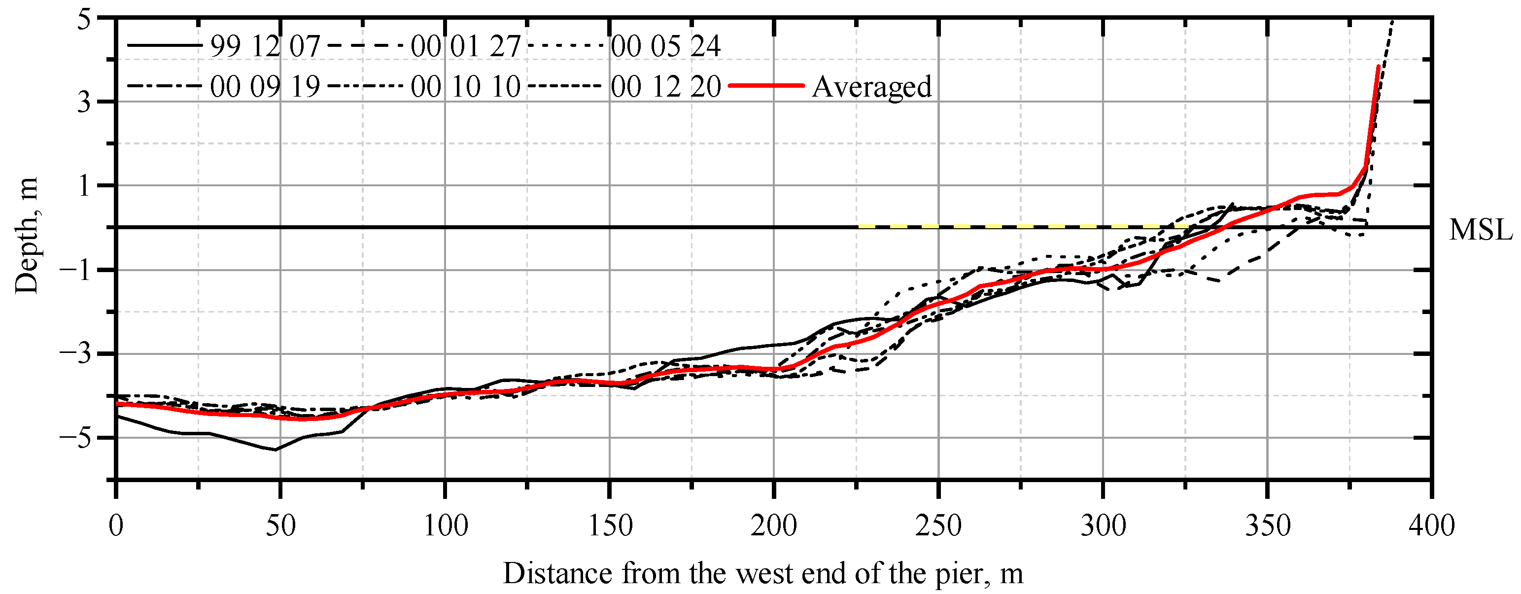
2. Materials and Methods

The cross-shore profile was surveyed at Palanga (Figure 1) adjacent to the Palanga pier over two time periods. The first set of measurements was undertaken in the period 1999–2000. Measurements began directly after the storm “Anatol” on 7 December 1999 and continued during the year 2000. Wind velocity and direction data for the study period were obtained from the Palanga hydro-meteorological monitoring station, Marine Research Department of the Environmental Protection Agency. Environmental monitoring was performed according to the national monitoring program guidelines prepared by the Lithuanian Ministry of Environment following various legal acts of the European Union [40].
Initially, the field experiment was designed to monitor cross-shore profile changes under different hydrometeorological conditions [11]. Sand composition on the underwater slope is characterized as well-sorted fine sands with a mean diameter of 0.18 mm [41]. Measurements with a weighted line (marked at 10 cm intervals) were made along the southern side of the pier (400 m length) every 2.5 m with zero distance being the pier’s seaward-most handrail. Although the water level on the coast oscillates with an amplitude of more than 1.5 m during storm surges [11], the apparent Mean Sea Level (MSL) is considered to be 5 m below the handrails, based on long-term observations. Measurements using the same methodology were undertaken in the stormy seasons of 2016 and 2017, with weekly measurements October–December until such time as there was ice along the coast.
The seaward limit of profile fluctuation over long-term (seasonal or multi-year) time scales is referred to as the “closure depth”, denoted by hc. Based on laboratory and field data, Hallermeier (1978, 1981) developed the first rational approach to determining closure depth [42]. Based on correlations with the Shields parameter, Hallermeier defined a condition for sediment motion resulting from relatively rare wave conditions. Effective significant wave height He and effective wave period Te were based on conditions exceeded only 12 h per year, i.e., 0.14 percent of the time. The resulting approximate equation for the depth of closure was determined to be:
h c = 2.28 H e 68.5 ( H e 2 gT e 2 )
H e = H ¯ + 5.6 σ H
h c = 2 H ¯ + 11 σ H
where g is gravity, and σH is the standard deviation of annual wave heights. Therefore, good approximation to the data is given simply by hc = 1.57 He [43]. In the case of the Lithuanian coast where He = 4 m [26], the depth of closure hc = 6.3 ± 0.5 m [43,44]. However, the storm “Anatol” revealed a layer of hard moraine sediments at ~−5 m depth, effectively constraining the profile at a level above calculated closure depth [11].
Comparative plots of beach profile evolution over time were constructed for the 1999–2000, 2016, and 2017 year cases. Average profiles for the periods were calculated. The cross-shore transport rates Q(x) were calculated using the methods in [4,5]. The total sediment transport rate (bedload and suspended load) per unit width between any two time periods (interval Δt) is determined from:
Q ( x n ) = Q ( x n 1 ) x n 1 x n ( 1 p ) Δ z b Δ t dx
where positive values of Q(xn) (m2/Δt) represent onshore sediment transport at position n, Δzb is the difference in the bed elevation between measurement intervals (m), Δt is the time difference between measurements (year), and p is the porosity of the sand, being 0.4 [2,5,9]. We assume no net sediment transport past the run-up limit xmax and beyond the depth of closure xmin, and sediment transport occurs consistently over the beach profile.
The bulk cross-shore sediment transport Q across the whole profile between any two time periods is determined by integrating the local transported volume along the profile [5]:
Q = Δ t x min x max Q ( x ) dx
between the same closure limits. Q represents the bulk cross-shore sediment transport (m3 per linear meter) moved either shoreward (positive) or offshore (negative). This measure has been used to categorize the overall beach response as erosive (Q < 0), accretionary (Q > 0) or stable (Q ≈ 0). Note that Q is a transport vector and can be either purely negative or positive, or a mixture, and therefore does not integrate to zero unless the onshore and offshore transport magnitudes are equal or both identically zero.
We use K-means clustering to determine clusters of cross-shore profile segments with similar development trends [45]. The K-means algorithm is one of the most popular hierarchical algorithms and uses the minimum sum of squares to assign observations to groups. Such groups of data points are called clusters [46,47]. Observations allocated to the closest cluster, and the distance between an observation and a cluster is calculated from the Euclidean distance between the observation and the cluster center. The objective function of K-means is given as:
E = | | X i m i | | 2
where: E is the sum of square error for all objects in the data, Xi is the point in a cluster, and mi the mean of cluster ki. The goal of K-means is to minimize the sum of the squares error over all k clusters. The algorithm states that, initially, k points are placed into space represented by objects that need to be clustered as initial group centroids. In the second step, each object is assigned to its closest cluster center. Then, the mean of each cluster is calculated to have a new centroid. These steps are repeated until there is no change in centroids. The number of clusters was selected based on the elbow method [45], the main idea of which is to define clusters such that the total intra-cluster variation (or total within-cluster sum of square (wss)) is minimized. As seen in Figure 3, the elbow of the curve is formed when the number of clusters is equal to 4.

3. Results

The most significant damage to the coast caused by hurricane “Anatol” was not a retreat of the shoreline, but a significant loss of sand from the protective dune ridge [48]. The cross-shore profile measured directly after the storm shows that significant volume of sand was lost from the underwater section of the beach, down to the effective closure depth of −5 m (Figure 4).
Further erosion was observed in the month following the first survey on 7 December 1999, under relatively calm meteorological conditions with maximum 13 m/s predominant SW (22%) and W (23%) winds (Figure 5b). A total of 66 m3 of sand per linear meter of shoreline was lost (Figure 6a(i)) in one month. The sand was moved from the −1.7 to −3.6 m depths to deeper than −4 m, covering the exposed moraine sediments. The position of MSL (0 m), moved landward by 20 m (Figure 6a(i)). The cross-shore sediment transport rate Q shows a bidirectional sediment transport tendency: shoreward at 0–180 m and seawards at 180–350 m resulting in accumulation of sand on the lower part of the profile (Figure 6b(i)).
From January to May 2000, there were several periods of strong wind with wind speeds up to 16 m/s, with westerly winds prevailing: 21% from W and 19% from SW directions (Figure 5c). These meteorological conditions led to coastal erosion: as a result, the groyne system (Figure 1b) was rebuilt [10]. Measurements in May 2000 showed that after the rebuilding of the groyne, 69 m3 of sand per linear meter was accumulated. The largest accumulation took place on the upper part of the profile between 215 and 325 m (Figure 6a(ii)). The cross-shore sediment transport volume across the whole profile from January to May was 5551 m2 with sand transport shoreward from the 218 m position (Figure 6b(ii)).
In summer (May–September 2020), calm weather prevailed (Figure 5d), and there was onshore transport. Almost the entire underwater profile shows positive Q transport, and, as a result, there was accumulation on the upper part of the profile, and the dune was partly replenished with sand (Figure 6a(iii)).The presence of the newly rebuilt groyne system, together with a calm autumn, extended a favorable condition for sand accumulation on the upper part of the cross-shore profile. September–December 2000 was calm with average wind speeds up to 12 m/s, with a predominant SE direction (Figure 5e,f). Profile changes showed sand movement from the shallow area to the offshore (Figure 6a(iv,v)), and in three months (October–December) only 7 m3 per linear meter of sand was lost on the underwater profile, with sand simply being relocated on the profile. It is noticeable that the cross-shore profile May–December was relatively stable and probably approximated the equilibrium profile shape for this location.
Profile measurements were repeated after 16 years with the expectation that perceptible erosion on Palanga beach [12,31,33,34,49,50] would be reflected in the underwater cross-shore profile. In addition, we expected to observe short-term changes in the cross-shore profile development during the stormy autumn season. Cross-shore profile measurements were repeated once per week in October–December 2016 and December 2017. Both measurement seasons were similar, with average wind speeds not exceeding 12 m/s. The significant difference between the two study seasons was in predominant wind direction: in 2016—N, E, and SE winds were prevalent, and in 2017—S, SW and W wind directions prevailed (Figure 7).
Over the sixteen years, 127 m3 per linear meter of sand accumulated on the cross-shore profile (Figure 8). Main changes were seen on the upper part of the profile, with the position of MSL moved seawards by 45 m. Net sediment transport rates were positive and indicated net sediment transport direction onshore. Dune expansion often creates the impression of beach narrowing and coastal erosion, which demonstrates the value of the data. Minor profile changes were seen in the deeper parts of the profile (perhaps indicating the real closure depth). Sediment was lost between 75 and 180 m with accumulation landward. The cross-shore sediment transport rate at a 75–300 m distance has negative values, showing a tendency for sand movement seawards. Sediment transport directed shoreward, Q, with positive values, is seen from 300 m. The sand accumulation zone starts from −4 m depth.
In 2016, changes in the cross-shore profile do not exceed 40 m3 per linear meter over one week. The sediment transport rate, Q, however, indicates considerable sand redistribution in the cross-shore profile without sand volume change (Figure 9). Noticeable changes in the profile shape were observed between 200 and 300 m and to −3 m depth. Small changes in weekly cross-shore profile volume show a quasi-stable state of the profile.
From December 2016 to October 2017, predominant wind directions were SW, NW, and W (Figure 7c). Wind speed did not exceed 12 m/s with the strongest winds from an E direction. Previous work [11] reported that westerly winds create favorable conditions for sand to remain on the underwater profile [11], but we observed sand loss under these conditions. In the relative calm and favorable wind direction conditions for accumulation, 36 m3 per linear meter of sand was eroded from location 200–300 m, between 0.5 m and −3 m depth (Figure 10a) and there was the retreat of the shoreline. In the dunes, some accumulation of sand occurred.
A bi-directional cross-shore sediment transport rate Q structure was seen at that time (Figure 10b). Onshore sediment transport direction (Q positive) was observed from 0 m to 245 m and offshore sediment transport (Q-negative) from 245 to 375 m. As a result, a bar was formed at −3 m depth.
Short-term profile changes and cross-shore sediment transport tendencies in 2017 were similar to those observed in autumn 2016. The sand bar formed at −3 m remained stable during the observation period (Figure 11a). We captured very small sand volume relocations on the profile. Sand movement on the cross-shore profile was mostly observed between the bar and mean sea level position; the largest sand relocations were observed close to the MSL position.
Total sand volume change during autumn 2017 was −30 m3 per linear meter, and the cross-shore sediment transport rate was ± 4356.1 m2 per week (Figure 11b). This tendency indicates sand relocation on the cross-shore profile without significant changes to the profile volume.
Seabed elevation changes in comparison with the average overall measured profiles indicate two different states (Figure 12). The seaward 130 m of the studied profile had minor changes in seabed elevation over 2016 and 2017. On more landward sectors, opposite trends were observed, being more active, with higher Δz values (up to ± 1 m). Only sectors greater than 300 m from the west end of the promenade bridge show positive Δz due to dune recovery after damage in December 1999.
To group cross-shore profile zones, K-means cluster analysis was performed. Cross-shore profile positions over the study period were grouped into four clusters, and all cross-shore profiles were also averaged. Standard deviations for the averaged curve were calculated (Figure 13).
The four clusters represent sectors on the cross-shore profile that change due to different conditions. The first cluster is the lower part of the profile from −5 m to 3.5 m and includes 38% of the total profile length (146 m). The deepest part of the profile is constrained by a moraine layer which is exposed in intense storms. Small scale seabed features result in minor (± 0.1 to ± 0.3 m) deviations from the average profile (Figure 14).
The second cluster comprises 114 m of the cross-shore profile, 30% of the length. It includes the middle section of the underwater profile from −3.5 m to −1.6 m depth. This part of the profile is above the depth of closure and falls into a more active hydrodynamic zone with more soft sediment than in deeper water. The standard deviation varies from ± 0.1 m to ± 0.8 m (Figure 14). The difference between the second and third clusters is likely the result of different hydrodynamic drivers. The second cluster is where waves and alongshore currents dominate most of the time, with the third cluster having similar process drivers, but affected by changes in the mean water level. This 73 m of the profile (19%) has a narrower distribution with standard deviation from ± 0.2 m to ± 0.7 m. The fourth cross-shore profile sector with the highest SD (from ± 0.2 m to ± 1.5 m), is the dune system, with different processes operating. It is the shortest cluster, just 49 m, with a height from 1.8 m to 3.2 m. The highest dune point was measured at 4.8 m in 2017.

4. Discussion

Beach profile features and evolution are essential considerations for coastal engineering projects. In the eastern Baltic Sea, profile dynamics have received comparatively less attention than alongshore processes, and the available knowledge remains partly qualitative and empirical [1,10,51,52,53,54].
Cross-shore profile evolution is often studied in a controlled environment such as in wave tanks [2,4,5,6], and results may be difficult to apply to realistic situations [9]. Often, the emphasis has been placed on the equilibrium profile for a particular location and the closure depth [51,55] but local geomorphological conditions (such as, in this case, the presence of a hard layer at −5 m) may be locally fundamental. In addition, interaction with structures on the coast may drastically change underwater beach profile evolution [6].
At Palanga beach, a quasi-equilibrium state [51] was reached in the hundred years after the promenade bridge was built [31,56]. This fragile state was destroyed in 1999 when a new pier, with an open design, was built [56], and substantial damage to the coast was done during storm “Anatol” [31,56]. Disruption of the quasi-equilibrium state created conditions that led to a new profile shape.
One storm, together with the new sediment transport conditions, changed the cross-shore profile and coastal zone characteristics enormously. Loss of sediment on the lower profile, deeper than −3 m, continued for another sixteen years. This area is further from the shoreline than the newly built groyne, but shallower than the depth of closure.
It is common practice to try to stop coastal erosion, using both soft (e.g., beach nourishment) and hard (e.g., wave breakers, groynes) coastal protection methods [57,58,59,60]. To stop further beach erosion, a groyne system was reconstructed in May 2000. First measurements after the groyne installation showed positive changes on the upper part of the profile. In sixteen years, 172 m3 of sand per linear meter was accumulated, with full dune system recovery. A narrowing of the beach occurred along with a foredune recovery [25,61,62]. The foredune will likely be eroded by waves when water levels with around a ten-year return period is reached, but it has had enough time to recover its long-term equilibrium shape [63]. Foredune recovery is a slow process that may take years to decades [64].
Part of the cross-shore profile corresponding to the dune sector falls into a separate fourth cluster, with the largest values of change and standard deviation. This section of the profile shows different development trends, dependent on the sediment characteristics rather than on the hydrometeorological conditions, which is intuitively predictable, but not statistically proven [61,63,64].
For the first cluster, close to closure depth, significant sediment relocation was observed after the storm “Anatol”. This area recovered fast, with insignificant (0.1–0.2 m) changes during most of the study period. Except during major storms there is little change on this deepest section of the profile due to the predominant short period waves in the SE Baltic Sea [61,63,64].
The rest of the profile was further divided into two parts, the second and third clusters. These sections of the profile behaved similarly, and the distribution of standard deviations fell within the same limits. We believe that the profile was separated into two sections due to predominant external forces (wave breaker, wave set-up, wave run-up and sea-level fluctuations) influencing the cross-shore sediment transport [51,65,66]. There is a need for additional studies to determine further which driving mechanisms dominate on which profile segment.
Comparison of cross-shore profiles in 2016 and 2017 show the importance of the direction of the predominant wind for profile evolution. Moreover, even a small change in the predominant wind direction from the south to the west caused opposite seabed elevation changes. This supports previous observations concerning the importance of the wind (and therefore wave) direction to Baltic Sea coastal evolution [12,15,26,67,68].

5. Conclusions

Three main conclusions regarding the cross-shore profile evolution at Palanga, eastern Baltic Sea coast, can be drawn from the results of this study. Firstly, the cross-shore profile is limited by a layer of hard moraine sediments which is exposed in intense storms. Secondly, intensive sediment relocation occurs at depths shallower than −4 m, where the wind (and therefore wave) direction and short-term sea-level fluctuations are critical to profile change. Thirdly, accurate beach profile data collection and analysis are essential because visual observations cannot be relied upon. It has been frequently stated that Palanga beach has been eroding in recent years, but apparent erosion, evidenced by a narrowing upper beach, is caused by dune advance.

Author Contributions

Methodology, R.Ž.; formal analysis, V.K.; investigation, L.K.-R., and V.K.; data curation, L.K.-R., and V.K.; writing—original draft preparation, L.K.-R.; writing review and editing, K.E.P.; visualization, V.K. All authors have read and agreed to the published version of the manuscript.

Funding

The APC was funded by the Baltic Research Programme (EEA Financial Mechanisms 2014-2021) project “Solutions to current and future problems on natural and constructed shorelines, eastern Baltic Sea” (EMP480). Parnell was also supported by the Estonian Ministry of Education and Research (Estonian Research Council, institutional support IUT33-3), and the European Regional Development Fund program Mobilitas Pluss MOBTT72, No. 2014-2020.4.01.16-0024.

Institutional Review Board Statement

Not applicable.

Informed Consent Statement

Not applicable.

Data Availability Statement

The data presented in this study are available on request from the corresponding author.

Acknowledgments

The authors would like to thank Emilija Griniūtė for assistance with data collection.

Conflicts of Interest

The authors declare no conflict of interest.

References

  1. Aagaard, T.; Hughes, M.G. Equilibrium shoreface profiles: A sediment transport approach. Mar. Geol. 2017, 390, 321–330. [Google Scholar] [CrossRef]
  2. Baldock, T.E.; Birrien, F.; Atkinson, A.; Shimamoto, T.; Wu, S.; Callaghan, D.P.; Nielsen, P. Morphological hysteresis in the evolution of beach profiles under sequences of wave climates—Part 1; observations. Coast. Eng. 2017, 128, 92–105. [Google Scholar] [CrossRef] [Green Version]
  3. Sanchez-Arcilla, A.; Caceres, I. An analysis of nearshore profile and bar development under large scale erosive and accretive waves. J. Hydraul. Res. 2017, 56, 231–244. [Google Scholar] [CrossRef]
  4. Baldock, T.E.; Alsina, J.A.; Caceres, I.; Vicinanza, D.; Contestabile, P.; Power, H.; Sanchez-Arcilla, A. Large-scale experiments on beach profile evolution and surf and swash zone sediment transport induced by long waves, wave groups and random waves. Coast. Eng. 2011, 58, 214–227. [Google Scholar] [CrossRef]
  5. Baldock, T.E.; Manoonvoravong, P.; Pham, K.S. Sediment transport and beach morphodynamics induced by free long waves, bound long waves and wave groups. Coast. Eng. 2010, 57, 898–916. [Google Scholar] [CrossRef]
  6. Beuzen, T.; Turner, I.L.; Blenkinsopp, C.E.; Atkinson, A.; Flocard, F.; Baldock, T.E. Physical model study of beach profile evolution by sea level rise in the presence of seawalls. Coast. Eng. 2018, 136, 172–182. [Google Scholar] [CrossRef] [Green Version]
  7. Austin, M.; Masselink, G.; O’Hare, T.; Russell, P. Onshore sediment transport on a sandy beach under varied wave conditions: Flow velocity skewness, wave asymmetry or bed ventilation? Mar. Geol. 2009, 259, 86–101. [Google Scholar] [CrossRef]
  8. Kobayashi, N.; Zhu, T.; Mallavarapu, S. Equilibrium beach profile with net cross-shore sand transport. J. Waterw. Port Coast. Ocean Eng. 2018, 144. [Google Scholar] [CrossRef] [Green Version]
  9. Patterson, D.C.; Nielsen, P. Depth, bed slope and wave climate dependence of long term average sand transport across the lower shoreface. Coast. Eng. 2016, 117, 113–125. [Google Scholar] [CrossRef]
  10. Roelvink, J.A.; Stive, M.F.J. Bar-generating cross-shore flow mechanisms on a beach. J. Geophys. Res. 1989, 94, 4785–4800. [Google Scholar] [CrossRef]
  11. Žaromskis, R. Impact of different hydrometeorological condition on Palanga shore zone relief. Geografija 2005, 41, 17–24. [Google Scholar]
  12. Bagdanavičiūtė, I.; Kelpšaitė, L.; Daunys, D. Assessment of shoreline changes along the Lithuanian Baltic Sea coast during the period 1947–2010. Baltica 2012, 25, 171–184. [Google Scholar] [CrossRef] [Green Version]
  13. Soomere, T.; Viška, M. Simulated wave-driven sediment transport along the eastern coast of the Baltic Sea. J. Mar. Syst. 2014, 129, 96–105. [Google Scholar] [CrossRef]
  14. Knaps, R. Sediment transport in the coastal area of the Eastern Baltic. In Development of Marine Coasts within the Conditions of Fluctuation Movements of the Earth Crust; Valgus: Tallinn, Estonia, 1966. [Google Scholar]
  15. Viška, M. Sediment Transport Patterns along the Eastern Coasts of the Baltic Sea; Tallin University of Technology: Tallinn, Estonia, 2014. [Google Scholar]
  16. Žaromskis, R.; Gulbinskas, S. Main patterns of coastal zone development of the Curonian Spit, Lithuania. Baltica 2010, 23, 146–156. [Google Scholar]
  17. Lapinskis, J. Coastal sediment balance in the eastern part of the Gulf of Riga (2005–2016). Baltica 2017, 30, 87–95. [Google Scholar] [CrossRef]
  18. Bagdanavičiūtė, I.; Kelpšaitė-Rimkienė, L.; Galinienė, J.; Soomere, T. Index based multi-criteria approach to coastal risk assesment. J. Coast. Conserv. 2018. [Google Scholar] [CrossRef]
  19. Eberhards, G.; Grine, I.; Lapinskis, J.; Purgalis, I.; Saltupe, B.; Toklere, A. Changes in Latvia’s seacoast (1935–2007). Baltica 2009, 22, 12. [Google Scholar]
  20. Bagdanavičiūtė, I.; Kelpšaitė, L.; Soomere, T. Multi-criteria evaluation approach to coastal vulnerability index development in micro-tidal low-lying areas. Ocean Coast. Manag. 2015, 104, 124–135. [Google Scholar] [CrossRef]
  21. Eberhards, G.; Lapinskis, J. Processes on the Latvian coast of the Baltic Sea. In Atlas; University of Latvia: Riga, Latvia, 2008; p. 64. [Google Scholar]
  22. Bagdanavičiutė, I.; Kelpšaitė, L.; Daunys, D. Long term shoreline changes of the Lithuanian Baltic Sea continental coast. In Proceedings of the 2012 IEEE/OES Baltic International Symposium (BALTIC), Klaipeda, Lithuania, 8–10 May 2012; pp. 1–6. [Google Scholar]
  23. Łabuz, T.A.; Grunewald, R.; Bobykina, V.; Chubarenko, B.; Česnulevičius, A.; Bautrėnas, A.; Morkūnaitė, R.; Tonisson, H. Coastal dunes of the Baltic Sea shores: A review. Quaest. Geogr. 2018, 37, 47–71. [Google Scholar] [CrossRef] [Green Version]
  24. Povilanskas, R.; Riepšas, E.; Armaitienė, A.; Dučinskas, K.; Taminskas, J. Shifting Dune Typesof the Curonian Spit and Factors of Their Development. Baltic For. 2011, 17, 215–226. [Google Scholar]
  25. Urboniene, R.; Kelpšaite, L.; Borisenko, I. Vegetation impact on the dune stability and formation on the Lithuanian coast of the Baltic sea. J. Environ. Eng. Landsc. Manag. 2015, 23, 230–239. [Google Scholar] [CrossRef]
  26. Kelpšaitė, L.; Dailidienė, I. Influence of wind wave climate change to the coastal processes in the eastern part of the Baltic Proper. J. Coast. Res. 2011, 64, 220–224. [Google Scholar]
  27. Soomere, T.; Räämet, A. Spatial patterns of the wave climate in the Baltic Proper and the Gulf of Finland. Oceanologia 2011, 53, 335–371. [Google Scholar] [CrossRef] [Green Version]
  28. Pindsoo, K.; Soomere, T.; Zujev, M. Decadal and long-term variations in the wave climate at the Latvian coast of the Baltic Proper. In Proceedings of the Ocean: Past, Present and Future—2012 IEEE/OES Baltic International Symposium, BALTIC 2012, Klaipėda, Lithuania, 8–11 May 2012. [Google Scholar]
  29. Suursaar, Ü.; Kullas, T. Decadal variations in waveheights off Cape Kelba, Saaremaa Island, andtheir relationships withchanges in wind climate. Oceanologia 2009, 51, 39–61. [Google Scholar] [CrossRef] [Green Version]
  30. Povilanskas, R.; Armaitienė, A. Seaside resort-hinterland Nexus: Palanga, Lithuania. Ann. Tour. Res. 2011, 38, 1156–1177. [Google Scholar] [CrossRef]
  31. Dubra, V. Influence of hydrotechnical structures on the dynamics of sandy shores: The case of Palanga on the Baltic coast. Baltica 2006, 19, 3–9. [Google Scholar]
  32. Jarmalavičius, D. Sea Coast Dynamics Next to the Palanga in Last Century. Available online: https://www.lrt.lt/naujienos/tavo-lrt/15/47235/d-jarmalavicius-juros-kranto-ties-palanga-kaita-per-paskutini-simtmeti-radijo-paskaita (accessed on 29 November 2019).
  33. Jarmalavicius, D.; Šmatas, V.; Stankunavicius, G.; Pupienis, D.; Žilinskas, G. Factors controlling coastal erosion during storm events. J. Coast. Res. 2016, 1, 1112–1116. [Google Scholar] [CrossRef]
  34. Jarmalavičius, D.; Satkunas, J.; Žilinskas, G.; Pupienis, D. Dynamics of beaches of the Lithuanian coast (the Baltic Sea) for the period 1993-2008 based on morphometric indicators. Environ. Earth Sci. 2012, 65, 1727–1736. [Google Scholar] [CrossRef]
  35. Ulbrich, U.; Fink, A.H.; Klawa, M.; Pinto, J.G. Three extreme storms over Europe in December 1999. Weather 2001, S56, 10. [Google Scholar] [CrossRef] [Green Version]
  36. Mäll, M.; Suursaar, Ü.; Nakamura, R.; Shibayama, T. Modelling a storm surge under future climate scenarios: Case study of extratropical cyclone Gudrun (2005). Nat. Hazards 2017, 89, 1119–1144. [Google Scholar] [CrossRef]
  37. Fink, A.H.; Brücher, T.; Ermert, V.; Krüger, A.; Pinto, J.G. The European storm Kyrill in January 2007: Synoptic evolution, meteorological impacts and some considerations with respect to climate change. Nat. Hazards Earth Syst. Sci. 2007, 9, 405–423. [Google Scholar] [CrossRef] [Green Version]
  38. Orviku, K.; Suursaar, Ü.; Tonisson, H.; Kullas, T.; Rivis, R.; Kont, A. Coastal changes in Saaremaa Island, Estonia, caused by winter storms in 1999, 2001, 2005 and 2007. J. Coast. Res. 2007, II, 1651–1655. [Google Scholar]
  39. Žilinskas, G. Distinguishing priority sectors for the Lithuanian Baltic Sea coastal management. Baltica 2008, 21, 85–94. [Google Scholar]
  40. Stankevičius, A. Conditions of the Baltic Sea environment; JTD, A., Ed.; AAA JTD: Vilnius, Lithuania, 2013. [Google Scholar]
  41. Žilinskas, G.; Pupienis, D.; Jarmalavičius, D. Possibilities of Regeneration of Palanga Coastal Zone. J. Environ. Eng. Landsc. Manag. 2010, 18, 92–101. [Google Scholar] [CrossRef]
  42. United States Army Corps of Engineers. CEM: Coastal Engineering Manual; U.S. Army Corps of Engineers: Washington, DC, USA, 2002. [Google Scholar]
  43. Soomere, T.; Viška, M.; Eelsalu, M. Spatial variations of wave loads and closure depths along the coast of the eastern Baltic Sea. Est. J. Eng. 2013, 19, 93–109. [Google Scholar] [CrossRef] [Green Version]
  44. Soomere, T.; Männikus, R.; Pindsoo, K.; Kudryavtseva, N.; Eelsalu, M. Modification of closure depths by synchronisation of severe seas and high water levels. Geo-Mar. Lett. 2017, 37, 35–46. [Google Scholar] [CrossRef]
  45. Laccetti, G.; Lapegna, M.; Mele, V.; Romano, D.; Szustak, L. Performance enhancement of a dynamic K-means algorithm through a parallel adaptive strategy on multicore CPUs. J. Parallel Distrib. Comput. 2020, 145, 34–41. [Google Scholar] [CrossRef]
  46. Steinley, D.; Brusco, M.J. Initializing K-means Batch Clustering: A Critical Evaluation of Several Techniques. J. Classif. 2007, 24, 99–121. [Google Scholar] [CrossRef]
  47. Melnykov, V.; Michael, S. Clustering Large Datasets by Merging K-Means Solutions. J. Classif. 2019. [Google Scholar] [CrossRef]
  48. Žilinskas, G.; Jarmalavičius, D.; Kulvičienė, G. Assessment of the effects caused by the hurricane ‘Anatoli’ on the Lithuanian marine coast. Geogr. Metraštis 2000, 33, 191–206. [Google Scholar]
  49. Jarmalavičius, D.; Žilinskas, G.; Pupienis, D.; Kriaučiuniene, J. Subaerial beach volume change on a decadal time scale: The Lithuanian Baltic Sea coast. Z. Geomorphol. 2017, 61, 149–158. [Google Scholar] [CrossRef]
  50. Pupienis, D.; Jarmalavičius, D.; Žilinskas, G.; Fedorovič, J. Beach nourishment experiment in Palanga, Lithuania. J. Coast. Res. 2014, 70, 490–495. [Google Scholar] [CrossRef]
  51. Dean, R.G.; Dalrymple, R.A. Coastal Processes with Engineering Applications; Cambridge University Press: Cambridge, UK, 2002. [Google Scholar]
  52. Miller, J.K.; Dean, R.G. A simple new shoreline change model. Coast. Eng. 2004, 51, 531–556. [Google Scholar] [CrossRef]
  53. Sousa, W.R.N.d.; Souto, M.V.S.; Matos, S.S.; Duarte, C.R.; Salgueiro, A.R.G.N.L.; Neto, C.A.d.S. Creation of a coastal evolution prognostic model using shoreline historical data and techniques of digital image processing in a GIS environment for generating future scenarios. Int. J. Remote Sens. 2018, 1–15. [Google Scholar] [CrossRef]
  54. Jara, M.S.; González, M.; Medina, R.; Jaramillo, C. Time-Varying Beach Memory Applied to Cross-Shore Shoreline Evolution Modelling. J. Coast. Res. 2018, 345, 1256–1269. [Google Scholar] [CrossRef]
  55. Dean, R.G. Equilibrium beach profiles: Characteristics and applications. J. Coast. Res. 1991, 7, 53–84. [Google Scholar]
  56. Žilinskas, G. Trends in dynamic processes along the Lithuanian Baltic coast. Acta Zool. Litu. 2005, 15, 204–207. [Google Scholar] [CrossRef]
  57. Gittman, R.K.; Fodrie, F.J.; Popowich, A.M.; Keller, D.A.; Bruno, J.F.; Currin, C.A.; Peterson, C.H.; Piehler, M.F. Engineering away our natural defenses: An analysis of shoreline hardening in the US. Front. Ecol. Environ. 2015, 13, 301–307. [Google Scholar] [CrossRef]
  58. Summers, A.; Fletcher, C.H.; Spirandelli, D.; McDonald, K.; Over, J.-S.; Anderson, T.; Barbee, M.; Romine, B.M. Failure to protect beaches under slowly rising sea level. Clim. Chang. 2018, 151, 427–443. [Google Scholar] [CrossRef] [Green Version]
  59. Armstrong, S.B.; Lazarus, E.D. Masked Shoreline Erosion at Large Spatial Scales as a Collective Effect of Beach Nourishment. Earth’s Future 2019, 7, 74–84. [Google Scholar] [CrossRef]
  60. Romine, B.M.; Fletcher, C.H. Hardening on eroding coasts leads to beach narrowing and loss on Oahu, Hawaii. In Pitfalls of Shoreline Stabilization: Selected Case Studies; Cooper, J., Andrew, G., Pilkey, O., Eds.; Springer Science and Business Media: Dordrecht, The Netherlands, 2012. [Google Scholar]
  61. De Almeida, L.R.; González, M.; Medina, R. Morphometric characterization of foredunes along the coast of northern Spain. Geomorphology 2019, 338, 68–78. [Google Scholar] [CrossRef]
  62. Jarmalavičius, D.; Pupienis, D.; Žilinskas, G.; Janušaitė, R.; Karaliūnas, V. Beach-Foredune Sediment Budget Response to Sea Level Fluctuation. Curonian Spit, Lithuania. Water 2020, 12, 583. [Google Scholar] [CrossRef] [Green Version]
  63. Pellón, E.; de Almeida, L.R.; González, M.; Medina, R. Relationship between foredune profile morphology and aeolian and marine dynamics: A conceptual model. Geomorphology 2020, 351. [Google Scholar] [CrossRef]
  64. Castelle, B.; Bujan, S.; Ferreira, S.; Dodet, G. Foredune morphological changes and beach recovery from the extreme 2013/2014 winter at a high-energy sandy coast. Mar. Geol. 2017, 385, 41–55. [Google Scholar] [CrossRef]
  65. Komar, P.D. Coastal erosion processes and impacts: The consequences of Earth’s changing climate and human modifications of the environment. Earth Syst. Environ. Sci. 2011, 285–308. [Google Scholar] [CrossRef]
  66. Komar, P.D. Beach Processes and Sedimentation; Prentice Hall: Upper Saddle River, NJ, USA, 1998. [Google Scholar]
  67. Viška, M.; Soomere, T. Simulated and observed reversals of wave-driven alongshore sediment transport at the eastern baltic sea coast. Baltica 2013, 26, 145–156. [Google Scholar] [CrossRef] [Green Version]
  68. Soomere, T.; Bishop, S.R.; Viška, M.; Räämet, A. An abrupt change in winds that may radically affect the coasts and deep sections of the Baltic Sea. Clim. Res. 2015, 62, 163–171. [Google Scholar] [CrossRef] [Green Version]
Figure 1. (a) Study area and (b) the northern side of the pier, with the adjacent groyne system (Photos: September 2018).
Jmse 09 00038 g001
Figure 2. (a) Palanga pier after the storm “Anatol”, December 1999, and (b) in September 2018.
Jmse 09 00038 g002
Figure 3. Within cluster sum of square dependence on the number of clusters.
Jmse 09 00038 g003
Figure 4. Changes in the beach profiles 1999–2000. The measurement date is indicated in the legend (yy mm dd); here and later, the yellow dash line indicates the length of the groyne.
Jmse 09 00038 g004
Figure 5. Wind roses for the study period: (a) 25 11 1999–06 12 1999; (b) 07 12 1999–26 01 2000; (c) 27 01 2000–23 05 2000; (d) 24 05 2000–19 09 2000; (e) 20 09 2000–09 10 2000; (f) 10 10 2000–19 12 2000.
Jmse 09 00038 g005
Figure 6. (a) Cross-shore profile changes (green-sand accumulation, red-sand loss) and (b) sediment transport rate Q, (i) December 1999–January2000, (ii) January–May2000, (iii) May–September 2000, (iv) September–October 2000, (v) October–December 2000.
Jmse 09 00038 g006
Figure 7. Wind roses for the October–December (a) 2016, (b) 2017 and (c) 2016 December–2017 October.
Jmse 09 00038 g007
Figure 8. Cross-shore profile changes (green-sand accumulation, red-sand loss) (a) and sediment transport rate Q (b) over the period 2000 to 2016.
Jmse 09 00038 g008
Figure 9. (a) Cross-shore profile changes (green-sand accumulation, red-sand loss) and (b) sediment transport rate Q in 2016.
Jmse 09 00038 g009
Figure 10. (a) Cross-shore profile changes (green-sand accumulation, red-sand loss) and (b) sediment transport rate Q, over the period 2016 to 2017.
Jmse 09 00038 g010
Figure 11. (a) Cross-shore profile changes (green-sand accumulation, red-sand loss) and (b) sediment transport rate Q, in 2017.
Jmse 09 00038 g011
Figure 12. Spatial and temporal evolution of bottom elevation changes (Δz) showing the average of all measured profiles (blue—2016, red—2017).
Jmse 09 00038 g012
Figure 13. Average of all measured profiles (red 1st, yellow 2nd, orange 3rd and green 4th clusters) with the standard deviation.
Jmse 09 00038 g013
Figure 14. Distribution (%) of standard deviation (sd) per the clusters (red 1st, yellow 2nd, orange 3rd and green 4th clusters).
Jmse 09 00038 g014
Publisher’s Note: MDPI stays neutral with regard to jurisdictional claims in published maps and institutional affiliations.

