Article

Resonantly Forced Baroclinic Waves in the Oceans: A New Approach to Climate Variability

by
Jean-Louis Pinault
Independent Scholar 1, 96, Rue du Port David, 45370 Dry, France
J. Mar. Sci. Eng. 2021, 9(1), 13; https://doi.org/10.3390/jmse9010013
Submission received: 2 December 2020 / Revised: 18 December 2020 / Accepted: 20 December 2020 / Published: 24 December 2020
(This article belongs to the Section Physical Oceanography)

Abstract

:
How variations in Earth’s orbit pace the glacial-interglacial cycles of the Quaternary are probably one of the greatest mysteries of modern climate science. These changes in the forcing are too small to explain the observed climate variations as simple linear responses. Consequently, to strictly apply the Milankovitch’s theory, a mediator involving positive feedbacks must be found, endowing the climate response with a resonant feature. This mediation should help explain the Mid-Pleistocene Transition (MPT) by involving orbital variations as the only external forcing, contrary to the current theory that supposes the coevolution of climate, ice sheets, and carbon cycle over the past 3 million years. Supported by both observational and theoretical considerations, recent work shows that long-period Rossby waves winding around subtropical ocean gyres meet the requirements of the sought mediator. Propagating cyclonically around the subtropical gyres, the so-called Gyral Rossby waves (GRWs) owe their origin to the gradient β of the Coriolis parameter relative to the mean radius of the gyres. The resulting modulated western boundary current, whose velocity is added to that of the steady anticyclonic wind-driven current, accelerates/decelerates according to the phase of GRWs. This amplifies the oscillation of the thermocline because of a positive feedback loop ensuing from the temperature gradient between the high and low latitudes of the gyres. Multi-frequency GRWs overlap, behaving as coupled oscillators with inertia resonantly forced by solar and orbital cycles in subharmonic modes. So, the efficiency of forcing increases considerably as the forcing period approaches a natural period of the GRWs. Taking advantage of (1) the alkenone paleothermometer in sediment cores sampled in the Tasman Sea floor, we show that, in the same way as during the MPT, but with periods 10 times longer, a transition occurred at the hinge of Pliocene-Pleistocene. Both transitions as well as the observed adjustment of the South Pacific gyre to the resonance conditions during the MPT are explained from orbital forcing alone—(2) data set of individual Globigerinoides ruber δ O   18 spanning the Holocene and the Last Glacial Maximum from sediment core in the eastern equatorial Pacific, we show how the El Niño–Southern Oscillation (ENSO) activity is modulated according to subharmonic modes. Periods of warming induce a decrease in ENSO activity while periods of cooling induce an increase.

1. Introduction

1.1. Background

1.1.1. The Mid-Pleistocene Transition (MPT)

While most climate transitions have been recognized as resulting from solar and orbital forcing due to their synchronism [1], understanding the underlying physical mechanisms is encountering considerable problems. Changes in the forcing are too small to explain the observed climate variations as simple linear responses [2]. Difficulties reach their culmination when the Mid-Pleistocene Transition (MPT) is considered, that is a fundamental change in the behavior of glacial cycles during the Quaternary glaciations. The transition happened approximately 1.2 million years ago, in the Pleistocene epoch. Before the MPT, the glacial cycles were dominated by a 41,000-year periodicity coherent with the Milankovitch forcing from axial tilt. After the MPT the cycle durations have increased, with an average length of approximately 100,000 years coherent with the Milankovitch forcing from eccentricity. However, the intensity of the forcing resulting from the eccentricity is much lower than that induced by the axial tilt.
Solar and orbital forcing of the climate system suggest that resonances occur, the forcing efficiency strongly depending on the periods. Over geological time, in addition to temperature variations, climate change has generated the deep transformation of the precipitation regime, the evolution of living species, and geological transformations resulting from glacial erosion as well as weathering processes. In return, the evolution of the terrestrial environment may have generated non-resonant feedback processes (the modification of the albedo in particular).
However, the cause and the effects of the resonant climate transition should not be confused. This has led some researchers to propose different mechanisms that can produce resonances. Stochastic resonance has been investigated, suggesting slow changes of climate are the integral response to continuous random excitation by short period disturbances [3,4,5,6,7,8,9]. This concept has been applied to large-scale, long-time sea surface temperature (SST) anomalies as the response of the oceanic surface layers to short-time-scale atmospheric forcing [10,11]. The role of stochastic freshwater forcing on the generation of millennial-scale climate variability in the North Atlantic has been studied using a coupled atmosphere–ocean–sea ice model [12,13,14,15,16,17]. These models are based on general principles and are more intended to propose amplification mechanisms than to explain precisely what is observed from climate records.
More precise models have been proposed to explain the MPT, involving long-term changes in atmospheric CO2 over the Quaternary [18,19,20,21]. A recent paper supposes the coevolution of climate, ice sheets, and carbon cycle over the past 3 million years [22]. It is assumed a decreasing level of atmospheric carbon dioxide, a high sensitivity to this decrease, and gradual removal of regoliths from northern hemisphere areas subject to glacial processes during the Quaternary. Regoliths are believed to affect glaciation: the base of ice on regolith at the pressure melting point will slide with relative ease, which limits the thickness of the ice sheet. This hypothesis suffers from an arbitrary condition that is the precise timing of the transition depending on the optimal regolith removal scenario prescribed additionally to orbital forcing. Without being able to justify the resonant nature of the climate system, this model requires an opportune adaptation of the Earth system to explain what is observed.

1.1.2. Long-Term Evolution of the El Niño–Southern Oscillation (ENSO)

The long-term driver of El Niño–Southern Oscillation (ENSO), i.e., the principal mode of interannual climate variability on Earth that is notable for both its large amplitude and global scope, remains largely hypothetical. Coral-based reconstructions from the tropical Pacific highlight long-term evolution of ENSO dynamics, especially valuable during the Holocene [23,24,25,26]. Island coral δ O   18 records reflect changes in SST as well as salinity. Uranium/thorium (U/Th)–dated fossil coral records spanning mid- and last Holocene show ENSO reduction between 4000 and 5000 years ago [27,28]. High-resolution record of surface radiocarbon reservoir ages for the southeast Australian region confirms the weakening of ENSO in mid-Holocene from paired radiocarbon ( C   14 ) and uranium series (U/Th) analysis of black corals, which are sensitive tracers of ocean circulation [29]. This is corroborated by (1) a biomarker rain gauge in the Galápagos Islands highlighting changes in the concentration and hydrogen isotope ratio of lipids produced by a green alga that blooms during El Niño rains in the Galápagos Islands [30] and (2) eastern tropical Pacific laminated sediments [31]. In the same way, quantitative precipitation record using carbon isotope ratios from a single species of leaf preserved in lake sediments from subtropical eastern Australia shows the reduction, between 5000 and 3000 years ago, of the Pacific Walker Circulation as contributing to the change in precipitations [32].
However, coral specimens older than 10,000 years are exceedingly rare, while information on ENSO evolution over glacial-interglacial cycles is of paramount importance to understand the long-term adjustment of geostrophic forces in the tropical Pacific Ocean. An alternative approach based on a surface-dwelling planktonic foraminifer from seafloor sediments allows long and continuous ENSO reconstructions from the ocean environment [33,34,35]. During their short life spans (about one month), shells of calcite (CaCO3) capture brief snapshots of SST and salinity in their oxygen-isotopic ratio ( δ O   18 ). Analysis of individual specimens prolific in the tropical oceans, deposited over narrow intervals of time, allows an estimation of the corresponding monthly variability. However, the set of specimens used for each snapshot of SST and salinity, whose number is necessarily limited to a few dozen, is not representative of the entire spectrum of states of the ocean environment. An accurate estimation of the variance of the oxygen-isotopic ratio would require several hundred samples because of the intrinsic variability of the amplitude of ENSO on the scale of a few decades. This is circumvented by increasing the frequency of snapshots for a long-term trend to emerge [35].
ENSO reconstructions from paleoclimate archives have fed interesting debates. However, the driver of ENSO remains enigmatic insofar as the only plausible forcing in the long term, which is the variation in solar irradiance, can only have an exceedingly small direct impact on ENSO.

1.2. Related Work

To strictly apply the Milankovitch’s theory to the long-term climate evolution, a mediator involving positive feedbacks must be found, endowing the climate response to variations in solar irradiance with a resonant feature. Referring to the recent theory of Gyral Rossby Waves (GRWs), approximately non-dispersive long-period Rossby waves winding around the subtropical ocean gyres meet the requirements of the sought mediator: with the mediation of GRWs the climate system preferentially responds to certain orbital variations according to subharmonic modes [36,37].

1.2.1. Short Period Rossby Waves

The way in which the concept of GRW is established derives from the observation and properties of short-period Rossby waves that are observable in the three tropical oceans where they are resonantly forced. They form Quasi-Stationary Waves (QSWs) from the equatorial Kelvin and Rossby waves and off-equatorial Rossby waves. QSWs are ruled by the forced version of linearized equations of motion (momentum, continuity, and conservation of the potential vorticity equations) whose solution highlights the resonance conditions [38,39,40].
Short period Rossby waves are also observable at mid-latitudes owing to the amplitude and phase of the cross-wavelet [41] of sea surface height (SSH) data obtained since 1992, scale-averaged within the bands 8–16 months, 3–6, and 6–12 years [42,43]. They clearly highlight the first 3 subharmonic modes whose 1-, 4-, and 8-year periods are inherited from the tropical QSWs via the western boundary currents. Short-period Rossby waves propagate westward but their phase velocity being lower than the velocity of the eastward propagating wind-driven current in which they are embedded, the apparent velocity of progressive Rossby waves is eastward. The western antinode is growing from where the western boundary current leaves the continent to re-enter the subtropical gyre while the poleward antinode is shrinking along the drift current (the circumpolar current in the southern hemisphere) before the SSH anomalies are reversed. Rossby waves owe their origin to the gradient β of the Coriolis parameter relative to the latitude [36].

1.2.2. Analogy between Short Period Rossby Waves and Gyral Rossby Waves

At the origin of the Atlantic Multidecadal Oscillation (AMO), GRWs are observable around the North and South Atlantic subtropical gyres owing to the amplitude and phase of the cross-wavelet of SST scale-averaged within the band 48–96 years [44]. Furthermore, in the North Atlantic, a GRW has been highlighted in the band 96–144 years by the same method. Thus, GRWs highlight subharmonic modes whose periods are 64 and 128 years. Propagating cyclonically, their phase velocity is lower than the velocity of the anticyclonic wind-driven current. So, the apparent velocity of progressive GRWs is anticyclonic. Now the internal antinode around the gyre is growing from where the western boundary current leaves the continent to re-enter the subtropical gyre while the external antinode is shrinking along the drift current before the SST anomalies are reversed. GRWs owe their origin to the gradient β of the Coriolis parameter relative to the mean radius of the gyre. They are ruled by the forced version of linearized equations of motion in polar coordinates. Indeed, whereas the β-plane approximation is used for solving equations relating to the short period Rossby waves, a β-cone approximation is required in the case of GRWs [44].
Since GRWs induce acceleration/deceleration of western boundary currents, they have a direct impact on climate cycles. So, the long periods of GRWs can be estimated indirectly from the climate archives [45]. Using paleothermometers in sediment cores sampled in ocean floor enables the observation over the last million years of the modulated currents of GRWs, which allows highlighting periods of several hundred years, or even several thousand/million years.

1.2.3. Properties of GRWs

But the analogy between short- and long-period Rossby waves ends there. Long-period Rossby waves have special properties resulting from their winding around subtropical gyres as their period increases.
Because of orbital forcing, a positive feedback loop involving the polar modulated current around the gyre occurs in response to the oscillation of the thermocline, which results from the temperature difference between low and high latitudes of the gyres: more heat being transferred from the tropics to the high latitudes of the gyres the thermocline deepens which, in turn, accelerates the western boundary current and vice-versa.
(1)
The progressive GRW must wind an integer number of turns around the gyre, over a half-wavelength. In this way the modulated polar and radial currents allow the warm water to accumulate around the gyre for a half-period, then to evacuate to the pole via the drift current (the circumpolar current in the southern hemisphere) during the following half-period.
(2)
GRWs do not dampen as their period increases because Rayleigh friction is compensated by the lengthening of the forcing duration. So, in theory, the periods of GRWs have no upper limit. Therefore, multi-frequency GRWs overlap, behaving as coupled oscillators because they share the same modulated polar and radial currents. Applied to the modulated currents of the subtropical gyres, the equations of motion of coupled oscillators with inertia require that GRWs are subharmonics of annual Rossby waves. Subharmonic modes ensure the durability of the resonant dissipative system, with each oscillator transferring as much interaction energy to all the others that it receives periodically [36]. Here the Caldirola–Kanai equation is used as the prototype of the equations of motion. It specifies how GRWs are resonantly forced by solar and orbital cycles in subharmonic modes. The natural period τ i of the i t h oscillator is an integer number of years deduced by recurrence: τ i = n i τ i 1 with τ 0 = 1 year, n i = 2 or 3 to ensure the stability of the gyres. Measurement of the apparent eastward velocity of 8-year period Rossby waves from their western antinodes (from where the western boundary currents leave the continents) allows estimating the time they would take to propagate all around the gyres (the phase velocity of long-period Rossby waves depends on the latitude of the centroid of the gyre, not on the period). Knowing that the very existence of such waves supposes that their period is a subharmonic of the fundamental wave, whose period is exactly one year as a result of the declination of the Sun, the time required to propagate around the gyre is 64 years for the North and South Atlantic, 128 years for the North and South Pacific and 32 years for the South Indian Ocean. It is convenient to deduce the period from the subharmonic modes using the North Atlantic as a reference. The first subharmonic mode being n 1 = 2 0 = 1 the corresponding period is n 1 × 64 = 64   years . Conversely, for a natural period τ i , the number of turns traveled in the North Atlantic is τ i / 64 . This also applies to the South Atlantic, but the number of turns is twice less in the North and South Pacific and twice more in the Southern Indian Ocean.
(3)
When the forcing period is close to the natural period of a GRW, a fine tuning occurs, resulting from increasing/decreasing of the mean radius of the gyre.
(4)
In the absence of the positive feedback resulting from the temperature gradient between the low and high latitudes of the gyres, the radial current ν would be in phase with solar irradiance (ν is positive outwardly of the gyre), the surface height perturbation η would be in quadrature with solar irradiance as well as the polar current υ (υ is positive when it is anti-cyclonic). The positive feedback has the effect of advancing the phase of GRWs by about a quarter of a period so that both the thermocline depth and the polar current velocity are nearly in phase with the forcing.

1.2.4. Subharmonic Modes

Contrary to the concepts exposed previously to explain the climate variability, that proposed here that is based on GRWs leads to constrained results, which reinforces its likelihood because having only an extremely low number of degrees of freedom. The only ones to be fixed being the two possible values of n i = 2 or 3, subharmonic modes are determined experimentally from the observed periods of GRWs. From periods extending from n 1 × 64 = 64 years ( n 1 = 2 0 ) to n 11 × 64 = 98.3 Ka ( n 11 = 3 × 2 9 ) they were deduced both from direct observation of Rossby waves along the ocean gyres, and from climate records. Indeed, as seen previously, the oscillation of the thermocline controls the polar and radial currents of the GRWs around the gyres, which accelerates/decelerates the western boundary currents. The resulting powerful positive feedback causes the GRWs to strongly impact the climate system.
The main modes are n 4 × 64 = 768 years ( n 4 = 3 × 2 2 ) that may trigger little ice ages during the Holocene, n 9 × 64 = 24,576 years ( n 9 = 3 × 2 7 ), n 10 × 64 = 49,152 years ( n 10 = 3 × 2 8 ), and n 11 × 64 = 98,304 years ( n 11 = 3 × 2 9 ) that contribute to glacial-interglacial cycles.

1.2.5. ENSO and the Equatorial Pacific

ENSO results from the coupling of an annual and a quadrennial QSW in the equatorial Pacific [42,43]. The annual QSW is formed by an equatorial first baroclinic, fourth meridional mode Rossby wave resonantly forced by easterlies. The quasi-geostrophic equilibrium of the tropical basin results in the modulated components of the North Equatorial Counter-Current (NECC) and the South Equatorial Current (SEC), both forming a single dynamical system [43]. The quadrennial QSW is formed from an equatorial first baroclinic mode Kelvin wave, and first baroclinic, first meridional mode equatorial, and off-equatorial Rossby waves [43]. Since they share the SEC, the annual and quadrennial QSWs are coupled. Consequently, they are resonantly forced in subharmonic modes, hence the 1-year and 4-year periods of QSWs.
The annual QSW being forced by easterlies its period is subject to low variability. By contrast, the period of the quadrennial QSW is very variable, being between 1.5 and 7 years. This is because the quadrennial QSW is partly self-sustained since forcing results from ENSO. The latter occur at the end of the eastward phase propagation of the quadrennial QSW. Evaporative processes induce the rise of the thermocline that initiates the recession of the equatorially trapped Rossby wave.
Transferring warm water from the western to the central-eastern tropical Pacific, a Kelvin wave initiates an ENSO event. This Kelvin wave is triggered by the annual QSW so that most of the ENSO events (81%) are in phase with the annual QSW, which means that they are mature between July and December when the eastward velocity of the modulated component of the SEC, that is, the southern node of the annual QSW, reaches its maximum. They are Eastern Pacific events (EP). By contrast Central Pacific events (CP) are out of phase with the annual QSW.
The QSW whose natural period is 4 years benefits from the geostrophic forces in the tropical basin. When ENSO events are in phase with the annual QSW (they occur during the second semester of the year), their conditions of formation are optimal every 4 years. Indeed, considering January 1998, 2002, ... as temporal milestones for the quadrennial cycle, 34% of ENSO events are unlagged since they occur in the interval (−0.5, 0 year) [43]. When ENSO events are out of phase with the annual QSW they are necessarily lagged since no event occurs in the interval (0, 0.5 year).
To summarize, whilst the mean frequency of the ENSO events is immutable, an event every 4 years on average, their distribution within the four-year cycles is subject to large variability, which may influence the intensity of events. On the other hand, the long-term dynamics of ENSO is controlled by the dynamics of the modulated components of the NECC and the SEC. Consequently, the geostrophic forces at the scale of the tropical basin, which are influenced by the subtropical gyres at low latitudes, must be considered in the evolution of ENSO.

2. New Clues in Favor of the Mediation of GRWs

The aim of this article is:
  • to extend the list of subharmonic modes in [45] to periods longer than 98.3 Ka while specifying the resonant nature of GRWs and their effects on climate. Taking advantage of the alkenone paleothermometer in sediment cores sampled in the Tasman Sea floor, we will show that, in the same way as during the MPT, but with periods 10 times longer, a transition occurred at the hinge of Pliocene-Pleistocene. Both transitions as well as the observed adjustment of the South Pacific gyre to the resonance conditions during the MPT will be interpreted as the response to orbital forcing of the climate system with the mediation of GRWs.
  • to find the driver of long-term ENSO evolution. Taking advantage of data set of individual Globigerinoides ruber δ O   18 spanning the Holocene and the Last Glacial Maximum from sediment core in the eastern equatorial Pacific, we will show how the ENSO activity is modulated according to subharmonic modes.
This will provide new clues in favor of the mediation of GRWs to explain the response of the climate system to orbital forcing, in a way to complement Milankovitch’s theory.

3. Materials and Methods

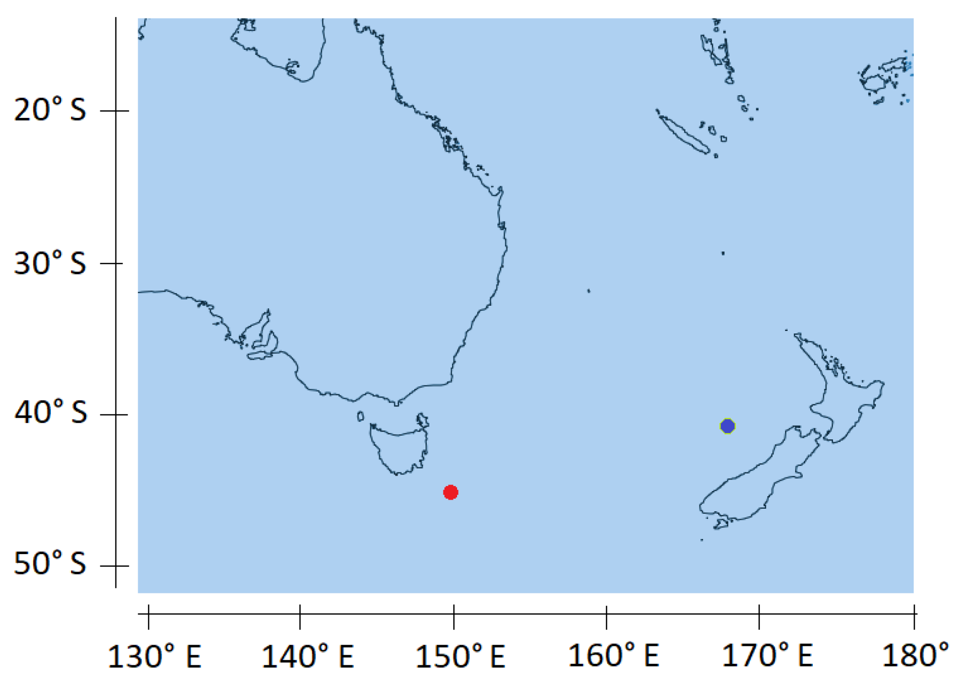
3.1. Sea Surface Temperatures at Deep Sea Drilling Project (DSDP) Site 593 and ODP Site 1172

SST at DSDP Site 593 (40°30′ S, 167°40′ E, 1068 m), presently situated north of the subtropical front, in the Tasman Sea [46], allows to extend subharmonic modes beyond what was explored previously due to the high resolution of the climate archive which spans 3.5 million years (Figure 1). Location of the DSDP Site 593 is favorable for the observation of the seawater temperature of the South Pacific gyre in its most southern part. It is indeed interpreted as evidence for varying influences of subtropical (warm) and sub-Antarctic (cold) waters in the southern Tasman Sea. Before 2.7 Ma, the warmer-than-present SSTs and overall low alkenone concentrations suggest that the subtropical front lay to the south of DSDP Site 593. These conditions are coeval with high abundances of nannofossil species characteristic of modern surface waters to the south of the subtropical front being recorded at ODP Site 1172 in the southwest Tasman Sea (44°57′ S, 149°55′ E, 2620 m) [47].
The optimal conditions are met for the study of the South Pacific gyre from observation of the subtropical front over time. Given the time scales, measurement of SST using the alkenone paleothermometer [46] in sediments (diagenetic product of chlorophyll) is not only representative of the SST but also of deeper waters. The main interest of this proxy is its sensitivity to temperature variations. Furthermore, it does not suffer from remanence phenomena as is the case for dissolved species due to exchanges with different reservoirs during diagenetic processes, which is detrimental to the time resolution.

3.2. Temperatures at DSDP Site 593 Compared to EPICA Data

Comparison of SST at DSDP Site 593 calibrated from alkenone concentration in sediment cores and EPICA temperature calibrated from Deuterium concentration in ice cores, both filtered in the band 73.7—47.5 Ka, shows that SST data are 1.25 lower than EPICA data. Comparison is carried out over 280 Ka BP, that is the time interval for which the time resolution of both series allows it.

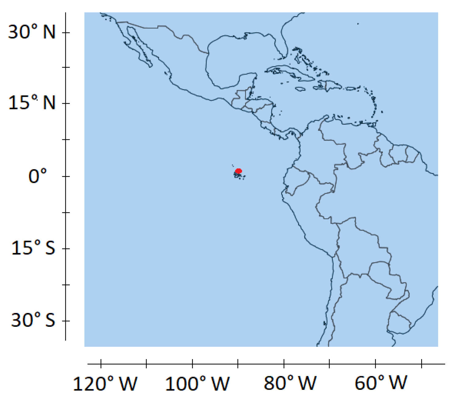
3.3. Variability of Individual Globigerinoides Ruber δ 18 O at Site V21–30

We use data set of individual Globigerinoides ruber δ O   18 spanning the Holocene and the Last Glacial Maximum from sediment core V21–30 in the eastern equatorial Pacific near the Galapagos Islands [35]. Core V21–30 (1°13′ S, 89°41′ W, 617 m depth) is located within the equatorial cold tongue formed by divergent upwelling that is reinforced during La Niña (Figure 2). This occurs during the westward phase propagation of the quadrennial QSW, in phase with ENSO [42,43]. The location of the drilling V21–30 experiences large SST anomalies correlated strongly with the Niño-3 index so that interpretation of G. ruber δ O   18 is framed primarily in terms of SST.

3.4. Data

Data referring to orbital variations calculated by Berger and Loutre, 1991 [48] are available at: https://www1.ncdc.noaa.gov/pub/data/paleo/climate_forcing/orbital_variations/insolation/orbit91.
Data referring to eccentricity and inclination variations calculated by Zeebe and Lourens, 2019 [49] are available at: https://www1.ncdc.noaa.gov/pub/data/paleo/climate_forcing/orbital_variations/zeebe2019orbital.txt.
Alkenone and benthic foraminiferal Mg/Ca paleothermometers at Deep Sea Drilling Project (DSDP) Site 593 in the Tasman Sea, southwest Pacific are available vs. time [46] at: https://www1.ncdc.noaa.gov/pub/data/paleo/contributions_by_author/mcclymont2016/mcclymont2016-dsdp593.txt.
100,000-year detailed oxygen isotope profile in Greenland Ice Sheet Project 2 (GISP2) ice core [50] is available at https://www.ncdc.noaa.gov/paleo-search/study/17796.
Deuterium data 2H obtained from Antarctica Dome C ice core (European Project for Ice Coring in Antarctica EPICA) are used for global mean temperature estimate in the southern hemisphere [51].
δ O   18 variance of individual G. ruber from the Holocene and Last Glacial Maximum calculated as the squared standard deviation of individual δ O   18 in each sample comes from [35].
Niño 3.4 SST Index [52] is available at https://www.psl.noaa.gov/gcos_wgsp/Timeseries/Nino34/.

3.5. Filtering

Since the wavelet transform is a bandpass filter of uniform shape and varying location and width, filtering time series in predetermined bands is performed by summing over a subset of the scales the wavelet functions. On the other hand, the variance of the Niño3 SST index within bands is obtained by scale-averaging the wavelet power over those bands. Here the Morlet wavelet consisting of a plane wave modulated by a Gaussian is used so that the scale and the period are confused [41].

4. Results and Discussion

4.1. The South Pacific Subtropical Gyre during the MPT

Why the insolation variations and their effects observed on the temperature of sea water at high latitudes of the gyres are not proportional stems from the efficiency of resonant forcing of GRWs in subharmonic modes, which depends on the deviation between the forcing and natural periods [45]. However, the relevance of GRWs is not only worthy of interest in the analysis of the causes of the MPT, but also for explaining the observed modifications of the circumference of the South Pacific subtropical gyre following this event whose impact is considerable. For this, the Tasman Sea is rich in observations, being subject to both the warm subtropical front and the cold sub-Antarctic front of the Antarctic Circumpolar Current. The history of currents over the last million years is traced through sediment cores sampled from the ocean floor within ocean deep drilling programs.
The evolution of the period of eccentricity over a few million years BP is deduced from orbital calculations [47]. Because it is subject to a large variability, the Fourier spectra are averaged over 1 Ma (Figure 3a), which results from a compromise between time and frequency resolution. Despite this time averaging, the Fourier transform has a spread maximum which is not conducive to determining the orbital forcing frequency with precision. The Fourier spectrum being approached by a parabola near its maximum, the latter is estimated analytically. It should be noted that the results obtained do not depend on the orbital variations calculated by two authors. As the Figure 3b shows, evolution of the periods of eccentricity over time is comparable, whether it is calculated from [47] or [49] although nearly three decades have elapsed between the two publications. From 1.2 Ma, the two periods frame the resonance period.
On the other hand, the integration over intervals of 1 Ma of the period requires that its representation as a function of time is deconvoluted. A solution is shown in Figure 3c, the one that is as smooth as possible to be the more realistic. Performing a moving average over 1 Ma of the solution allows faithfully reconstructing the initial period vs. time (Figure 3d).
According to Figure 3c the period of eccentricity varies greatly over the last 4 million years, approaching the period of resonance of the subharmonic mode n 11 , namely 98.3 Ka, since 1.2 Ma BP. The forcing efficiency related to that period has been increasing steadily since 1.4 Ma BP to reach 5 °C (W/m2)−1 at present, which suggests that the tuning is still improving [45] (the efficiency being obtained from EPICA proxies, the value of 4 °C (W/m2)−1 must be considered to be compared with the SST data).
A natural period of the GRWs becoming close to the forcing period, the gyres adjust to perfect the tuning between both periods. While the dominant period of the glacial-interglacial cycles before the MPT was 41 Ka, coherent with the obliquity, it has since been coherent with that of eccentricity although the amplitude of the orbital forcing is much higher for the obliquity than for the eccentricity.
The assumption that the GRWs were tuned to different forcing periods before and after the MPT assumes that the dominant period was 41 Ka before the MPT, as attested by the climate records. However, the closest natural period corresponds to the subharmonic mode n 10 , namely 49.2 Ka. The transition of the period from 41 Ka, when the subharmonic mode n 10 was tuned to the forcing period before the MPT, to the natural period of 49.2 Ka at present requires an adjustment of the gyre.
As the dispersion relation shows [36], lengthening of the period requires either an equatorward shift of the centroid of the gyre or an increase in its circumference. In the first case, the latitudinal displacement of the centroid increases the cyclonic phase velocity for an observer dragged along the wind-driven circulation but reduces the apparent anticyclonic phase velocity for a fix observer. In the second case, increasing the circumference lengthens the period since the phase velocity remains unchanged.
Considering together paleothermometers at DSDP Site 593 and ODP 1172, it is inferred that, during late Pliocene, a poleward displacement of the subtropical front compared to modern occurred between 40 and 44° S [46]. Consequently, the second hypothesis is the correct one. A 4° drift of the subtropical front towards the south without displacement of the centroid of the gyre increases the circumference by almost 20%, which reflects the adjustment of the gyre to increase the natural period of the subharmonic mode n 10 from 41 to 49.2 Ka. In this way, the drift of the subtropical front concomitantly with the MPT confirms the hypothesis that the latter results from bringing closer the natural period of the subharmonic mode n 11 , namely 98.3 Ka and the forcing period resulting from eccentricity variations.

4.2. Subharmonic Modes

When used as a proxy of SST (Figure 4a), alkenone concentration in sediment cores at DSDP Site 593 allows to accurately extend the properties of four subharmonic modes from n 12 to n 15 . As shown in Figure 4b the Fourier transform (FT) of SST vs. time highlights the periods of the main oscillations, that is, 218, 476, and 1131 Ka. However, analysis of the coherence between the variations in the total solar irradiance (TSI) resulting from orbital forcing and SST obliterates the peak at 218 Ka: only two peaks, one at 440 Ka and the other at 1046 Ka are visible (Figure 4e), which suggests an effective orbital forcing in this case.
It turns out that the peak at 218 Ka is close to the period corresponding to the subharmonic mode n 12 = ( 3 × 2 9 ) × 2 = 3 × 2 10 = 3072 , namely 3072 × 64 = 196.6 Ka. Since this peak does not appear in the coherence spectrum (Figure 4e), the period must be considered as a pure harmonic of longer periods (the coherence spectrum between two series varies from 0 to 1, the maximum value being reached between two sinusoids of the same period, in a bandwidth of infinite width).
In the coherence spectrum, the two peaks highlight the forcing from variations in eccentricity, the only orbital parameter whose period exceeds 41 Ka (Figure 4d). The first refers to the subharmonic mode n 13 = ( 3 × 2 10 ) × 2 = 3 × 2 11   =   6144 whose period is 6144 × 64 = 393.2 Ka. It appears that the mode for which the period is closest to the second peak is n 14 = ( 3 × 2 11 ) × 3 = 3 2 × 2 11 = 18 , 432 whose period is 18,432 × 64 =1180 Ka.

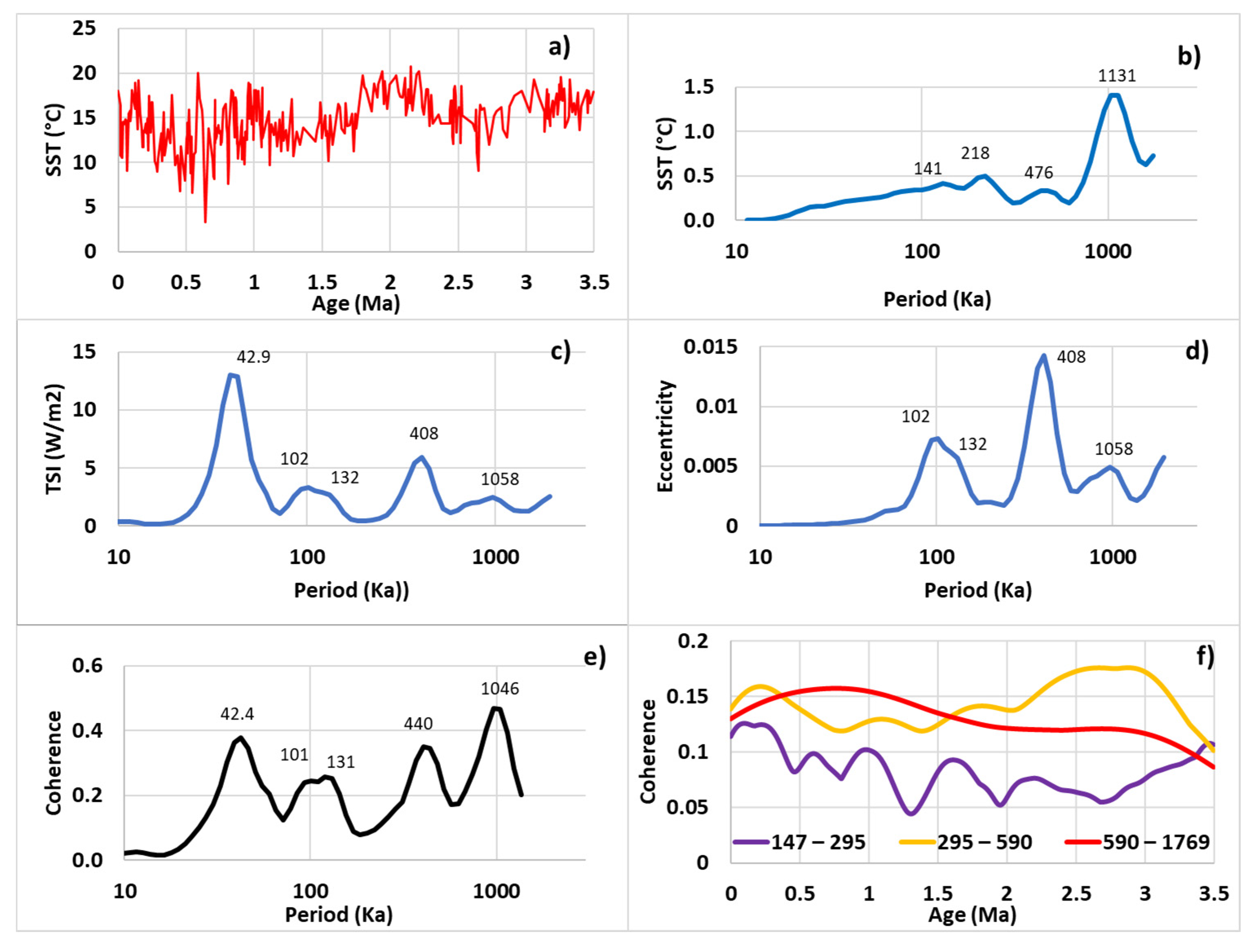
4.3. The Band 295–590 Ka

Comparison of TSI and de-trended SST filtered into the band 295–590 Ka characteristic of the subharmonic mode n 13 (Table 1, Figure 5) confirms that they are coherent because they are nearly in phase, a prerequisite for supporting a causal relationship between forcing and its presumed effects on subtropical ocean gyres [37]. However, the forcing efficiency varies over time since the oscillation of the SST weakens between 1.6 and 2.4 Ma BP while the forcing remains sustained throughout the observation period. Indeed, Figure 5b confirms the weakening of the forcing efficiency despite the vicinity of forcing and natural periods, that is, 408 and 393.2 Ka.

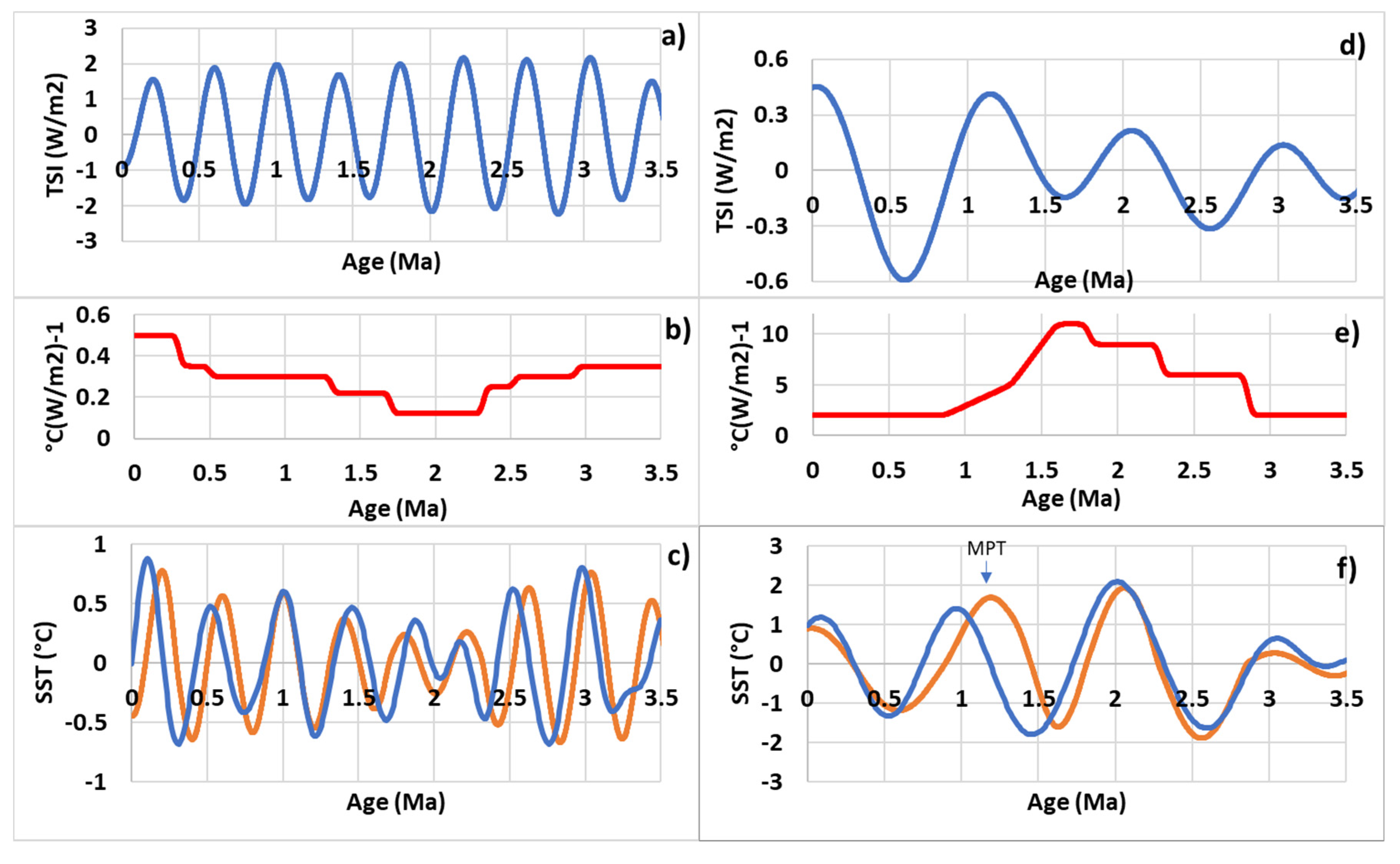
4.4. The Band 590–1769 Ka

As in the band 295–590 Ka, comparison of TSI and de-trended SST filtered into the band 590–1769 Ka characteristic of the subharmonic mode n 14 shows that they are nearly coherent, apart from the small phase shift which occurred between 1.5 and 0.8 Ma BP. This might reflect the adjustment of the gyre during the MPT (Figure 5f). As shown in Figure 5e the forcing efficiency increases considerably during the transition Pliocene-Pleistocene, overreaching 10 °C (W/m2)−1. Such a value denotes an optimum tuning between the natural and the forcing periods. The mode n 13 is multiplied by 3 to obtain the mode n 14 instead of 2: this reflects the strong influence of the forcing resulting from the eccentricity variations.

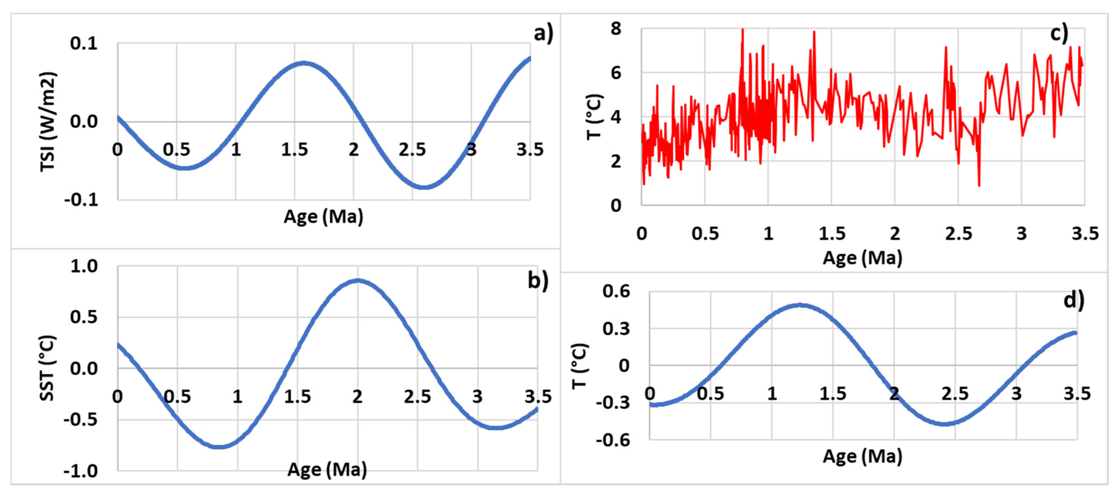
4.5. The Band 1769–3539 Ka

Due to the limitation imposed by the observation period, the investigated bandwidth is 1769–3500 Ka, which does not enable the FT of the series. SST filtered into this band (Figure 6b) exhibits an oscillation whose period is estimated nearly 2.27 Ma (half-period between 0.877 and 2.01 Ma). This period corresponds to the subharmonic mode n 15 = ( 3 2 × 2 11 ) × 2 = 3 2 × 2 12 =   36 , 864 whose natural period is 36,864 × 64 = 2359 Ka. This time, it is probably a pure subharmonic because de-trended SST and TSI filtered into this band are out of phase (Figure 6a,b).
Benthic foraminiferal Mg/Ca analysis at DSDP Site 593 is another paleothermometer: given the residence times of Mg (~14 Ma) and Ca (~1 Ma), the ocean temperature reconstructions from the Mg/Ca ratio is subject to a low band-pass filter (Figure 6c,d) so that the 1.08 Ma period oscillation disappears to the benefit of the longer period oscillation that refers to the subharmonic mode n 15 . It not only has the effect of filtering the high frequencies but also of delaying the phase of the oscillation by about 0.7 Ma while attenuating its amplitude. However, this allows the accurate estimation of the half-period between 1.24 Ma and 2.43 Ma, which estimates the period close to 2.38 Ma even more convincingly because here only one oscillation is isolated.

4.6. The Mid-Pleistocene and Pliocene-Pleistocene Transitions

A resonance phenomenon comparable to what is observed during the MPT occurs at the hinge of the Pliocene and the Pleistocene. This is illustrated in Figure 7, the only difference with Figure 3 being that, here, the periods are 10 times higher than previously. This requires the FT is performed on successive intervals of time of 2500 Ka instead of 1000 Ka (Figure 7a). Time intervals overlap to represent the period vs. time.
Whether it is Mid-Pleistocene or Pliocene-Pleistocene transition, two subharmonic modes are forced simultaneously. They are n 10 and n 11 whose natural periods are 49.2 and 98.3 Ka during the first transition, and n 13 and n 14 whose natural periods are 0.39 and 1.18 Ma during the second. The natural period of the highest mode tunes transiently, but optimally, to the forcing period when both become very close (Figure 3c and Figure 7c). Here again it must be noted that the results obtained do not depend on the orbital variations calculated by the two authors [47,49] as shown in Figure 7b. Then, the two subharmonic modes swap the dominant mode, as attested by the nearly symmetrical opposite variation in the forcing efficiencies (Figure 5b,e). The forcing efficiency of the higher mode exceeds 10 °C (W/m2)−1 between 2.4 and 1.6 Ma BP when the tuning is optimal whereas that of the lower mode drops to 0.12 °C (W/m2)−1. The change in the dominant period occurred approximately 2.2 Ma ago when the 0.39 Ma period oscillation collapsed in favor of the 1.18 Ma period oscillation (Figure 5c,f). Nowadays the transition is occurring in the other direction since the 1.18 Ma period oscillation is collapsing in favor of the 0.39 Ma period oscillation, both having approximately the same amplitude. This transition involves a weak adjustment in the circumference of the gyre because the deviation between the forcing and natural periods of the lower subharmonic mode is small, 0.41 and 0.39 Ma, respectively (Table 1, Figure 4c,d).

4.7. Long-Term Evolution of ENSO
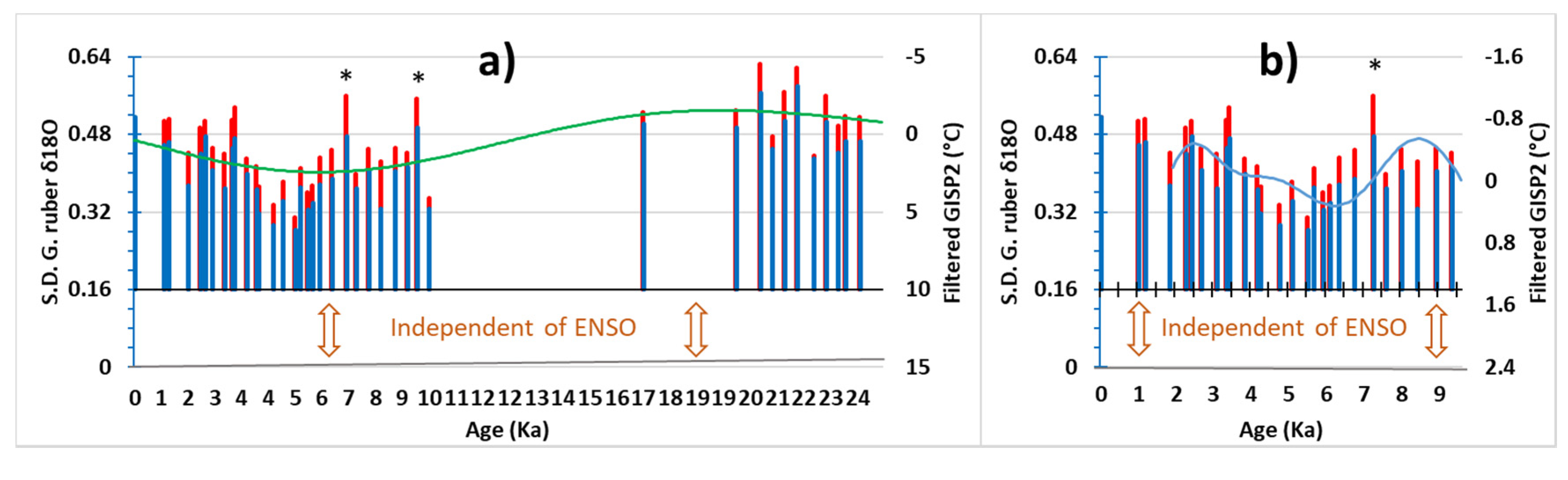
4.7.1. Standard Deviation of δ 18 O in Individual Globigerinoides ruber

Based on the variability of the equatorial Pacific in the 1.5–7 years band, highlighting the evolution of ENSO activity on the scale of a few thousand years is a challenge. The eastern equatorial Pacific within the equatorial cold tongue formed by divergent upwelling offers opportunities since it is strongly impacted by both warm El Niño and cold La Niña events.
δ O   18 concentrations in short-lived individual G. ruber [35] are proxies of monthly SSTs. Because of the investigated area, they are expected to be representative of the Nino3.4 index, i.e., the monthly SST anomalies averaged over the region 5 S-5 N and 170–120 W. Their standard deviation (Figure 8) reflects the evolution of ENSO activity during both the Holocene and the Last Glacial Maximum, which represents a substantial advance over previous work on isotopic analysis of corals that is generally limited to the Holocene. Indeed, to be determined with certainty, the dynamics of ENSO must be demonstrated for periods covering the widest possible range of subharmonic modes.
The standard deviations are subject to long-term variability at the scale of both the sampling interval, i.e., around 1 Ka where the measurements are the densest, and several thousand years. Their variations at the 1 Ka scale are difficult to interpret because of their large dispersion due to the small number of G. ruber involved. Assuming the independence of errors of standard deviations, their variations at the scale of several thousand years are expected to reflect the long-term evolution of the ENSO activity.
Thus, using δ O   18 in individual G. ruber as a proxy of the monthly Nino3.4 index, the part of the variance of the explanatory signal of ENSO in the band 1.5 to 7 years has to be estimated. The total variance of the Nino3.4 index from 1870 to 2020 [52] is 0.785 °C2 and the variance in the band characteristic of ENSO is 0.360 °C2 so that the part of the total variance referring to ENSO is 45.8% (for information, the part of the variance in the band 0.5 to 1.5 years characteristic of the annual variability is 30.1%). By assuming that most of the long-term variations of the estimated standard deviation S ( t ) (considered as a function of time t ) of G. ruber δ O   18 reflect the evolution of the ENSO activity, the invariant residual part is S ( t ) ¯ × ( 1 0.458 ) 0.16 where S ( t ) ¯ is the mean of S ( t ) (Figure 8).

4.7.2. Hydrological Processes

The only way to influence the long-term ENSO activity is to involve any interaction between the modulated geostrophic currents of the equatorial Pacific and those of the subtropical gyres, that is, the only source of variability of subsurface water (down to the thermocline) at the scale of orbital cycles. As already stated, the global temperature filtered in the characteristic bands of subharmonic modes can be used as a proxy of the amplitude of GRWs.
In Figure 8, the interactions of modulated geostrophic currents between the North Pacific gyre and the equatorial Pacific are materialized by comparing the activity of ENSO to the global temperature filtered in relevant bands as proxies of the amplitude of multifrequency GRWs around the North Pacific gyre. The global temperature of the Earth is obtained from the GISP2 ice core 110,000 year δ O   18 record [50]. In Figure 8a, the GISP2 δ O   18 record is filtered in the 18.4—36.9 Ka band characteristic of the subharmonic mode n 9 ( T = 24.6 Ka). This mode is considered as a pure harmonic of the modes n 10 and n 11 : orbital forcing that results from the variations in precession, whose period is close to that of the subharmonic mode n 9 , is very weak [45]. In Figure 8b the GISP2 δ O   18 record is filtered in the 2.3–4.6 Ka band characteristic of the subharmonic mode n 6 ( T = 3.1 Ka), which is a pure harmonic of higher modes, in order to focus on the interactions of modulated geostrophic currents between the North Pacific gyre and the equatorial Pacific during the Holocene.
Although the proxy of ENSO activity reflects a broad spectrum of hydrological variability, trends are emerging [35], disclosing that the long-term evolution of ENSO is negatively correlated to the filtered GISP2 signal. This means that geostrophic forces act on the NECC to enable reduction of the ENSO activity when the modulated polar current of the North Pacific subtropical gyre accelerates while being anticyclonic. Indeed, the North Equatorial Current (NEC) at the lowest latitudes of the North Pacific gyre accelerates as it flows west. Thus, the geostrophic forces that drive the NEC are opposed to the NECC as it flows east. Jointly, weakening of the modulated component of the NECC induces a weakening of the modulated component of the SEC, which is a driver of the quadrennial QSW, both modulated currents being at the nodes of the annual QSW. Belonging to a single dynamical system, they are correlated while flowing in opposite direction. Consequently, interaction of the North Pacific subtropical gyre at its lowest latitudes with the NECC may weaken the amplitude of the quadrennial QSW at the origin of ENSO. By contrast, the South Pacific gyre does not seem to have a significant influence on the long-term evolution of ENSO. Taking advantage of the duration of the observation period and to the high frequency of snapshots, this analysis allows to give an explanation to what is observed in Figure 8a,b i.e., a decline in ENSO activity during the Holocene and an increase during the Last Glacial Maximum.
The negative correlation between the amplitude of ENSO and that of the North Pacific GRWs is found at all scales. In Figure 9a, the standard deviation of the Nino3.4 index in the 1.5–7 years band is represented since 1870 with the global temperature in the northern hemisphere filtered in the 48-96 years band characteristic of the subharmonic mode n 1 ( T = 64 years). This global temperature freed from its anthropogenic component is obtained from a linear combination of SST anomalies since 1870 averaged over particular areas at high latitudes of subtropical gyres [53]. The mode n 1 is considered as a pure harmonic of higher modes.
The relative variations in ENSO activities, which remain close to 40% for the three subharmonic modes n 1 , n 6 , and n 9 , do not depend on the amplitude of the GRW involved while being in phase with it. Indeed, deviations in the global temperatures filtered in the characteristic bands are 0.37 °C, 0.84 °C and 3.97 °C, respectively. These results reflect the own dynamics of the equatorial Pacific under the influence of the North Pacific gyre. Conversely, the low amplitude of the variation in global temperature as occurs for the subharmonic mode n 2 ( T = 128 years) in the 96–150 years band (the upper limit is fixed by the length of the series) induces a quasi-stationary state of ENSO activity in this same band (Figure 9b). This highlights the selective dynamics of the adjustment of geostrophic forces between the North Pacific gyre and the equatorial Pacific.

5. Conclusions

The aim of this work was to continue the inventory of clues in favor of the completeness of Milankovitch’s theory when GRWs are considered as mediators of the climate system. While previous work was based on climate archives considered to be representative of the thermal exchanges between subtropical ocean gyres and the atmosphere, the present research also focuses on the direct observation of the South Pacific gyre.
Through this work we have highlighted new features of the climate dynamics over the past 3.5 million years, endowing the climate system the aptitude to preferentially respond to certain orbital variations, which is inherited from the resonant forcing of Rossby waves winding around the subtropical gyres. New perspectives have been explored:
(1)
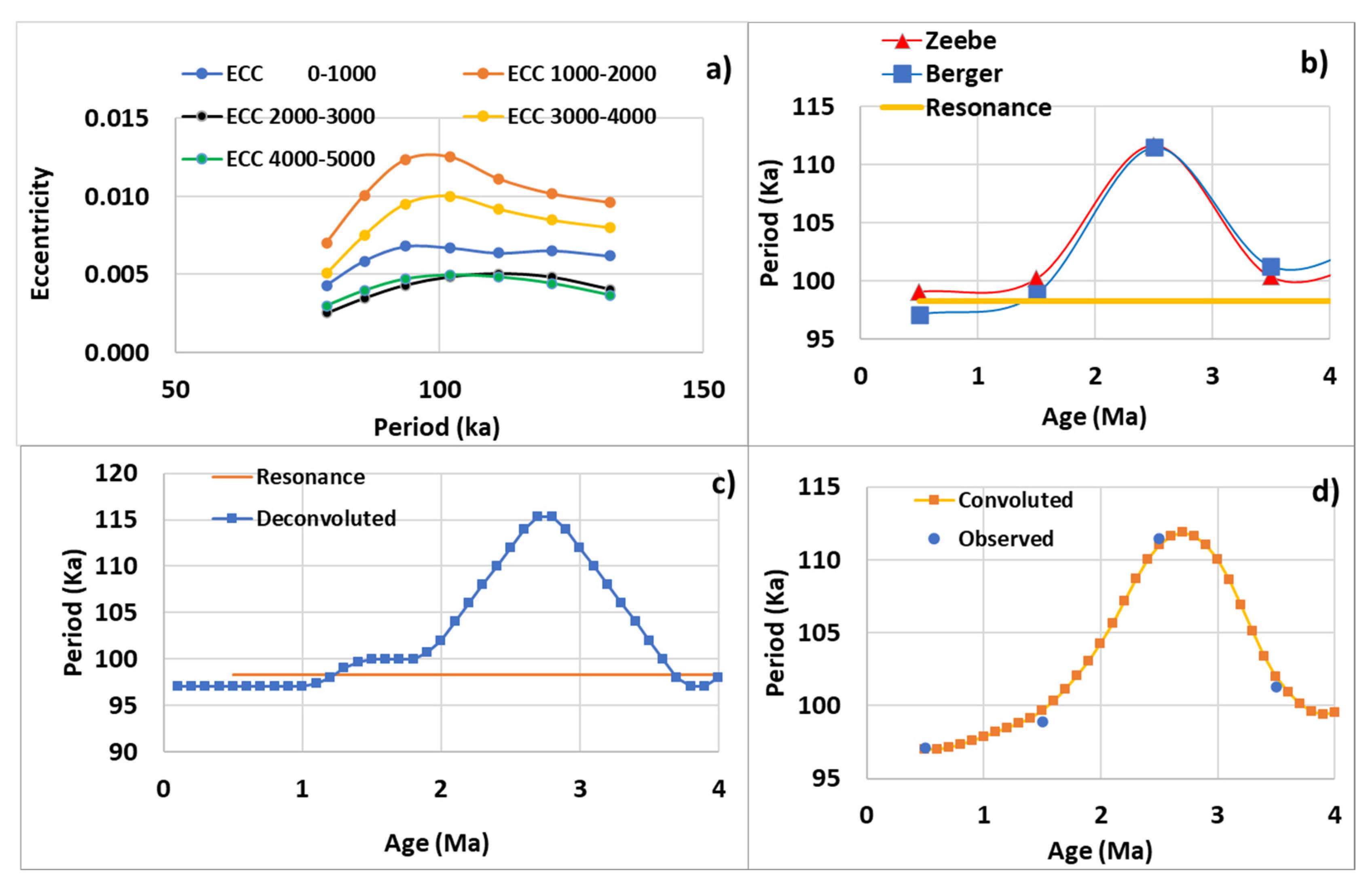
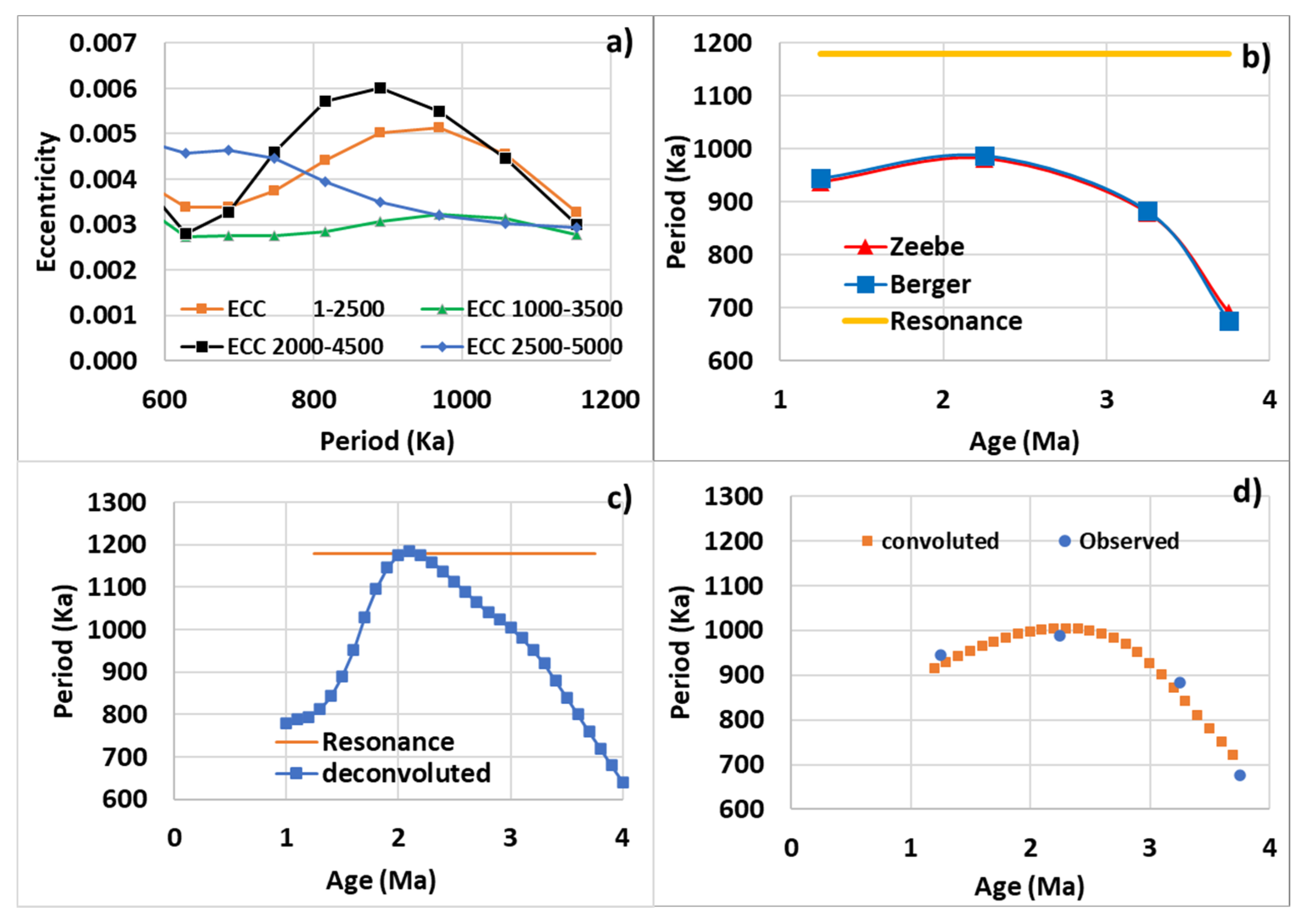
The poleward drift of the subtropical front of 4° during the MPT highlights an adjustment of the gyre to tune to the forcing period (~41 Ka) before the MPT while the subharmonic mode n 10 was dominant. After the MPT the subharmonic mode n 11 becomes dominant while its natural period approaches the forcing period (~100 Ka). An increase in the circumference of the gyre of almost 20% without displacement of the centroid allows the subharmonic mode n 11 to be tuned to the new forcing period while the natural period that characterizes the subharmonic mode n 10 is regained.
(2)
Thanks to the high resolution of the climate archive which spans 3.5 million years, the alkenone concentration at DSDP Site 593 presently situated north of the subtropical front allows to extend subharmonic modes beyond n 11 up to n 15 (Table 1). It is shown that modes n 13 and n 14 are subject to eccentricity forcing while modes n 12 and n 15 are pure subharmonics.
(3)
A transition of the dominant mode between two consecutive subharmonic modes occurs at the Pliocene-Pleistocene hinge. Like what happens during the MPT, the two subharmonic modes are forced simultaneously, and the natural period of the highest mode optimally tunes to the forcing period when both become very close.
(4)
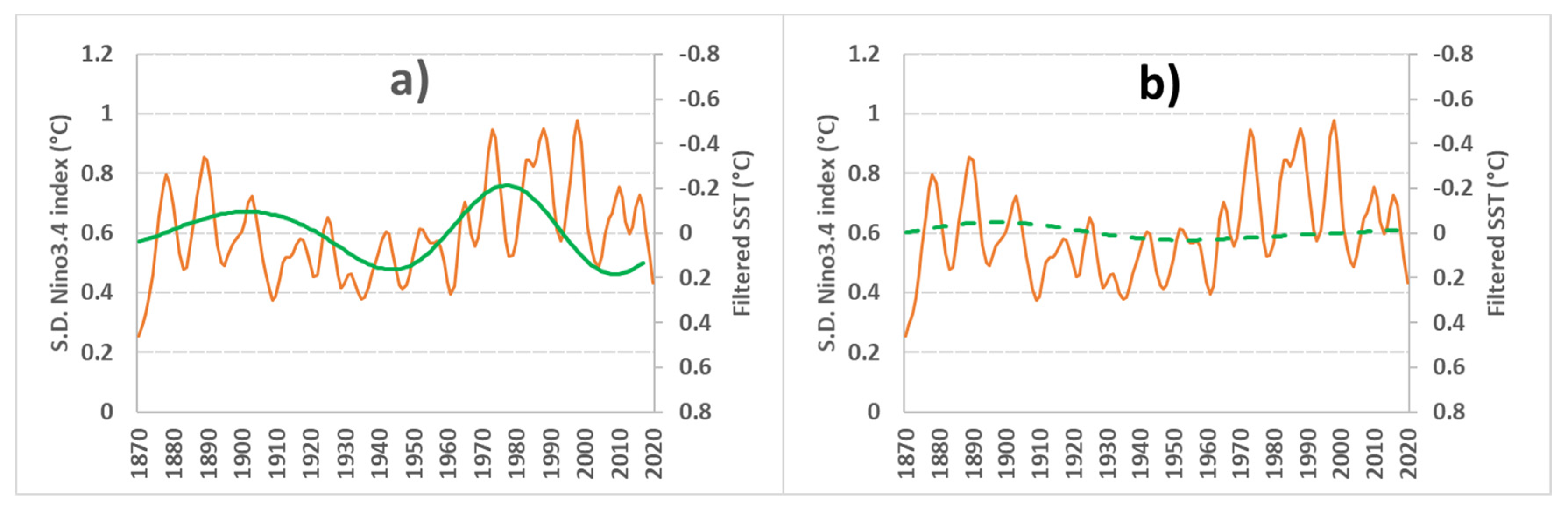
Variability of ENSO activity during the Holocene and the Last Glacial Maximum is subject to long-term adjustment of geostrophic forces in the equatorial Pacific. It is the amplitude of variation of the depth of the thermocline in the central and eastern Pacific which evolutes according to the subharmonic mode n 9 whose resonant period is 24.6 Ka, and not, as often stated, the frequency of events which occur on average every 4 years. This frequency is immutable, being intimately linked to the dynamics of the equatorial Pacific. Here again, the variability of ENSO during the Holocene and since 1870 is subject to the adjustment of geostrophic forces in the equatorial Pacific according to the subharmonic modes, n 6 in the first case (the resonant period is 3.1 Ka), and n 1 in the second (the resonant period is 64 years). Periods of warming induce a decrease in ENSO activity.
Unless it is contradicted by future research, the new approach based on the resonant forcing of long-period baroclinic waves in the oceans will probably take time to be largely accepted by the scientific community because of its novelty, which requires audacity. The notion of subharmonic modes indeed deeply changes understanding of the paleoclimate, including climate variations observed during the last two centuries [53,54].

Funding

This research received no external funding.

Acknowledgments

The author would particularly like to thank the patience and goodwill of the anonymous reviewers who agreed to evaluate this article which is intended to be very innovative, thus contributing to enriching a long work which has the audacity to think outside the box of paleoclimatology.

Conflicts of Interest

The author declares no conflict of interest.

References

  1. Hays, J.D.; Imbrie, J.; Shackleton, N.J. Variations in the Earth’s Orbit: Pacemaker of the Ice Ages. Science 1976, 194, 1121–1132. [Google Scholar] [CrossRef]
  2. Rial, J.; Anaclerio, C. Understanding nonlinear responses of the climate system to orbital forcing. Quat. Sci. Rev. 2000, 19, 1709–1722. [Google Scholar] [CrossRef]
  3. Hasselmann, K. Stochastic climate models Part I. Theory. Tellus 1976, 28, 473–485. [Google Scholar] [CrossRef] [Green Version]
  4. Benzi, R.; Parisi, G.; Sutera, A.; Vulpiani, A. Stochastic resonance in climatic change. Tellus 1982, 34, 10–15. [Google Scholar] [CrossRef]
  5. Nicolis, C. Stochastic aspects of climatic transitions—response to a periodic forcing. Tellus 1982, 34, 1–9. [Google Scholar] [CrossRef]
  6. Matteucci, G. A study of the climatic regimes of the Pleistocene using a stochastic resonance model. Clim. Dyn. 1991, 6, 67–81. [Google Scholar] [CrossRef]
  7. Nyman, K.H.M.; Ditlevsen, P.D. The middle Pleistocene transition by frequency locking and slow ramping of internal period. Clim. Dyn. 2019, 53, 3023–3038. [Google Scholar] [CrossRef] [Green Version]
  8. Ashwin, P.; Ditlevsen, P. The middle Pleistocene transition as a generic bifurcation on a slow manifold. Clim. Dyn. 2015, 45, 2683–2695. [Google Scholar] [CrossRef] [Green Version]
  9. Ditlevsen, P.D. Bifurcation structure and noise-assisted transitions in the Pleistocene glacial cycles. Paleoceanography 2009, 24. [Google Scholar] [CrossRef] [Green Version]
  10. Frankignoul, C.; Hasselmann, K. Stochastic climate models, Part II Application to sea-surface temperature anomalies and thermocline variability. Tellus 1977, 29, 289–305. [Google Scholar] [CrossRef] [Green Version]
  11. Saravanan, R.; McWilliams, J.C. Stochasticity and Spatial Resonance in Interdecadal Climate Fluctuations. J. Clim. 1997, 10, 2299–2320. [Google Scholar] [CrossRef]
  12. Sergin, V. Origin and Mechanism of Large-Scale Climatic Oscillations. Science 1980, 209, 1477–1482. [Google Scholar] [CrossRef] [PubMed]
  13. Ganopolski, A.; Rahmstorf, S. Abrupt Glacial Climate Changes due to Stochastic Resonance. Phys. Rev. Lett. 2002, 88, 038501. [Google Scholar] [CrossRef] [PubMed] [Green Version]
  14. Timmermann, A.; Gildor, H.; Schulz, M.; Tziperman, E. Coherent Resonant Millennial-Scale Climate Oscillations Triggered by Massive Meltwater Pulses. J. Clim. 2003, 16, 2569–2585. [Google Scholar] [CrossRef] [Green Version]
  15. Elderfield, H.; Ferretti, P.; Greaves, M.; Crowhurst, S.J.; McCave, I.N.; Hodell, D.A.; Piotrowski, A.M. Evolution of Ocean Temperature and Ice Volume Through the Mid-Pleistocene Climate Transition. Science 2012, 337, 704–709. [Google Scholar] [CrossRef]
  16. Mudelsee, M.; Schulz, M. The Mid-Pleistocene climate transition: Onset of 100 ka cycle lags ice volume build-up by 280 ka. Earth Planet. Sci. Lett. 1997, 151, 117–123. [Google Scholar] [CrossRef]
  17. Tziperman, E.; Gildor, H. On the mid-Pleistocene transition to 100-kyr glacial cycles and the asymmetry between glaciation and deglaciation times. Paleoceanography 2003, 18, 1. [Google Scholar] [CrossRef]
  18. Clark, P.U.; Archer, D.W.; Pollard, D.; Blum, J.D.; Rial, J.A.; Brovkin, V.; Mix, A.C.; Pisias, N.G.; Roy, M. The middle Pleistocene transition: Characteristics, mechanisms, and implications for long-term changes in atmospheric pCO2. Quat. Sci. Rev. 2006, 25, 3150–3184. [Google Scholar] [CrossRef] [Green Version]
  19. Chalk, T.B.; Hain, M.P.; Foster, G.L.; Rohling, E.J.; Sexton, P.F.; Badger, M.P.S.; Cherry, S.G.; Hasenfratz, A.P.; Haug, G.H.; Jaccard, S.L.; et al. Causes of ice age intensification across the Mid-Pleistocene Transition. Proc. Natl. Acad. Sci. USA 2017, 114, 13114–13119. [Google Scholar] [CrossRef] [Green Version]
  20. Hönisch, B.; Hemming, N.G.; Archer, D.; Siddall, M.; McManus, J.F. Atmospheric Carbon Dioxide Concentration across the Mid-Pleistocene Transition. Science 2009, 324, 1551–1554. [Google Scholar] [CrossRef]
  21. Quinn, C.; Sieber, J.; Von Der Heydt, A.S.; Lenton, T.M. The Mid-Pleistocene Transition induced by delayed feedback and bistability. Dyn. Stat. Clim. Syst. 2018, 3, 1–17. [Google Scholar] [CrossRef]
  22. Willeit, M.; Ganopolski, A.; Calov, R.; Brovkin, V. Mid-Pleistocene transition in glacial cycles explained by declining CO2and regolith removal. Sci. Adv. 2019, 5, eaav7337. [Google Scholar] [CrossRef] [PubMed] [Green Version]
  23. Lu, Z.; Liu, Z. Examining El Niño in the Holocene: Implications and challenges. Natl. Sci. Rev. 2018, 5, 807–809. [Google Scholar] [CrossRef]
  24. Tudhope, A.W.; Chilcott, C.P.; McCulloch, M.T.; Cook, E.R.; Chappell, J.; Ellam, R.M.; Lea, D.W.; Lough, J.M.; Shimmield, G.B. Variability in the El Nino-Southern Oscillation Through a Glacial-Interglacial Cycle. Science 2001, 291, 1511–1517. [Google Scholar] [CrossRef] [PubMed]
  25. McGregor, H.; Gagan, M.K. Western Pacific coral δ18O records of anomalous Holocene variability in the El Niño-Southern Oscillation. Geophys. Res. Lett. 2004, 31. [Google Scholar] [CrossRef] [Green Version]
  26. Cobb, K.M.; Charles, C.D.; Cheng, H.; Edwards, R.L. El Niño/Southern Oscillation and tropical Pacific climate during the last millennium. Nat. Cell Biol. 2003, 424, 271–276. [Google Scholar] [CrossRef]
  27. Cobb, K.M.; Westphal, N.; Sayani, H.R.; Watson, J.T.; Di Lorenzo, E.; Cheng, H.; Edwards, R.L.; Charles, C.D. Highly Variable El Niño–Southern Oscillation Throughout the Holocene. Science 2013, 339, 67–70. [Google Scholar] [CrossRef] [Green Version]
  28. Emile-Geay, J.; Cobb, K.M.; Carré, M.; Braconnot, P.; Leloup, J.; Zhou, Y.; Harrison, S.P.; Correge, T.; McGregor, H.V.; Collins, M.; et al. Links between tropical Pacific seasonal, interannual and orbital variability during the Holocene. Nat. Geosci. 2016, 9, 168–173. [Google Scholar] [CrossRef] [Green Version]
  29. Komugabe-Dixson, A.F.; Fallon, S.J.; Eggins, S.M.; Thresher, R.E. Radiocarbon evidence for mid-late Holocene changes in southwest Pacific Ocean circulation. Paleoceanography 2016, 31, 971–985. [Google Scholar] [CrossRef]
  30. Zhang, Z.; LeDuc, G.; Sachs, J.P. El Niño evolution during the Holocene revealed by a biomarker rain gauge in the Galápagos Islands. Earth Planet. Sci. Lett. 2014, 404, 420–434. [Google Scholar] [CrossRef] [Green Version]
  31. Grelaud, M.; Beaufort, L.; Cuven, S.; Buchet, N. Glacial to interglacial primary production and El Niño-Southern Oscillation dynamics inferred from coccolithophores of the Santa Barbara Basin. Paleoceanography 2009, 24, 1203. [Google Scholar] [CrossRef]
  32. Barr, C.; Tibby, J.; Leng, M.J.; Tyler, J.J.; Henderson, A.C.G.; Overpeck, J.T.; Simpson, G.L.; Cole, J.E.; Phipps, S.J.; Marshall, J.C.; et al. Holocene El Niño–Southern Oscillation variability reflected in subtropical Australian precipitation. Sci. Rep. 2019, 9, 1–9. [Google Scholar] [CrossRef] [PubMed]
  33. Koutavas, A.; Demenocal, P.B.; Olive, G.C.; Lynch-Stieglitz, J. Mid-Holocene El Niño–Southern Oscillation (ENSO) attenuation revealed by individual foraminifera in eastern tropical Pacific sediments. Geology 2006, 34, 993. [Google Scholar] [CrossRef]
  34. LeDuc, G.; Vidal, L.; Cartapanis, O.; Bard, E. Modes of eastern equatorial Pacific thermocline variability: Implications for ENSO dynamics over the last glacial period. Paleoceanography 2009, 24, 3202. [Google Scholar] [CrossRef]
  35. Koutavas, A.; Joanides, S. El Niño-Southern Oscillation extrema in the Holocene and Last Glacial Maximum. Paleoceanography 2012, 27, 4208. [Google Scholar] [CrossRef]
  36. Pinault, J.-L. Resonantly Forced Baroclinic Waves in the Oceans: Subharmonic Modes. J. Mar. Sci. Eng. 2018, 6, 78. [Google Scholar] [CrossRef] [Green Version]
  37. Explain with Realism Climate Variability. Available online: http://climatorealist.neowordpress.fr/ (accessed on 19 July 2020).
  38. Pinault, J.-L. Long Wave Resonance in Tropical Oceans and Implications on Climate: The Atlantic Ocean. Pure Appl. Geophys. 2013, 170, 1913–1930. [Google Scholar] [CrossRef]
  39. Pinault, J.-L. Long Wave Resonance in Tropical Oceans and Implications on Climate: The Pacific Ocean. Pure Appl. Geophys. 2015, 173, 2119–2145. [Google Scholar] [CrossRef]
  40. Pinault, J.-L. Resonance of baroclinic waves in the tropical oceans: The Indian Ocean and the far western Pacific. Dyn. Atmos. Oceans 2020, 89, 101119. [Google Scholar] [CrossRef]
  41. Torrence, C.; Compo, G.P. A practical guide for wavelet analysis. Bull. Am. Meteorol. Soc. 1998, 79, 61–78. [Google Scholar] [CrossRef] [Green Version]
  42. Pinault, J.-L. Anticipation of ENSO: What teach us the resonantly forced baroclinic waves. Geophys. Astrophys. Fluid Dyn. 2016, 110, 518–528. [Google Scholar] [CrossRef]
  43. Pinault, J.-L. The Anticipation of the ENSO: What Resonantly Forced Baroclinic Waves Can Teach Us (Part II). J. Mar. Sci. Eng. 2018, 6, 63. [Google Scholar] [CrossRef] [Green Version]
  44. Pinault, J.-L. Modulated Response of Subtropical Gyres: Positive Feedback Loop, Subharmonic Modes, Resonant Solar and Orbital Forcing. J. Mar. Sci. Eng. 2018, 6, 107. [Google Scholar] [CrossRef] [Green Version]
  45. Pinault, J.-L. Resonant Forcing of the Climate System in Subharmonic Modes. J. Mar. Sci. Eng. 2020, 8, 60. [Google Scholar] [CrossRef] [Green Version]
  46. McClymont, E.L.; Elmore, A.C.; Kender, S.; Leng, M.J.; Greaves, M.; Elderfield, H. Pliocene-Pleistocene evolution of sea surface and intermediate water temperatures from the southwest Pacific. Paleoceanography 2016, 31, 895–913. [Google Scholar] [CrossRef] [PubMed] [Green Version]
  47. Ballegeer, A.-M.; Flores, J.A.; Sierro, F.J.; Andersen, N. Monitoring fluctuations of the Subtropical Front in the Tasman Sea between 3.45 and 2.45Ma (ODP site 1172). Palaeogeogr. Palaeoclim. Palaeoecol. 2012, 313–314, 215–224. [Google Scholar] [CrossRef]
  48. Berger, A.; Loutre, M.-F. Insolation values for the climate of the last 10 million years. Quat. Sci. Rev. 1991, 10, 297–317. [Google Scholar] [CrossRef]
  49. Zeebe, R.E.; Lourens, L. Solar System chaos and the Paleocene–Eocene boundary age constrained by geology and astronomy. Science 2019, 365, 926–929. [Google Scholar] [CrossRef] [Green Version]
  50. Grootes, P.M.; Stuiver, M. Oxygen 18/16 variability in Greenland snow and ice with 10−3- to 105-year time resolution. J. Geophys. Res. Space Phys. 1997, 102, 26455–26470. [Google Scholar] [CrossRef]
  51. Jouzel, J.; Masson-Delmotte, V.; Cattani, O.; Dreyfus, G.; Falourd, S.; Hoffmann, G.; Minster, B.; Nouet, J.; Barnola, J.-M.; Chappellaz, J.; et al. Orbital and Millennial Antarctic Climate Variability over the Past 800,000 Years. Science 2007, 317, 793–796. [Google Scholar] [CrossRef] [Green Version]
  52. Rayner, N.A.; Parker, D.E.; Horton, E.B.; Folland, C.K.; Alexander, L.V.; Rowell, D.P.; Kent, E.C.; Kaplan, A.L. Global analyses of sea surface temperature, sea ice, and night marine air temperature since the late nineteenth century. J. Geophys. Res. Space Phys. 2003, 108, 4407. [Google Scholar] [CrossRef]
  53. Pinault, J.-L. Anthropogenic and Natural Radiative Forcing: Positive Feedbacks. J. Mar. Sci. Eng. 2018, 6, 146. [Google Scholar] [CrossRef] [Green Version]
  54. Pinault, J.-L. The Moist Adiabat, Key of the Climate Response to Anthropogenic Forcing. Climate 2020, 8, 45. [Google Scholar] [CrossRef] [Green Version]
Figure 1. Location of boreholes Deep Sea Drilling Project (DSDP) 593 (in green) and ODP 1172 (in red) in the Tasman Sea.
Jmse 09 00013 g001
Figure 2. Location of the borehole V21–30 (in red) in the eastern equatorial Pacific near the Galapagos Islands.
Jmse 09 00013 g002
Figure 3. Variations in the period of eccentricity in the vicinity of 100 Ka calculated from Berger and Loutre [47]—(a) Fourier transform of eccentricity variations over 1 Ma time intervals—(b) Periods vs. time observed at the maximums of the Fourier transforms in a). The same values calculated from Zeebe and Lourens [49] are also represented—(c) Deconvoluted curve of the period vs. time represented in (bd) Comparison of the moving average over 1 Ma of the deconvoluted curve in (c) and the period vs. time in (b).
Jmse 09 00013 g003
Figure 4. Data used in the present study—(a) Alkenone concentration vs. time at DSDP Site 593 used as a proxy of Sea Surface Temperatures (SST)—(b) Fourier transform (FT) of SST vs. time. Maximums of the peaks are in Ka—(c) FT of Total Solar Irradiance (TSI)—(d) FT of eccentricity variations—(e) Coherence of TSI and SST vs. period—(f) Coherence of TSI and SST vs. time.
Jmse 09 00013 g004
Figure 5. Orbital forcing and SST response into the band 295–590 Ka—(a) Total solar irradiance (TSI)—(b) Forcing efficiency—(c) Comparison of the TSI multiplied by the forcing efficiency from (b) in red and the SST in blue—(df) same as (ac) transposed to the band 590–1769 Ka.
Jmse 09 00013 g005
Figure 6. Orbital forcing and responses of SST and sea water temperature (T) into the band 1769–3500 Ka—(a) Total Solar Irradiance (TSI)—(b) SST de-trended and filtered—(c) Benthic foraminiferal Mg/Ca analysis vs. time at DSDP Site 593 used as a proxy of T—(d) T de-trended and filtered.
Jmse 09 00013 g006
Figure 7. Variations in the period of eccentricity in the vicinity of 1000 Ka calculated from Berger and Loutre [47]—(a) Fourier transform of eccentricity variations over 2.5 Ma time intervals—(b) Periods vs. time observed at the maximums of the Fourier transforms in (a). The same values calculated from Zeebe and Lourens [49] are also represented—(c) Deconvoluted curve of the period vs. time represented in (bd) Comparison of the moving average over 2.5 Ma of the deconvoluted curve in (c) and the period vs. time in (b).
Jmse 09 00013 g007
Figure 8. Variations in the δ O   18 standard deviation of individual G. ruber from the Holocene and Last Glacial Maximum. The high bar in red of snapshots represents the square root of the total variance of δ O   18 obtained from all the data while the low bar in blue excludes the heaviest and lightest value from each distribution. The bar on left indicates the 1958–2007 monthly δ O   18 standard deviation from instrumental SST and salinity. Values marked with an asterisk are recognized as doubtful by the author [35]—(a) Obtained from Greenland Ice Sheet Project 2 (GISP2) δ O   18 record filtered in the 18.4—36.9 Ka band, a proxy of long-term adjustment of geostrophic forces is drawn in green (the record is converted into the global temperature T through the calibration T = 1.42 × δ O   18 + 49.0 )—(b) GISP2 δ O   18 record is filtered in the 2.3–4.6 Ka band.
Jmse 09 00013 g008
Figure 9. Standard deviation of the Nino3.4 index in the 1.5–7 years band (in red) and estimation of the filtered global temperature from the linear combination of SST anomalies 0.75 × N A + 0.25 × N P located [36° N, 39° N] × [30° W, 40° W] in the North Atlantic (NA), and [30° N, 33° N] × [170° E, 180° E] in the North Pacific (NP) subtropical gyres (in green)—(a) SST anomalies filtered in the 48–96 years band—(b) SST anomalies filtered in the 96–150 years band.
Jmse 09 00013 g009
Table 1. The natural periods of Gyral Rossby Waves (GRWs), and the bands characteristic of subharmonic modes. Each subharmonic mode is built by recurrence from the observations as indicated in the introduction. Previous modes were defined in [45].
RankBand Width (yr)Period of Resonance (yr)Subharmonic Mode Forcing Mode
12147,456–294,912196,608 n 12 = 3 × 2 10 No external forcing
13294,912–589,824393,216 n 13 = 3 × 2 11 Orbital forcing (eccentricity)
14589,824–1,769,4721,179,648 n 14 = 3 2 × 2 11 Orbital forcing (eccentricity)
151,769,472–3,538,9442,359,296 n 15 = 3 2 × 2 12 No external forcing
Publisher’s Note: MDPI stays neutral with regard to jurisdictional claims in published maps and institutional affiliations.

