A Modeling Comparison of the Potential Effects on Marine Mammals from Sounds Produced by Marine Vibroseis and Air Gun Seismic Sources

 ,
,
Abstract
1. Introduction
2. Methods
2.1. Scenarios
2.2. Comparison
2.3. Computation
2.3.1. Sources Levels
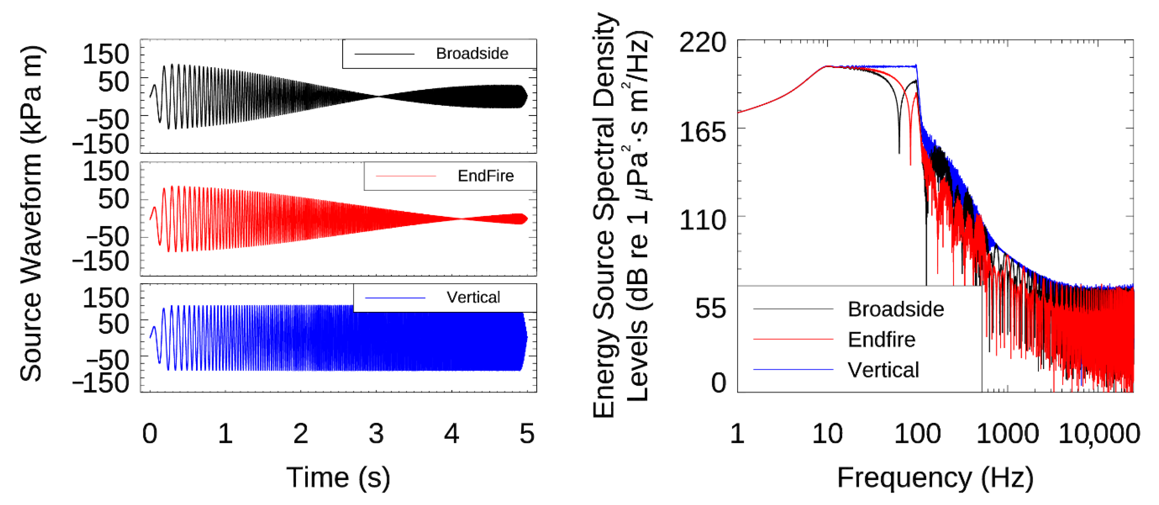
Marine Vibroseis (MV)
Air Gun Arrays
2.3.2. Sound Propagation
Sound Propagation Models
Environmental Parameters
Ambient Sound Levels
2.3.3. Surveys Characteristics
2.3.4. Received Signal Characteristics
2.3.5. Agent-Based Model
3. Results
3.1. Signal Characteristics with Distance
3.2. Exposure Estimates from Agent-Based Model
4. Discussion
5. Conclusions
Author Contributions
Funding
Acknowledgments
Conflicts of Interest
References
- Parkes, G.E.; Hatton, L. The Marine Seismic Source, 1st ed.; Springer Science & Business Media: Dordrecht, The Netherlands, 1986. [Google Scholar]
- Carroll, P. A note on synthetic vibroseis sweep generation. Can. J. Explor. Geophys. 1971, 7, 80–82. [Google Scholar]
- International Organization for Standardization. Underwater Acoustics—Terminology; ISO 18405:2017; ISO: Geneva, Switzerland, 2017; p. 51. [Google Scholar]
- Spence, J.H. Seismic survey noise under examination. In Offshore: World Trends and Technology for Offshore Oil and Gas Operations; Endeavor Business Media LCC.: Nashville, TN, USA, 2009; Volume 69. [Google Scholar]
- LGL. Environmental Assessment of Marine Vibroseis; Report for the Joint Industry Programme on E&P Sound and Marine Life; LGL: King City, CA, USA; Marine Acoustics Inc.: Middletown, RI, USA, 2011; p. 207. [Google Scholar]
- Green, D.M.; Swets, J.A. Signal Detection Theory and Psychophysics; Krieger: Huntington, WV, USA, 1974. [Google Scholar]
- Moore, B.C.J. An Introduction to the Psychology of Hearing, 6th ed.; Emerald Group Publishing: Bingley, UK, 2012. [Google Scholar]
- Erbe, C.; Reichmuth, C.; Cunningham, K.; Lucke, K.; Dooling, R. Communication Masking in Marine Mammals: A Review and Research Strategy. Mar. Pollut. Bull. 2016, 103, 15–38. [Google Scholar] [CrossRef]
- Southall, B.L.; Bowles, A.E.; Ellison, W.T.; Finneran, J.J.; Gentry, R.L.; Greene, C.R., Jr.; Kastak, D.; Ketten, D.R.; Miller, J.H.; Nachtigall, P.E.; et al. Marine Mammal Noise Exposure Criteria: Initial Scientific Recommendations. Aquat. Mamm. 2007, 33, 411–521. [Google Scholar] [CrossRef]
- Martin, S.B.; Lucke, K.; Barclay, D.R. Techniques for Distinguishing between Impulsive and Non-Impulsive Sound in the Context of Regulating Sound Exposure for Marine Mammals. J. Acoust. Soc. Am. 2020, 147, 2159–2176. [Google Scholar] [CrossRef]
- Popper, A.N.; Hawkins, A.D.; Fay, R.R.; Mann, D.A.; Bartol, S.; Carlson, T.J.; Coombs, S.; Ellison, W.T.; Gentry, R.L.; Halvorsen, M.B.; et al. Sound Exposure Guidelines for Fishes and Sea Turtles: A Technical Report Prepared by ANSI-Accredited Standards Committee S3/SC1 and Registered with ANSI; ASA S3/SC1.4 TR-2014; ASA Press: Washington, DC, USA; Springer: Berlin/Heidelberg, Germany, 2014. [Google Scholar]
- Southall, B.L.; Finneran, J.J.; Reichmuth, C.J.; Nachtigall, P.E.; Ketten, D.R.; Bowles, A.E.; Ellison, W.T.; Nowacek, D.P.; Tyack, P.L. Marine Mammal Noise Exposure Criteria: Updated Scientific Recommendations for Residual Hearing Effects. Aquat. Mamm. 2019, 45, 125–232. [Google Scholar] [CrossRef]
- National Marine Fisheries Service. 2018 Revision to: Technical Guidance for Assessing the Effects of Anthropogenic Sound on Marine Mammal Hearing (Version 2.0): Underwater Thresholds for Onset of Permanent and Temporary Threshold Shifts; US Department of Commerce: Washington, DC, USA; NOAA: Washington, DC, USA, 2018; p. 167. [Google Scholar]
- Ellison, W.T.; Frankel, A.S. A common sense approach to source metrics. In The Effects of Noise on Aquatic Life; Popper, A.N., Hawkins, A.D., Eds.; Springer: New York, NY, USA, 2012; pp. 433–438. [Google Scholar]
- National Oceanic and Atmospheric Administration. Notice of Public Scoping and Intent to Prepare an Environmental Impact Statement; NOAA: Washington, DC, USA, 2005. [Google Scholar]
- Malme, C.I.; Miles, P.R.; Clark, C.W.; Tyack, P.L.; Bird, J.E. Investigations of the Potential Effects of Underwater Noise from Petroleum Industry Activities on Migrating Gray Whale Behavior. Phase II: January 1984 migration; US Department of the Interior. Minerals Management Service: Cambridge, MA, USA, 1984. [Google Scholar]
- Richardson, W.J.; Würsig, B.; Greene, C.R., Jr. Reactions of bowhead whales, Balaena mysticetus, to drilling and dredging noise in the Canadian Beaufort Sea. Mar. Environ. Res. 1990, 29, 135–160. [Google Scholar] [CrossRef]
- Richardson, W.J.; Würsig, B.; Greene, C.R., Jr. Reactions of bowhead whales, Balaena mysticetus, to seismic exploration in the Canadian Beaufort Sea. J. Acoust. Soc. Am. 1986, 79, 1117–1128. [Google Scholar] [CrossRef]
- Malme, C.I.; Miles, P.R.; Clark, C.W.; Tyack, P.L.; Bird, J.E. Investigations of the Potential Effects of Underwater Noise from Petroleum Industry Activities on Migrating Gray Whale Behavior; US Department of the Interior: Washington, DC, USA; Minerals Management Service: Cambridge, MA, USA, 1983. [Google Scholar]
- Nedwell, J.R.; Turnpenny, A.W.; Lovell, J.; Parvin, S.J.; Workman, R.; Spinks, J.A.L.; Howell, D. A Validation of the dBht as a Measure of the Behavioural and Auditory Effects of Underwater Noise; Department for Business, Enterprise and Regulatory Reform: London, UK, 2007; p. 74. [Google Scholar]
- Wood, J.D.; Southall, B.L.; Tollit, D.J. PG&E offshore 3-D Seismic Survey Project Environmental Impact Report–Marine Mammal Technical Draft Report; SMRU Ltd.: St Andrews, UK, 2012; p. 121. [Google Scholar]
- Department of the Navy (US). Final Supplemental Environmental Impact Statement/Supplemental Overseas Environmental Impact Statement for Surveillance Towed Array Sensor System Low Frequency Active (SURTASS LFA) Sonar; Department of the Navy: Washington, DC, USA, 2012. [Google Scholar]
- Feller, W. An Introduction to Probability Theory and Its Applications, 3rd ed.; John Wiley & Sons: New York, NY, USA, 1968; Volume 1. [Google Scholar]
- McConnell, J.A.; Berkman, E.F.; Murray, B.S.; Abraham, B.M. Coherent Sound Source for Marine Seismic Surveys. U.S. Patent 9,625,598, 18 April 2017. [Google Scholar]
- McConnell, J.A.; Berkman, E.F.; Murray, B.S.; Abraham, B.M.; Roy, D.A. Coherent Sound Source for Marine Seismic Surveys. U.S. Patent 9,562,982, 18 April 2017. [Google Scholar]
- Tellier, N.; Ollivrin, G. Low-frequency Vibroseis: Current achievements and the road ahead? First Break 2019, 37, 49–54. [Google Scholar] [CrossRef]
- Sallas, J.; Gibson, J.; Maxwell, P.; Lin, F. Pseudorandom sweeps for simultaneous sourcing and low-frequency generation. Lead. Edge 2011, 30, 1162–1172. [Google Scholar] [CrossRef]
- Scholtz, P. Pseudo-random sweeps for built-up area seismic surveys. Lead. Edge 2013, 32, 276–282. [Google Scholar] [CrossRef]
- Dean, T. Establishing the limits of vibrator performance-experiments with pseudorandom sweeps. In SEG Technical Program Expanded Abstracts 2012; Society of Exploration Geophysicists: Tulsa, OK, USA, 2012; pp. 1–5. [Google Scholar]
- Dean, T. The use of pseudorandom sweeps for vibroseis surveys. Geophys. Prospect. 2014, 62, 50–74. [Google Scholar] [CrossRef]
- Dean, T.; Tulett, J.; Lane, D. The use of pseudorandom sweeps for vibroseis acquisition. First Break 2017, 35, 107–112. [Google Scholar]
- Feltham, A.; Girard, M.; Jenkerson, M.; Nechayuk, V.; Griswold, S.; Henderson, N.; Johnson, G. The Marine Vibrator Joint Industry Project: Four years on. Explor. Geophys. 2017, 49, 675–687. [Google Scholar] [CrossRef]
- Schostak, B.; Jenkerson, M. The Marine Vibrator Joint Industry Project. In SEG Technical Program Expanded Abstracts; Society of Exploration Geophysicists: Tulsa, OK, USA, 2015; pp. 4961–4962. [Google Scholar]
- Ainslie, M.A. Principles of Sonar Performance Modeling; Praxis Books; Springer: Berlin/Heidelberg, Germany, 2010. [Google Scholar]
- Ainslie, M.A.; de Jong, C.A.F.; Martin, S.B.; Miksis-Olds, J.L.; Warren, J.D.; Heaney, K.D.; Hillis, C.A.; MacGillivray, A.O. ADEON Project Dictionary: Terminology Standard; JASCO: Oklahoma City, OK, USA, 2020. [Google Scholar]
- Sallas, J.; Teyssandier, B. Vibrator Source Array Load-Balancing Method and System. U.S. Patent 9482765, 1 November 2016. [Google Scholar]
- Teyssandier, B.; Sallas, J.J. The shape of things to come—Development and testing of a new marine vibrator source. Lead. Edge 2019, 38, 680–690. [Google Scholar] [CrossRef]
- Scandrett, C.L.; Baker, S.R. Pritchard’s Approximation in Array Modeling; Naval Postgraduate School: Monterey, CA, USA, 1999. [Google Scholar]
- MacGillivray, A.O. An Acoustic Modelling Study of Seismic Airgun Noise in Queen Charlotte Basin; University of Victoria: Victoria, BC, Canada, 2006; p. 98. [Google Scholar]
- Ziolkowski, A.M. A method for calculating the output pressure waveform from an air gun. Geophys. J. Int. 1970, 21, 137–161. [Google Scholar] [CrossRef]
- Dragoset, W.H. A comprehensive method for evaluating the design of airguns and airgun arrays. In Proceedings of the 16th Annual Offshore Technology Conference, Houston, TX, USA, 7–9 May 1984; pp. 75–84. [Google Scholar]
- Laws, R.M.; Hatton, L.; Haartsen, M. Computer modeling of clustered airguns. First Break 1990, 8, 331–338. [Google Scholar] [CrossRef]
- Landro, M. Modeling of GI gun signatures. Geophys. Prospect. 1992, 40, 721–747. [Google Scholar] [CrossRef]
- Mattsson, A.; Jenkerson, M. Single Airgun and Cluster Measurement Project. In Joint Industry Programme (JIP) on Exploration and Production Sound and Marine Life Proramme Review; International Association of Oil and Gas Producers: Houston, TX, USA, 2008. [Google Scholar]
- Zhang, Z.Y.; Tindle, C.T. Improved equivalent fluid approximations for a low shear speed ocean bottom. J. Acoust. Soc. Am. 1995, 98, 3391–3396. [Google Scholar] [CrossRef]
- Collins, M.D.; Cederberg, R.J.; King, D.B.; Chin-Bing, S. Comparison of algorithms for solving parabolic wave equations. J. Acoust. Soc. Am. 1996, 100, 178–182. [Google Scholar] [CrossRef]
- Collins, M.D. A split-step Padé solution for the parabolic equation method. J. Acoust. Soc. Am. 1993, 93, 1736–1742. [Google Scholar] [CrossRef]
- Hannay, D.E.; Racca, R.G. Acoustic Model Validation; JASCO Research Ltd.: Oklahoma City, OK, USA, 2005; p. 34. [Google Scholar]
- Porter, M.B.; Liu, Y.C. Finite-element ray tracing. In Proceedings of the International Conference on Theoretical and Computational, Manchester, UK, 13–16 December 1994; pp. 947–956. [Google Scholar]
- MacGillivray, A.O.; Chapman, N.R. Modeling underwater sound propagation from an airgun array using the parabolic equation method. Can. Acoust. 2012, 40, 19–25. [Google Scholar] [CrossRef][Green Version]
- Aerts, L.A.M.; Blees, M.; Blackwell, S.B.; Greene, C.R., Jr.; Kim, K.H.; Hannay, D.E.; Austin, M.E. Marine Mammal Monitoring and Mitigation during BP Liberty OBC Seismic Survey in Foggy Island Bay, Beaufort Sea, July-August 2008: 90-Day Report; NOAA: Washington, DC, USA, 2008; p. 199. [Google Scholar]
- Funk, D.W.; Hannay, D.E.; Ireland, D.S.; Rodrigues, R.; Koski, W.R. Marine Mammal Monitoring and Mitigation during Open Water Seismic Exploration by Shell Offshore Inc. in the Chukchi and Beaufort Seas, July–November 2007: 90-Day Report; NOAA: Washington, DC, USA, 2008; p. 218. [Google Scholar]
- Funk, D.W.; Hannay, D.E.; Ireland, D.S.; Rodrigues, R.; Koski, W.R. Marine Mammal Monitoring and Mitigation during Open Water Seismic Exploration by Shell Offshore Inc. in the Chukchi and Beaufort Seas, July–October 2008: 90-Day Report; NOAA: Washington, DC, USA, 2009; p. 277. [Google Scholar]
- O’Neill, C.; Leary, D.; McCrodan, A. Sound Source Verification. In Marine Mammal Monitoring and Mitigation during open water seismic exploration by Statoil USA E&P Inc. in the Chukchi Sea, August-October 2010: 90-Day Report; Blees, M.K., Ed.; LGL Report P1119; NOAA: Washington, DC, USA, 2010; pp. 1–34. [Google Scholar]
- Warner, G.A.; Erbe, C.; Hannay, D.E. Underwater Sound Measurements. In Marine Mammal Monitoring and Mitigation during Open Water Shallow Hazards and Site Clearance Surveys by Shell Offshore Inc. in the Alaskan Chukchi Sea, July-October 2009: 90-Day Report; Reiser, C.M., Ed.; NOAA: Washington, DC, USA, 2010; pp. 1–54. [Google Scholar]
- Racca, R.G.; Rutenko, A.N.; Bröker, K.; Gailey, G. Model Based Sound Level Estimation and in-Field Adjustment for Real-Time Mitigation of Behavioural Impacts from a Seismic Survey and Post-Event Evaluation of Sound Exposure for Individual Whales; Acoustics: Fremantle, Australia, 2012. [Google Scholar]
- Racca, R.G.; Rutenko, A.N.; Bröker, K.; Austin, M.E. A Line in the Water—Design and Enactment of a Closed Loop, Model Based Sound Level Boundary Estimation Strategy for Mitigation of Behavioural Impacts from a Seismic Survey. In Proceedings of the 11th European Conference on Underwater Acoustics, Edinburgh, UK, 2–6 July 2012. [Google Scholar]
- Martin, B.; Bröker, K.; Matthews, M.-N.R.; MacDonnell, J.T.; Bailey, L. Comparison of measured and modeled air-gun array sound levels in Baffin Bay, West Greenland. In Proceedings of the OceanNoise, Barcelona, Spain, 11–15 May 2015. [Google Scholar]
- Hamilton, E.L. Geoacoustic modeling of the sea floor. J. Acoust. Soc. Am. 1980, 68, 1313–1340. [Google Scholar] [CrossRef]
- Buckingham, M.J. Compressional and Shear Wave Properties of Marine Sediments: Comparisons between Theory and data. J. Acoust. Soc. Am. 2005, 117, 137–152. [Google Scholar] [CrossRef] [PubMed]
- Hanebuth, T.J.J.; Voris, H.K.; Yokoyama, Y.; Saito, Y.; Okuno, J. Formation and fate of sedimentary depocentres on Southeast Asia’s Sunda Shelf over the past sea-level cycle and biogeographic implications. Earth-Sci. Rev. 2011, 104, 92–110. [Google Scholar] [CrossRef]
- Bishop, M.G. Petroleum Systems of the Northwest Java Province, Java and offshore Southeast Sumatra, Indonesia, in Open-File Report; US Department of the Interior: Washington, DC, USA; US Geological Survey: Reston, VA, USA, 2000; p. 31. [Google Scholar]
- [NPD] Oljedirektoratet–Norwegian Petroleum Directorate. The NPD’s Fact-pages-Hordaland Group. 2011. Available online: http://www.npd.no/engelsk/cwi/pbl/en/su/all/67.htm (accessed on 21 December 2020).
- Shipboard Scientific Party. Site 96, Leg 619. In Deep Sea Drilling Projects Initial Reports; US Government Printing Office: Washington, DC, USA, 1987. [Google Scholar]
- Teague, W.J.; Carron, M.J.; Hogan, P.J. A comparison between the Generalized Digital Environmental Model and Levitus climatologies. J. Geophys. Res. 1990, 95, 7167–7183. [Google Scholar] [CrossRef]
- Carnes, M.R. Description and Evaluation of GDEM-V 3.0; MS. NRL Memorandum Report 7330-09-9165; US Naval Research Laboratory, Stennis Space Center: New Orleans, MS, USA, 2009; p. 21. [Google Scholar]
- Coppens, A.B. Simple equations for the speed of sound in Neptunian waters. J. Acoust. Soc. Am. 1981, 69, 862–863. [Google Scholar] [CrossRef]
- Mahanty, M.M.; Sanjana, M.C.; Latha, G.; Raguraman, G. An Investigation on the Fluctuation and Variability of Ambient Noise in Shallow Waters of South West Bay of Bengal; National Institute of Science Communication and Information Resources: New Delhi, India, 2014; Volume 43, pp. 747–753. [Google Scholar]
- International Electrotechnical Commission. IEC 61260-1:2014 Electroacoustics—Octave-Band and Fractional-Octave-Band Filters—Part 1: Specifications; IEC: London, UK, 2014; p. 88. [Google Scholar]
- Merchant, N.D.; Brookes, K.L.; Faulkner, R.C.; Bicknell, A.W.J.; Godley, B.J.; Witt, M.J. Underwater noise levels in UK waters. Sci. Rep. 2016, 6, 1–10. [Google Scholar] [CrossRef]
- Wiggins, S.M.; Hall, J.M.; Thayre, B.J.; Hildebrand, J.A. Gulf of Mexico low-frequency ocean soundscape impacted by airguns. J. Acoust. Soc. Am. 2016, 140, 176–183. [Google Scholar] [CrossRef]
- Urick, R.J. Principles of Underwater Sound, 3rd ed.; McGraw-Hill: New York, NY, USA; London, UK, 1983; p. 423. [Google Scholar]
- Martin, B.; MacDonnell, J.T.; Bröker, K. Cumulative sound exposure levels—Insights from seismic survey measurements. J. Acoust. Soc. Am. 2017, 141, 3603. [Google Scholar] [CrossRef]
- Plomp, R.; Bouman, M.A. Relation between Hearing Threshold and Duration for Tone Pulses. J. Acoust. Soc. Am. 1959, 31, 749–758. [Google Scholar] [CrossRef]
- MacGillivray, A.O.; Racca, R.G.; Li, Z. Marine mammal audibility of selected shallow-water survey sources. J. Acoust. Soc. Am. 2014, 135, EL35–EL40. [Google Scholar] [CrossRef] [PubMed]
- Houser, D.S. A method for modeling marine mammal movement and behavior for environmental impact assessment. IEEE J. Ocean. Eng. 2006, 31, 76–81. [Google Scholar] [CrossRef]
- Ellison, W.T.; Clark, C.W.; Bishop, G.C. Potential use of surface reverberation by bowhead whales, Balaena mysticetus, in under-ice navigation: Preliminary considerations. In Report of the International Whaling Commission; International Whaling Commission: Cambridge, UK, 1987; pp. 329–332. [Google Scholar]
- Frankel, A.S.; Ellison, W.T.; Buchanan, J. Application of the acoustic integration model (AIM) to predict and minimize environmental impacts. In OCEANS’02 MTS/IEEE; IEEE: Biloxi, MI, USA, 2002; pp. 1438–1443. [Google Scholar]
- Kaschner, K.; Rius-Barile, J.; Kesner-Reyes, K.; Garilao, C.; Kullander, S.O.; Rees, T.; Froese, R. AquaMaps: Predicted Range Maps for Aquatic Species; World Wide Web Electronic Publication. 2016. Available online: www.aquamaps.org (accessed on 21 December 2020).
- Kreb, D. Cetacean diversity and habitat preferences in tropical waters of East Kalimantan, Indonesia. Raffles Bull. Zool. 2005, 53, 149–155. [Google Scholar]
- Shirakihara, K.; Shirakihara, M.; Yamamoto, Y. Distribution and abundance of finless porpoise in the Inland Sea of Japan. Mar. Biol. 2007, 150, 1025–1032. [Google Scholar] [CrossRef]
- Reyne, M.; Webster, I.; Huggins, A. A Preliminary Study on the Sea Turtle Density in Mauritius. Mar. Turt. Newsl. 2017, 152, 5–8. [Google Scholar]
- Hammond, P.S.; Macleod, K.; Berggren, P.; Borchers, D.L.; Burt, L.; Cañadas, A.; Desportes, G.; Donovan, G.P.; Gilles, A.; Gillespie, D. Cetacean abundance and distribution in European Atlantic shelf waters to inform conservation and management. Biol. Conserv. 2013, 164, 107–122. [Google Scholar] [CrossRef]
- [DoN] Department of the Navy (US). Navy OPAREA Density Estimate (NODE) for the Gulf of Mexico; Contract #N62470-02 D-9997, CTO 0030; Department of the Navy: Washington, DC, USA, 2007. [Google Scholar]
- Roberts, J.J.; Best, B.D.; Mannocci, L.; Fujioka, E.; Halpin, P.N.; Palka, D.L.; Garrison, L.P.; Mullin, K.D.; Cole, T.V.N.; Khan, C.B.; et al. Habitat-based cetacean density models for the U.S. Atlantic and Gulf of Mexico. Sci. Rep. 2016, 6, 22615. [Google Scholar] [CrossRef]
- [NOAA] National Oceanic and Atmospheric Administration (US). Notice of Public Scoping and Intent to Prepare an Environmental Impact Statement. Fed. Regist. 2005, 70, 1871–1875. [Google Scholar]
- Richardson, W.J.; Greene, C.R., Jr.; Malme, C.I.; Thomson, D.H. Marine Mammals and Noise; Academic Press: San Diego, CA, USA, 1995; p. 576. [Google Scholar]
- Gordon, J.; Gillespie, D.; Potter, J.R.; Frantzis, A.; Simmonds, M.P.; Swift, R.; Thompson, D. A Review of the Effects of Seismic Surveys on Marine Mammals. Mar. Technol. Soc. J. 2003, 37, 16–34. [Google Scholar] [CrossRef]
- Nowacek, D.P.; Thorne, L.H.; Johnston, D.W.; Tyack, P.L. Responses of cetaceans to anthropogenic noise. Mammal Rev. 2007, 37, 81–115. [Google Scholar] [CrossRef]
- Ellison, W.T.; Southall, B.L.; Clark, C.W.; Frankel, A.S. A New Context-Based Approach to Assess Marine Mammal Behavioral Responses to Anthropogenic Sounds. Conserv. Biol. 2012, 26, 21–28. [Google Scholar] [CrossRef] [PubMed]
- Southall, B.L.; Nowaceck, D.P.; Miller, P.J.O.; Tyack, P.L. Experimental field studies to measure behavioral responses of cetaceans to sonar. Endanger. Species Res. 2016, 31, 293–315. [Google Scholar] [CrossRef]
- Dunlop, R.A.; Noad, M.J.; McCauley, R.D.; Scott-Hayward, L.; Kniest, E.; Slade, R.; Paton, D.; Cato, D.H. Determining the behavioural dose–response relationship of marine mammals to air gun noise and source proximity. J. Exp. Biol. 2017, 220, 2878–2886. [Google Scholar] [CrossRef] [PubMed]
- Wartzok, D.; Popper, A.N.; Gordon, J.; Merrill, J. Factors affecting the responses of marine mammals to acoustic disturbance. Mar. Technol. Soc. J. 2003, 37, 6–15. [Google Scholar] [CrossRef]
- Weilgart, L.S. A Brief Review of Known Effects of Noise on Marine Mammals. Int. J. Comp. Psychol. 2007, 20, 159–168. [Google Scholar]
- Müller, R.A.J.; von Benda-Beckmann, A.M.; Halvorsen, M.B.; Ainslie, M.A. Application of kurtosis to underwater sound. J. Acoust. Soc. Am. 2020, 148, 780–792. [Google Scholar] [CrossRef]


| Metric | Symbol | Units | Definition |
|---|---|---|---|
| Sound pressure level (SPL) | Lp | dB re 1 µPa | The root-mean-square (rms) pressure level in a stated frequency band over a specified time window. |
| Peak sound pressure level (PK) | LPK | dB re 1 µPa | The maximum instantaneous sound pressure level, in a stated frequency band, within a specified period. |
| Sound exposure level (SEL) | LE | dB re 1 µPa2·s | A cumulative measure related to the sound energy in one or more pulses or sweeps, within a specified period. |
| Zero-to-peak source level (SLPK) | - | dB re 1 µPa m | The sound level measured in the far field and scaled back to a standard reference distance of 1 metre from the acoustic centre of the source. |
| Source level (SL) | - | dB re 1 µPa m | |
| Evergy source level (ESL) | - | dB re 1 µPa2·s m2 |
| Scenario | Area | Month | Water Depth (m) | Survey Line Spacing (m) | Survey Line Length (m) | Air Gun Array Chamber Volume | MV Configurations |
|---|---|---|---|---|---|---|---|
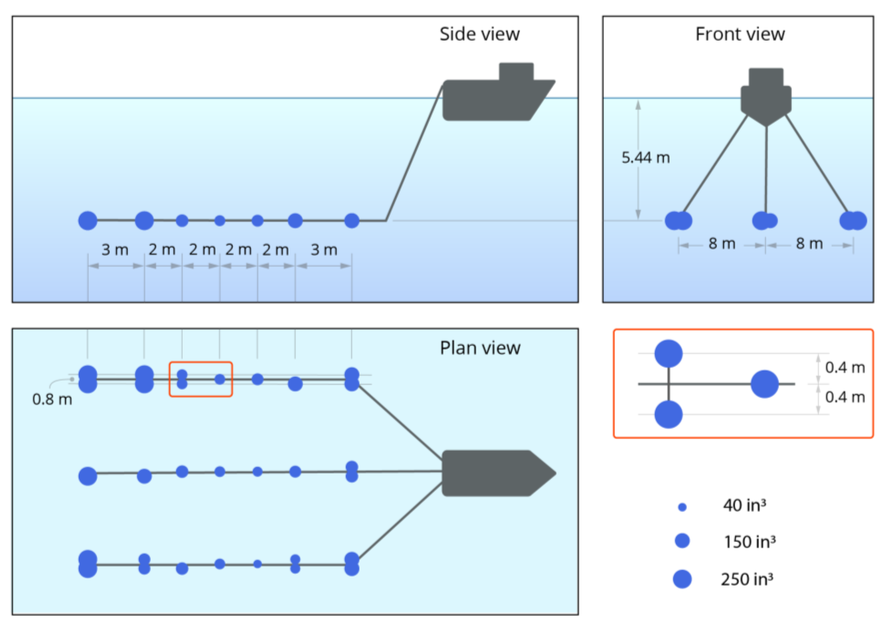
| 1 | Transition Zone (Java Sea) | July | 10–25 | 100 | 25,000 | 12,290 cm3 (750 in3) | 18 elements, 15 × 16 m |
| 2 | Shallow Water (North Sea) | August | 110–130 | 100 | 25,000 | 67,680 cm3 (4130 in3) | 18 elements, 15 × 16 m |
| 3 | 500 | ||||||
| 4 | Deep Water (Gulf of Mexico) | February | 1500–1600 | 500 | 50,000 | 67,680 cm3 (4130 in3) | 18 elements, 15 × 16 m |
| HEARING GROUP | Impulsive Source | Non-Impulsive Source |
|---|---|---|
| Low-frequency (LF) cetaceans | Lpk,flat: 219 dB LE, LF,24h: 183 dB | LE,LF,24h: 199 dB |
| Mid-frequency (MF) cetaceans | Lpk,flat: 230 dB LE,MF,24h: 185 dB | LE,MF,24h: 198 dB |
| High-frequency (HF) cetaceans | Lpk,flat: 202 dB LE,HF,24h: 155 dB | LE,HF,24h: 173 dB |
| Phocid pinnipeds (in water; PW) | Lpk,flat: 218 dB LE,PW,24h: 185 dB | LE,PW,24h: 201 dB |
| Otariid pinnipeds (in water; OW) | Lpk,flat: 232 dB LE,OW,24h: 203 dB | LE,OW,24h: 219 dB |
| Specifications | Broadside | Endfire | Vertical |
|---|---|---|---|
| SLPK (dB re 1 µPa m) | 218.6 | 218.8 | 219.1 |
| SL (dB re 1 µPa m) | 210.6 | 213.7 | 216.1 |
| ESL (dB re 1 µPa2·s m2) 0.05–0.1 kHz | 217.2 | 218.2 | 222.9 |
| ESL (dB re 1 µPa2·s m2) 0.05–1 kHz | 217.2 | 218.2 | 222.9 |
| ESL (dB re 1 µPa2·s m2) 1–25 kHz | 101.7 | 99.9 | 107.0 |
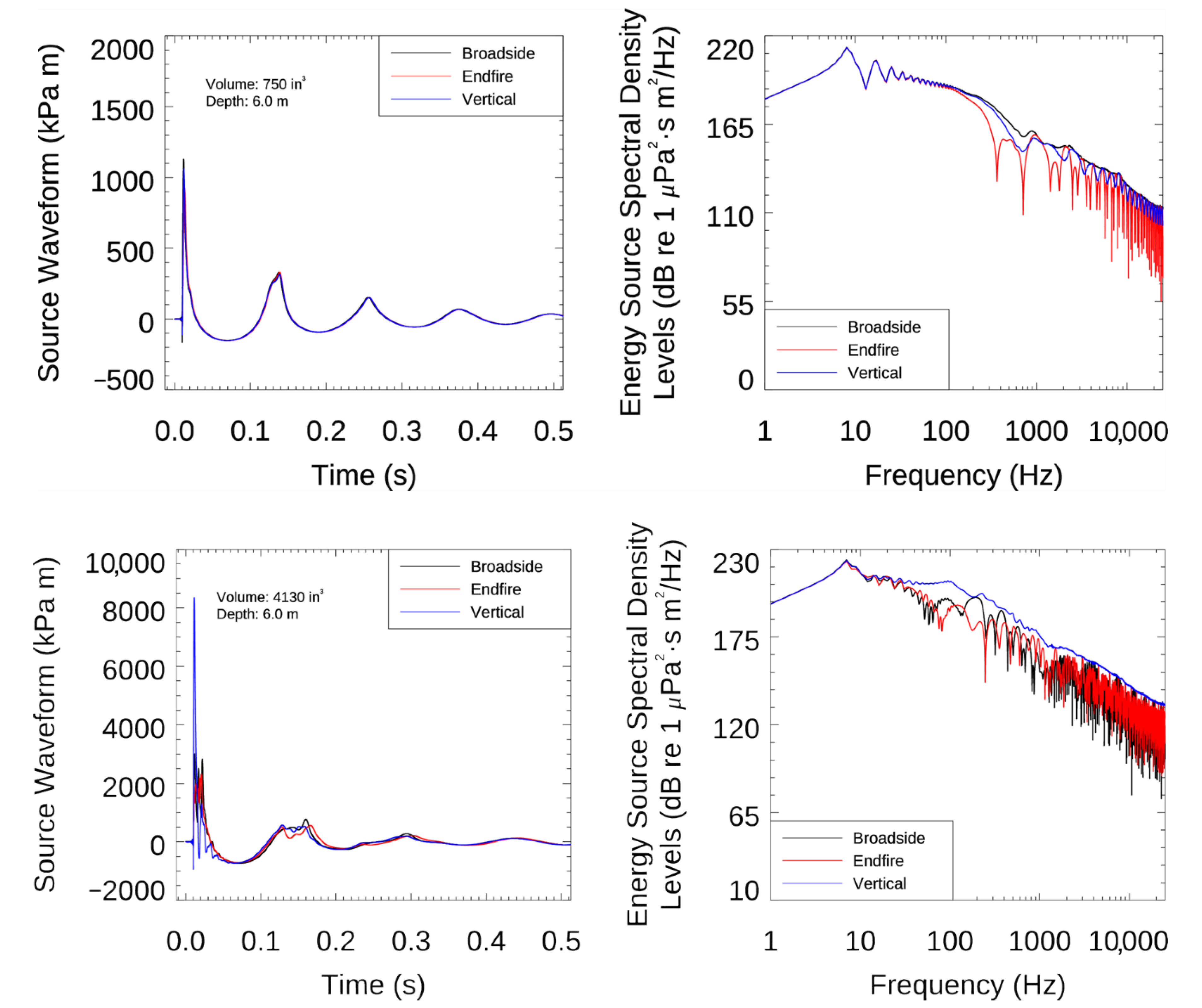
| Specifications | 12,290 cm3 (750 in3) Air Gun Array | 67,680 cm3 (4130 in3) Air Gun Array | ||||
|---|---|---|---|---|---|---|
| Broadside | Endfire | Vertical | Broadside | Endfire | Vertical | |
| SLPK (dB re 1 µPa m) | 241.1 | 239.3 | 240.5 | 249.6 | 247.3 | 258.4 |
| SL (dB re 1 µPa m) | 224.1 | 223.4 | 223.8 | 236.3 | 235.7 | 240.9 |
| ESL (dB re 1 µPa2·s m2) 0.05–0.1 kHz | 218.2 | 218.1 | 218.1 | 229.1 | 228.8 | 231.4 |
| ESL (dB re 1 µPa2·s m2) 0.05–1 kHz | 218.6 | 218.3 | 218.5 | 229.7 | 229.0 | 232.7 |
| ESL (dB re 1 µPa2·s m2) 1–25 kHz | 182.9 | 179.6 | 181.3 | 187.2 | 191.1 | 199.9 |
| Depth Regime | Depth (m) | Density (g/cm3) | P-Wave Speed (m/s) | P-Wave Attenuation(dB/λ) | S-Wave Speed (m/s) | S-Wave Attenuation(dB/λ) |
|---|---|---|---|---|---|---|
| Transition Zone | 0–5 | 1.5–1.6 | 1500–1535 | 0.16–0.26 | 150 | 3.6 |
| 5–10 | 1.6–1.7 | 1535–1565 | 0.26–0.32 | |||
| 10–20 | 1.7–1.8 | 1565–1630 | 0.32–0.37 | |||
| 20–50 | 2.2 | 1800–1900 | 0.8–1.1 | |||
| 50–100 | 2.2 | 1900–2150 | 1.1–1.6 | |||
| 100–250 | 2.2 | 2150–2300 | 1.6–2.0 | |||
| 250–500 | 2.2 | 2300–2625 | 2.0–2.3 | |||
| >500 | 2.2 | 2625 | 2.3 | |||
| Shallow Water | 0–50 | 1.70–1.95 | 1550–1650 | 0.60–0.82 | 150 | 3.0 |
| 50–700 | 1.95–2.20 | 1650–1800 | 0.82–0.8 | |||
| >700 | 2.40 | 2200 | 0.2 | |||
| Deep Water | 0–50 | 1.5–1.6 | 1500–1550 | 0.14–0.42 | 100 | 0.1 |
| 50–180 | 1.6–1.8 | 1550–1670 | 0.42–0.50 | |||
| 180–250 | 1.8–2.0 | 1670–1900 | 0.50–1.70 | |||
| 250–1000 | 2.0–2.5 | 1900–2200 | 1.70 | |||
| >1000 | 2.5 | 3000 | 0.20 |
| Hearing Group [13] | Transition Zone | Shallow Water | Deep Water |
|---|---|---|---|
| Low-frequency (LF) cetaceans | Humpback whale (Megaptera novaeangliae) | Minke whale (Balaenoptera acutorostrata) | Bryde’s whale (Balaenoptera edeni) |
| Mid-frequency (MF) cetaceans | Bottlenose dolphin (Tursiops truncates) | Bottlenose dolphin White-beaked dolphin (Lagenorhynchus albirostris) | Bottlenose dolphin Sperm whale (Physeter macrocephalus)Cuvier’s beaked whale (Ziphius cavirostris) |
| High-frequency (HF) cetaceans | Finless porpoise (Neophocaena phocaenoides) | Harbor porpoise (Phocoena phocoena) | Pygmy sperm whale (Kogia breviceps) |
| Phocid pinnipeds (in water; PW) | N/A | Harbor seal (Phoca vitulina) | N/A |
| Scenario | Species Name | MV Array | Air Gun Array | |
|---|---|---|---|---|
| SEL | PK | SEL | ||
| 1 | Humpback whale | <0.01 | <0.01 | 0.03 |
| Bottlenose dolphin | <0.01 | 0.07 | <0.01 | |
| Finless porpoise | <0.01 | 24.07 | <0.01 | |
| 2 | Minke whale | <0.01 | 0.26 | 0.45 |
| Bottlenose dolphin | <0.01 | <0.01 | <0.01 | |
| White-beaked dolphin | <0.01 | 0.01 | <0.01 | |
| Harbor porpoise | <0.01 | 12.9 | 0.10 | |
| Harbor seal | <0.01 | 0.08 | 0.08 | |
| 3 | Minke whale | <0.01 | 0.27 | 0.47 |
| Bottlenose dolphin | <0.01 | <0.01 | <0.01 | |
| White-beaked dolphin | <0.01 | 0.01 | <0.01 | |
| Harbor porpoise | <0.01 | 13.6 | 0.06 | |
| Harbor seal | <0.01 | 0.13 | 0.06 | |
| 4 | Bryde’s whale | <0.01 | <0.01 | <0.01 |
| Sperm whale | <0.01 | <0.01 | <0.01 | |
| Bottlenose dolphin | <0.01 | <0.01 | <0.01 | |
| Cuvier’s beaked whale | <0.01 | <0.01 | <0.01 | |
| Pygmy sperm whale | <0.01 | <0.01 | <0.01 | |
| Scenario | Species Name | Step Function Thresholds | Single-Value Thresholds | ||
|---|---|---|---|---|---|
| MV Array | Air Gun Array | MV Array | Air Gun Array | ||
| 1 | Humpback whale | 0.06 | 0.08 | 0.09 | 0.09 |
| Bottlenose dolphin | 2.95 | 8.89 | 23.1 | 13.9 | |
| Finless porpoise | 107 | 239 | 266 | 172 | |
| 2 | Minke whale | 1.76 | 15.3 | 44.2 | 23.6 |
| Bottlenose dolphin | 0.01 | 0.08 | 0.24 | 0.12 | |
| White-beaked dolphin | 0.20 | 3.05 | 7.82 | 5.33 | |
| Harbor porpoise | 26.4 | 175 | 113 | 64.3 | |
| Harbor seal | 0.23 | 1.32 | 3.84 | 1.95 | |
| 3 | Minke whale | 1.75 | 15.6 | 45.8 | 23.9 |
| Bottlenose dolphin | 0.02 | 0.14 | 0.38 | 0.22 | |
| White-beaked dolphin | 0.17 | 3.21 | 8.40 | 5.72 | |
| Harbor porpoise | 28.7 | 183 | 120 | 68.9 | |
| Harbor seal | 0.24 | 1.50 | 4.23 | 2.30 | |
| 4 | Bryde’s whale | <0.01 | 0.05 | 0.28 | 0.05 |
| Sperm whale | 0.03 | 0.70 | 6.89 | 1.24 | |
| Bottlenose dolphin | <0.01 | <0.01 | 0.20 | <0.01 | |
| Cuvier’s beaked whale | 0.05 | 0.62 | 0.81 | 0.12 | |
| Pygmy sperm whale | <0.01 | <0.01 | 0.92 | <0.01 | |
Publisher’s Note: MDPI stays neutral with regard to jurisdictional claims in published maps and institutional affiliations. |
© 2020 by the authors. Licensee MDPI, Basel, Switzerland. This article is an open access article distributed under the terms and conditions of the Creative Commons Attribution (CC BY) license (http://creativecommons.org/licenses/by/4.0/).
Share and Cite
Matthews, M.-N.R.; Ireland, D.S.; Zeddies, D.G.; Brune, R.H.; Pyć, C.D. A Modeling Comparison of the Potential Effects on Marine Mammals from Sounds Produced by Marine Vibroseis and Air Gun Seismic Sources. J. Mar. Sci. Eng. 2021, 9, 12. https://doi.org/10.3390/jmse9010012
Matthews M-NR, Ireland DS, Zeddies DG, Brune RH, Pyć CD. A Modeling Comparison of the Potential Effects on Marine Mammals from Sounds Produced by Marine Vibroseis and Air Gun Seismic Sources. Journal of Marine Science and Engineering. 2021; 9(1):12. https://doi.org/10.3390/jmse9010012
Chicago/Turabian StyleMatthews, Marie-Noël R., Darren S. Ireland, David G. Zeddies, Robert H. Brune, and Cynthia D. Pyć. 2021. "A Modeling Comparison of the Potential Effects on Marine Mammals from Sounds Produced by Marine Vibroseis and Air Gun Seismic Sources" Journal of Marine Science and Engineering 9, no. 1: 12. https://doi.org/10.3390/jmse9010012
APA StyleMatthews, M.-N. R., Ireland, D. S., Zeddies, D. G., Brune, R. H., & Pyć, C. D. (2021). A Modeling Comparison of the Potential Effects on Marine Mammals from Sounds Produced by Marine Vibroseis and Air Gun Seismic Sources. Journal of Marine Science and Engineering, 9(1), 12. https://doi.org/10.3390/jmse9010012