Effect of Residual Stresses on the Elastoplastic Behavior of Welded Steel Plates

Abstract

A robust methodology to simulate virtually the residual stresses pattern in welded steel plates is presented. The methodology is applied to the structural analysis of typical welded plates belonging to ship structures, and the effect of residual stresses on the elastoplastic behavior of plates loaded axially is analyzed in comparison to the residual stress free case, both for tension and compression and including initial imperfections. Residual stresses affect in different manner plates with different geometries; thus a parametric study is performed covering the usual range of variation of the most important plate parameters that control the strength of the plates, more precisely the slenderness and the aspect ratio. The results from finite elements analysis are compared with codes and most established formulations and recommendations of applicability in the prediction of load-shortening curves for hull’s bending strength evaluation, ultimate strength and ultimate strain of plate elements are made.

1. Introduction

The study of unstiffened plates under different loading conditions has been object of very deep and extensive analysis along time in relation to the effect of the most important parameters that influence the ultimate strength of such plates.

Plate elements are a fundamental component of stiffened plates that are the basis of structural strength of thin-walled structures evaluation. The hull girder of a ship is subjected to different loadings, like bending moment, shear force and lateral pressure. Plate elements are very important in all cases contributing greatly to resist those loadings. In the particular case of the hull girder strength assessment, the structure may be considered to be formed by a set of stiffened plates each of them contributing to resist the applied bending moment and other loads [1,2,3]. The response of each stiffened element depends greatly from the contributions of the associated plate attached to the stiffeners and frames [4].

The evaluation of the residual stresses distribution along the structure has been concentrated in three main fields: development of non-destructive and destructive techniques [5], use of finite element methods and analytical studies associated with the mechanical characteristics of the different material and welding techniques. Leggatt [6] explains the residual stresses in welded structures, i.e., how the different factors affect the magnitude, direction and distribution of residual stresses in welded joints and structures. There exist today several commercial finite elements (FE) codes that may be employed for detailed nonlinear simulations of the development of the temperature and stress fields present during welding.

Lindgren [7], Runesson et al. [8] and Dong [9] discussed methods for numerical simulation of the welding process taking into consideration actual thermal, mechanical and microstructure developments. The focus is on material modelling, coupling effects between thermal, mechanical fields and microstructure, numerical techniques and modelling aspects.

The evaluation of the residual stresses level in 3-D structures may be done indirectly. It requires the imposition of some hypotheses to establish the residual stress pattern and may be obtained by two methods: the structural tangent modulus method and the total energy dissipation method [10]. The first one considers the variation of the tangent modulus under alternate loading at a point of a cycle corresponding to the maximum loading point in the previous cycle. The variation of the tangent modulus is the result of the variation on the effective inertia of the section due to the development of local plasticity at points where residual stresses are still high. The second method considers the dissipation of energy in a structure with residual stresses when an external load is applied [11].

Tekgoz et al. [12] analyzed the effect of residual stress on the ultimate strength assessment of a stiffened panel by a nonlinear finite element method. They develop modified stress strain curves in order to include a model of residual stresses on material properties. An improved approach was proposed by Launert et al. [13] by prescribing initial deformations and simplified residual stress pattern manually in the numerical model applied to welded plate girders. The present methodology allows to implement residual stresses in direct way by using the concept of heat affected zone (HAZ) and mechanical and thermal properties of the material.

2. Methodology

This work studies the effect of residual stresses on the behavior of unstiffened rectangular plates subjected to axial compression. In order to achieve this objective, a methodology to implement residual stresses in structural plate elements due to welding process is presented. The internal state of stresses obtained in this first stage is used as initial condition for the evaluation of the unstiffened plate structural performance by finite element analysis.

2.1. Implementation of Residual Stresses due to Welding

The plate elements are divided into different regions according to the thermal process that they are subjected during the welding process. A typical plate element belonging to a ship’s panel has a length a and a width b and is welded on its borders to stiffeners and frames, thus there are strips of the plate in the borders that suffer the effect of heating and cooling during the welding process, developing permanent plastic strains that affect the initial internal state of stresses in the whole plate in the end of the welding process.

2.1.1. Theoretical Model of Residual Stresses for Perfect Plates

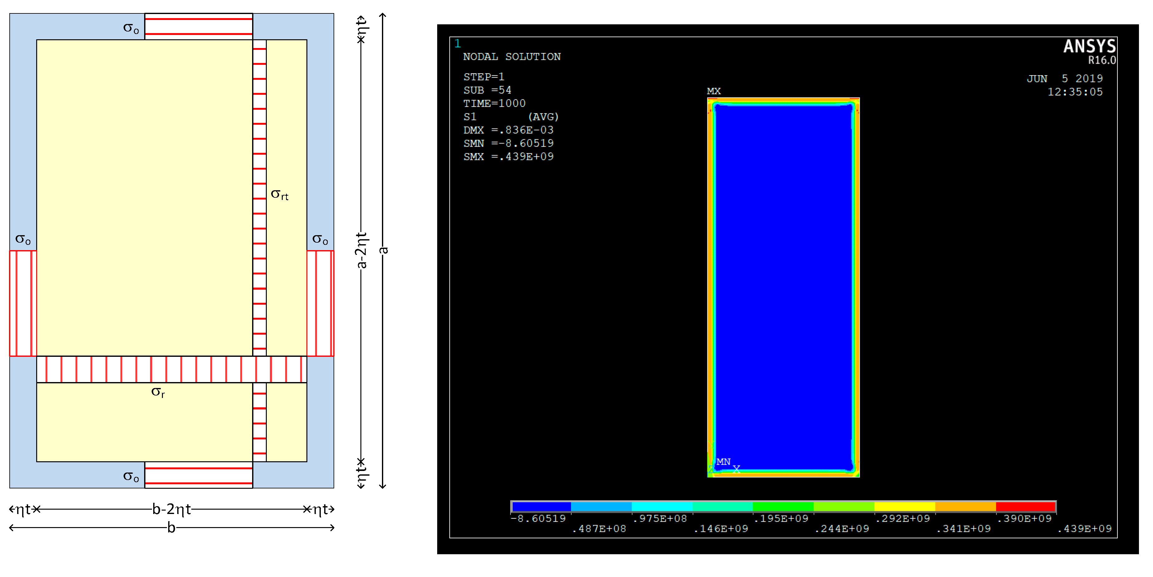
It is commonly accepted that these residual stresses patterns may be simply represented by a strip of plate near each border with a width ηt at yield stress (${\sigma }_o$) in tension and a central region under compression at a stress ${\sigma }_r$ with a width of b-2ηt that equilibrates the plate. η is the factor that relates the width of the heat affected zone with the thickness of the plate t.

The equilibrium equation of loads for the plate quantifies the residual stress as:

$${\sigma }_r=-{\sigma }_o\frac{2\eta t}{b-2\eta t}$$

(1)

In the transverse direction the transversal residual stress in the middle of the plate is:

$${\sigma }_{rt}=-{\sigma }_o\frac{2\eta t}{a-2\eta t}$$

(2)

Figure 1 presents the distribution of residual stresses in the flat plate, after welding, both in longitudinal and transversal directions, for the simplified approach (left) [11] and the one obtained by thermal analysis (right) [14]. A similar approach was present by Yi et al. [15] to represent the biaxial state of residual stresses in welded panels.

2.1.2. Implementation of Residual Stresses by FE Modelling

The study of plates with initial residual stresses requires, as a first step, the introduction of the residual stresses pattern as described in Figure 1. There are several ways to achieve such objective [16,17,18], some of them very complex and computationally costly.

The present method allows to perform the thermal analysis to introduce residual stresses, followed by structural analysis without intermediate steps and been computationally very efficient.

The plate model in finite elements (FE) is divided by parts as described in Figure 1 where the lateral strips representing the heat affected zone (HAZ) have a width ηt. The characterization of the material for such analysis requires in general the information about the mechanical properties for different temperatures and the respective coefficient of thermal expansion.

The present method only uses the modulus of elasticity, the yield stress at room temperature and the respective coefficient of thermal expansion, considering an elastic-perfectly plastic deformation without hardening. The thermal loading is inputted by rising the temperature into the HAZ strips to a reference temperature, in this study 500 °C, followed by a decrease to room temperature, while the temperature in the rest of the plate is kept at room temperature during the whole process [14].

In the first step, the temperature rises to 500 °C in HAZ and it generates plasticity in compression in the lateral strips and some tensile stresses in the central part of the plate. During the second step, cooling of the HAZ strips, the state of internal stresses reverses and, in the end, one has tensile yield stress in the lateral strips and residual compressive stresses in the central part.

This simplified procedure allows to obtain the required residual stress pattern and proceed directly to a structural analysis in a sequential FE analysis load step. It is recommended to use a mesh size less than half of the HAZ width, preferably ηt/3. The peak temperature needs to be bigger than a reference value given by:

$$\Delta T=\frac{2{\sigma }_o}{{\alpha }_{T}E}$$

(3)

which is the minimum difference of temperature required to pass from yield stress in compression to yield stress in tension on HAZ strips. For mild steel, reference values in equation are ${\sigma }_o$ of 240 MPa, E is 210 GPa and the coefficient of thermal expansion ${\alpha }_T$ is 1.1 × 10⁻⁵ K⁻¹ resulting in a minimum difference of temperatures $\Delta T$ of 208 °C.

2.1.3. Implementation of Procedure in FE Modelling

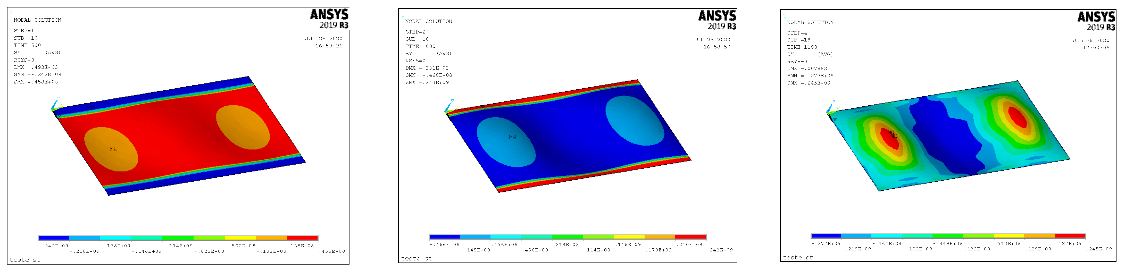
The complete procedure is composed by four stages: 1. Heating of HAZ strips up to 500 °C; 2. Cooling of HAZ strips down to room temperature (T = 20 °C); 3. Initial shortening; 4. Compressive displacement in top of plate up to collapse and beyond. The full procedure is presented in Figure 2.

The step 3 is not mandatory but it is very important and it guarantees that part of the residual stresses are not dissipated in the beginning of step 4. Its value must be bigger than the residual longitudinal displacement at the top in the end of thermal analysis, step 2, and the structural analysis on this step 3 should be performed without sub-steps. In more detail and taking as example a plate with residual stresses ${\sigma }_r$ after the thermal analysis, one has a residual longitudinal shortening in the end of step 2 given by ${\sigma }_r/E·a$. If the initial increment of displacement in the structural analysis is smaller than the residual shortening, the plate suffers residual stresses relaxation by plasticity in tensile strips with a decrease in the level of residual stresses. So one should guarantees that the initial increment of load avoids this in the structural analysis. In this work, it decided to do it independently (step 3) and restart the analysis from that point with better control of the increment of load (step 4).

Figure 3 shows the distribution of stresses in the end of steps 1, 2 and at collapse in step 4 for the top layer. As it can be seen, in the end of 1st step the HAZ strips are in compression at yield stress while they are in tension after plasticity in the end of the 2nd step. In the whole process the residual stress pattern varies from point to point due to the presence of initial imperfections and deformations developed during the loading.

The commercially available finite element software ANSYS [19] has been used for this study. Eight-node shell elements SHELL281 are used which are well-suited for large strain nonlinear applications. Full Newton-Raphson solution procedure was implemented to perform the nonlinear finite element analysis. The mesh of each plate was associated with the tensile strip width as mentioned previously, mesh size less than half of the HAZ width, preferably ηt/3 in order to obtain a reliable representation of residual stresses pattern.

2.2. Parameters Affecting the Strength of Unstiffened Plates

The parameters that most affect the structural behavior in compression, represented by the load-shortening curves (LSC), and the ultimate strength, are the plate slenderness, initial geometric imperfections, residual stresses, boundary conditions and complexity of loading.

2.2.1. Plate Slenderness

The definition of the plate slenderness β results directly from the resolution of rectangular plate’s buckling formulation where the elastic critical Euler’s stress of a plate under axial compression is:

$$\frac{{\sigma }_{cr}}{{\sigma }_o}=k_{cr}\frac{{\pi }^2}{12\left(1-{\nu }^2\right){\beta }^2}$$

(4)

β considers both the geometry of the plate and its material properties and is given by Equation (5) while $k_{cr}$ accounts for the mode of buckling having as minimum 4 when m = a/b.

$$\beta =\frac{b}{t}\sqrt{\frac{{\sigma }_o}{E}}$$

(5)

$$k_{cr}={\left(\frac{mb}{a}+\frac{a}{mb}\right)}^2$$

(6)

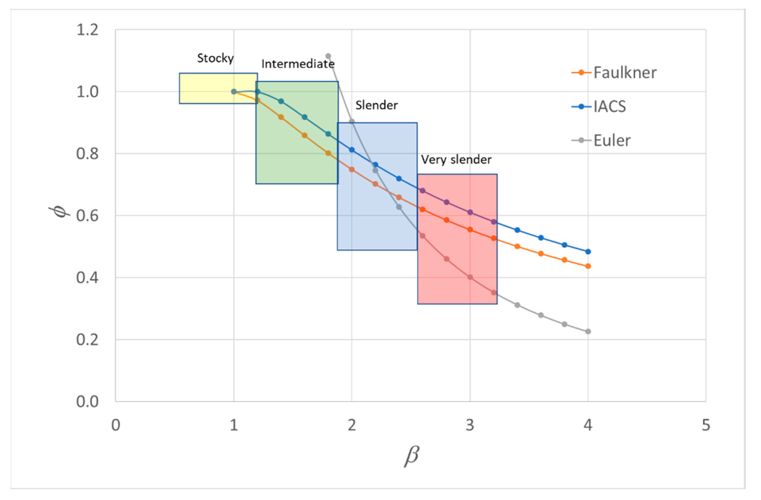
When the critical stress approaches or overlaps the yield stress, some plasticity is developed in some points of the plate and the ultimate stress of the plate becomes less than the critical one. Several proposals have been presented in the past to estimate the ultimate strength, some of them having the plate slenderness as unique parameter. Two important examples are Faulkner’s (Equation (7)) and Frankland’s (Equation (8)) equations that are used as well to introduce the concept of effective width. The former is representative of the strength of simply supported welded plates [20] and the latter is used in International Association of Classification Societies (IACS) formulation in the definition of the effective width of the attached plate in a stiffened structural element [3,21].

$${\varphi }_u=\frac{{\sigma }_u}{{\sigma }_o}=\frac{2}{\beta }-\frac{1}{{\beta }^2}\left(for\beta >1\right)$$

(7)

$${\varphi }_u=\frac{{\sigma }_u}{{\sigma }_o}=\frac{2.25}{\beta }-\frac{1.25}{{\beta }^2}\left(for\beta >1.25\right)$$

(8)

Figure 4 compares these formulas showing that IACS equation predicts higher strength under in-plane compression than Faulkner’s approach, which is eventually a consequence of the effect of residual stresses on the strength of the plates used in the database. It also presents in the same figure a qualitative classification of unstiffened plates according to relative importance of plasticity and elastic instability on the behavior and strength of the plates, as follows: stocky plates, dominated by plasticity and yield stress; intermediate plates, where elastoplastic effects are very important with a critical stress above yield stress; slender plates, having high degradation of the ultimate strength with increase of slenderness and a critical stress above 0.5 yield stress: and very slender plates with very low ultimate strength due to very low critical stress. The range of slenderness covered in this classification is the most common in ship’s structures, which varies from 1 to 2.5 according Zhan [22].

2.2.2. Geometric Imperfections

Several studies [23,24,25,26,27,28,29] proposed different values and formulas to estimate the amplitude of initial imperfections, most of them pointing out to the maximum value without consideration to the mode of imperfections.

In this work a reference value given by Equation (9) is considered and a wide range of amplitude around that value is used to estimate the relevancy of the parameter.

$$\frac{w_i}{t}=0.1{\beta }^2$$

(9)

Different amplitudes and modes of imperfections are considered, corresponding to the expansion of the shape of imperfections into Fourier series that can be represented by:

$$\mathrm{w}\left(x,y\right)=\sum \sum w_i.sin\frac{m\pi x}{a}.sin\frac{\pi y}{b}$$

(10)

The importance of the mode of imperfections is analyzed by considering the fundamental mode (m = 1) which normally leads to stronger plates, and the critical one corresponding to the weaker plate. Since a/b is 2.5 in the models of this study, the critical mode m is 3.

2.2.3. Boundary Conditions

The adoption of appropriate boundary conditions (BC) on each type of structure is of vital importance because the differences on structural behavior and strength can be very large between them. A plate element works normally associated with stiffeners and frames and its contribution to the strength of the structure depends on the restraining action of these elements, both in terms of displacements and rotations.

One may consider 4 main classes of boundary conditions for plate elements belonging to panels:

• Unrestrained; all lateral edges and tops, respectively long and short edges in a rectangular plate, are supported perpendicularly to the plate’s plane, but in-plane movements along the lateral edges are allowed and rotations are free.
• Restrained; all lateral edges and tops are supported perpendicularly to the plate’s plane, but in-plane movements along the edges are not allowed, called as fixed condition, and rotations are free.
• Constrained; all lateral edges and tops are supported perpendicularly to the plate plane, in-plane movements of the lateral edges are allowed but kept straight and rotations are free.
• Clamped; displacements and rotations are null in all edges.

Each of the above classes leads to differences on the load-elongation curves, ultimate strength and ultimate strain, modes of collapse both in compression and tension. In terms of ultimate strength, the difference may be bigger than 20% in compression, leading to completely different modes of collapse due to the development of transversal stresses induced by Poisson effect [30,31].

Unrestrained and constrained conditions guarantee that the loading in uniaxial compression do not generate globally transversal loading in the lateral edges. Restrained conditions generate a biaxial state of stresses leading normally to stronger response of the plate, with higher ultimate strength and difference collapse mode in certain cases [30]. Clamped conditions can be representative for very rigid framing system in panels, which is not usual in ship’s structures, at least on the hull girder.

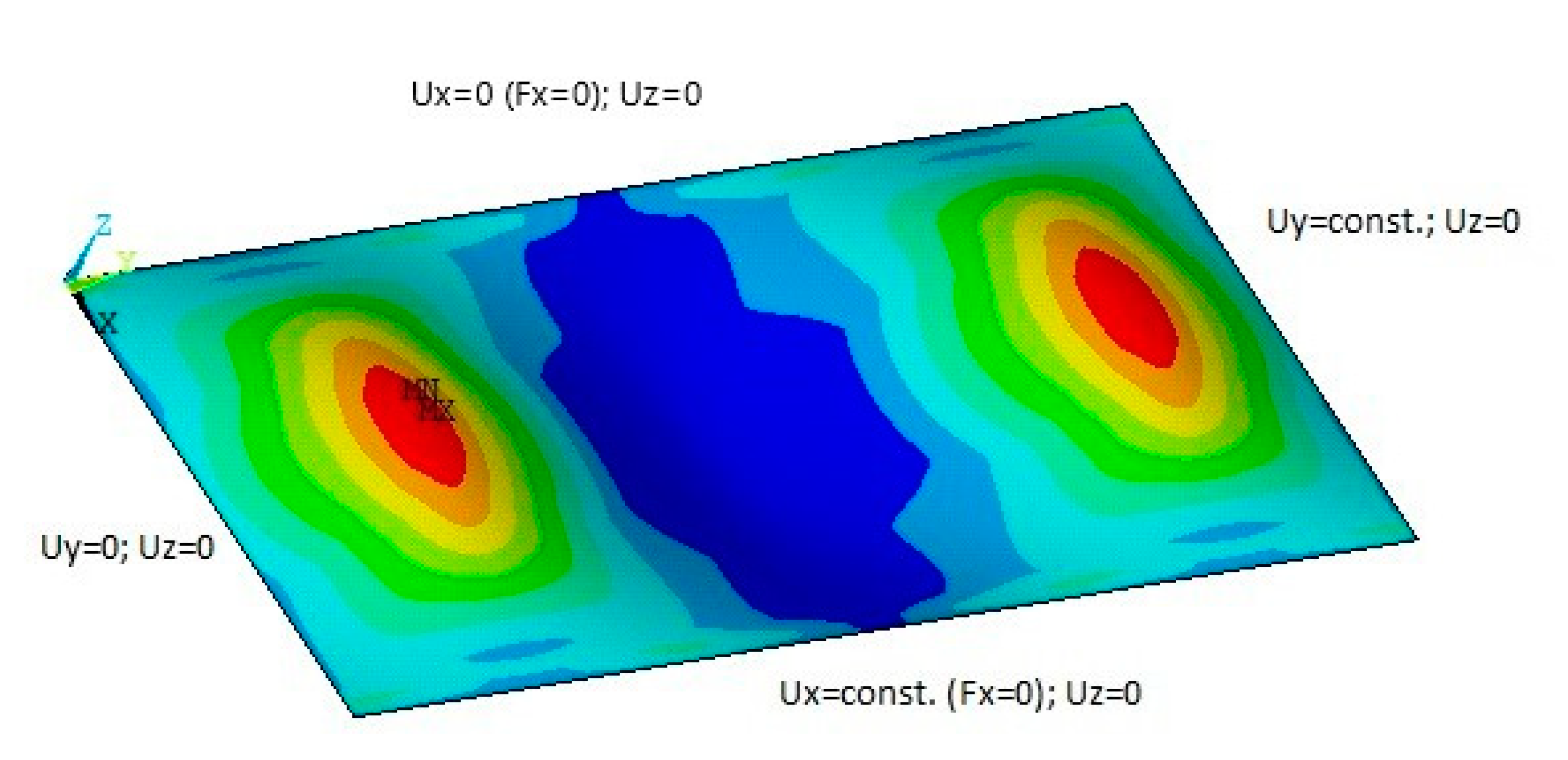
Due to the nature of stiffening on ship’s panels, it is considered that the constraint condition is the most appropriate to represent the behavior of plate elements belonging to ship’s structures. Unrestrained are rather conservative and restrained conditions are too optimistic. Figure 5 shows the boundary conditions on the FE model used in this study.

The rectangular plate is loaded longitudinally in y direction applying a displacement (Uy) on the right top edge, that remains straight; the left top is fixed (Uy = 0). The upper lateral edge is fixed in the direction perpendicular to the loading (Ux = 0) and the lower lateral edge remains straight but it is free to move in-plane, Ux = constant for each load step, satisfying the condition of a null total net load in the lateral edges during the load path (Fx = 0). These BC’s guarantee a pure uni-axial loading of the plate. Similar BC for the plate element were used by Li et al. [32] in the study of ultimate compressive strength of welded stiffened plates.

3. Results

The analysis of the influence of residual stresses on plate’s behavior is performed by FE analysis considering a rectangular plate with length a of 1.5 m and a width b of 0.6 m resulting in an aspect ratio α of 2.5 as the basic model.

Four different thicknesses of the plate are considered: 20, 15, 10 and 8 mm. These thicknesses are representative of different classes of plates in terms of elastoplastic behavior and buckling, respectively stocky, intermediate, slender and very slender plates with increase in the elastic instability in compression. The width to thickness ratio, b/t, is respectively 30, 40, 60 and 75.

At least 2 levels of initial geometric imperfections are considered for each group in order to evaluate its effect on the degradation of the ultimate strength in compression. Since the plate’s structural behavior is very sensitive to the mode of initial imperfections, 2 modes are considered and compared, the fundamental (m = 1) and the critical one (m = 3).

The material is considered to have an elastic, perfectly plastic behavior with a Young modulus E of 210 GPa and yield stress, ${\sigma }_o$, of 240 MPa.

The boundary conditions in this study are simply supported in all edges. The edges remain straight during the loading path and the net load in the lateral edges is null, which means that the loading is globally uniaxial, and a global transversal movement of lateral edges is allowed (constrained condition).

3.1. Stocky Plates

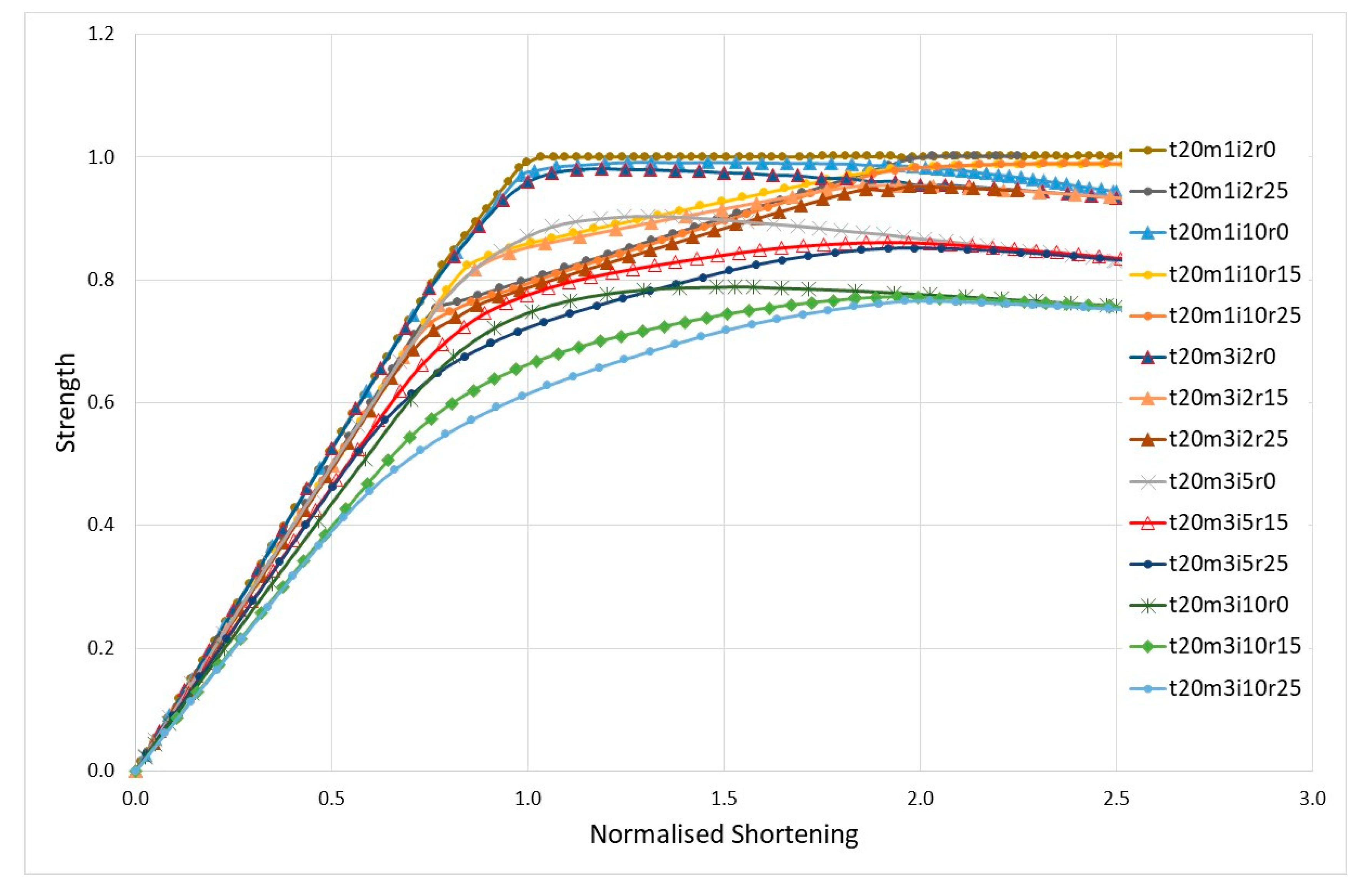
In this group the plates have a slenderness β of 1.014 (b/t = 30). The reference value for the initial imperfections of these plates, w_i, is 2 mm according to Equation (9). Three different levels of imperfections are considered: 2, 5 and 10 mm, which corresponds to w_i/t ratio of 0.1, 0.25 and 0.5, respectively. Two modes of imperfections are analyzed: the fundamental, m = 1, and the critical one, m = 3. The effect of residual stresses for each plate is evaluated for three levels of width of the tensile strip at the edges: η = 0, 2 and 3 to which corresponds a normalized residual stress level of 0.0, 0.15 and 0.25.

The load shortening curves are presented in Figure 6, where the strength is the average compressive stress normalized by the yield stress. The results of the ultimate strength and the corresponding strain normalized by yield strain are presented in

Table 1. Summary of data and main results for plates with a = 1.5 m, b = 0.6 m and t = 20 mm.

Identification	Mode i	wi (mm)	wi/t	η	Ultimate Stress	Ultimate Strain	Residual Stress %
t20m1i2r0	1	2	0.10	0	1.001	1.00	0.00
t20m1i2r25	1	2	0.10	3	1.002	2.00	0.25
t20m1i10r0	1	10	0.50	0	0.991	1.46	0.00
t20m1i10r15	1	10	0.50	2	0.989	2.36	0.15
t20m1i10r25	1	10	0.50	3	0.990	2.37	0.25
t20m3i2r0	3	2	0.10	0	0.982	0.98	0.00
t20m3i2r15	3	2	0.10	2	0.954	1.94	0.15
t20m3i2r25	3	2	0.10	3	0.952	1.97	0.25
t20m3i5r0	3	5	0.25	0	0.904	1.31	0.00
t20m3i5r15	3	5	0.25	2	0.861	1.92	0.15
t20m3i5r25	3	5	0.25	3	0.851	1.99	0.25
t20m3i10r0	3	10	0.50	0	0.789	1.53	0.00
t20m3i10r15	3	10	0.50	2	0.772	1.94	0.15
t20m3i10r15	3	10	0.50	3	0.765	2.03	0.25

for the different cases.

The analysis of the curves and their maximum values allows to withdraw several conclusions.

Plates with fundamental mode (m = 1) have a behavior very similar to material behavior and do not suffer almost any degradation of strength with the increase of amplitude of the imperfections. The ultimate strength maintains constant for large shortening. Residual stresses change the shape of residual stress free LSC in the range of normalized shortening from 1 − σ_r/σ_o to 2 by an almost straight cut. The ultimate stress passes to occur at normalized ultimate shortening of 2.

One the other hand, plates with critical mode (m = 3) suffer a large degradation of strength with the increase of the amplitude of initial imperfections. Nevertheless, the less imperfect one (w_i = 2 mm) has an ultimate strength close to the values found in plates with fundamental mode of imperfections.

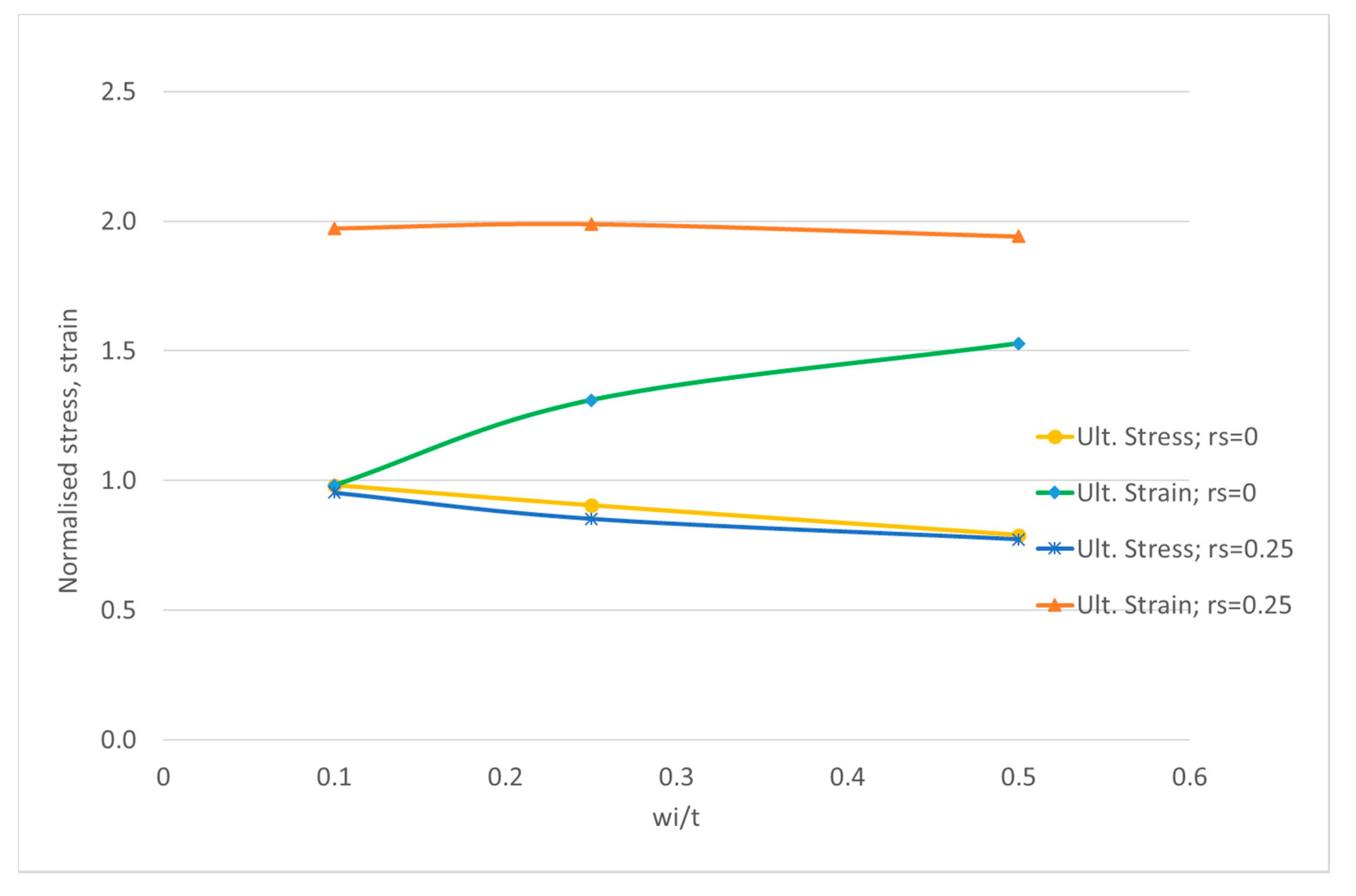
The degradation of the ultimate strength due to increase on amplitude of imperfections is very important for this group of plates (m = 3) and the ultimate strength can be quantified as:

$${\varphi }_u\left(\beta =1.01;rs=0\%\right)=1.027-0.479\frac{w_i}{t}$$

(11)

The ultimate strain of the residual stresses free plate also suffers a shift with the increase of the amplitude of initial imperfections towards a normalized strain of 1.5, as shown in Figure 7.

Residual stresses have a similar effect to the one descripted previously for plate with m = 1 by cutting the LSC to lower values in the same range of shortening. Finally, initial imperfections and residual stress seems to reduce the structural modulus of the plate in elastic range given by the slope of LSC in Figure 6. The ultimate normalized strain in plates with residual stresses is close to 2, which is the limit of the effect of the tensile strips due to welding.

The load-shedding pattern, after the ultimate load on plates with residual stresses, follows the path of the similar residual stress free plate.

The ultimate strength of plates with residual stresses is given by:

$${\varphi }_u\left(\beta =1.01;rs=25\%\right)=0.983-0.438\frac{w_i}{t}$$

(12)

The degradation of ultimate strength due to the level of imperfections is lower by 8.6% in the plates with residual stresses (−0.438) than in plates free of residual stresses (−0.479).

3.2. Intermediate Plates

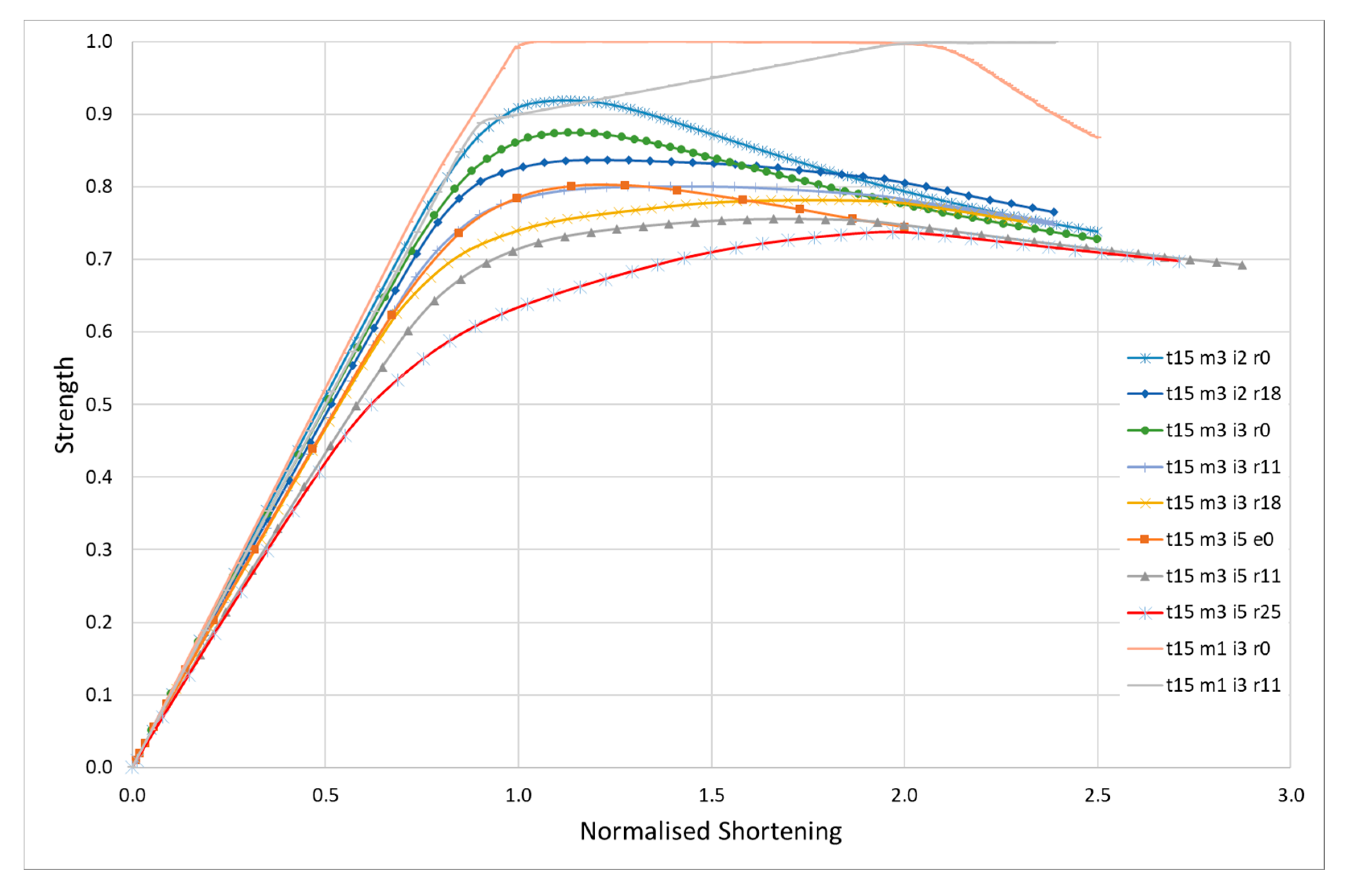
The plates in this group have a slenderness, β, of 1.352 (b/t = 40). The reference value for the initial imperfections of these plates, w_i, is 2.74 mm according to Equation (9). Three different levels of imperfections are considered: 2, 3 and 5 mm, which correspond to w_i/t ratios of 0.13, 0.2 and 0.33, respectively. The structural analysis concentrates on the critical mode, m = 3. The effect of residual stresses for each plate is evaluated for three levels of the width of the tensile strip at the edges: η = 0, 2 and 3 to which corresponds a normalized residual stress level of 0, 0.11 and 0.18.

The load shortening curves are presented in Figure 8. The results of the ultimate stress normalized by the yield stress and the corresponding strain normalized by yield strain are presented in

Table 2. Summary of data and main results for plates with a = 1.5 m, b = 0.6 m and t = 15 mm.

Identification	Mode i	wi (mm)	wi/t	η	Ultimate Stress	Ultimate Strain	Residual Stress %
t15m1i3r0	1	3	0.20	0	1.000	1.402	0.00
t15m1i3r11	1	3	0.20	2	0.999	2.114	0.11
t15m3i2r0	3	2	0.13	0	0.919	1.113	0.00
t15m3i2r18	3	2	0.13	3	0.837	1.231	0.18
t15m3i3r0	3	3	0.20	0	0.874	1.129	0.00
t15m3i3r11	3	3	0.20	2	0.801	1.449	0.11
t15m3i3r18	3	3	0.20	3	0.782	1.742	0.18
t15m3i5r0	3	5	0.33	0	0.802	1.276	0.00
t15m3i5r11	3	5	0.33	2	0.755	1.660	0.11
t15m3i5r25	3	5	0.33	4	0.737	1.969	0.25

for the different cases. The results for a plate with imperfections in the fundamental mode for comparison are also included.

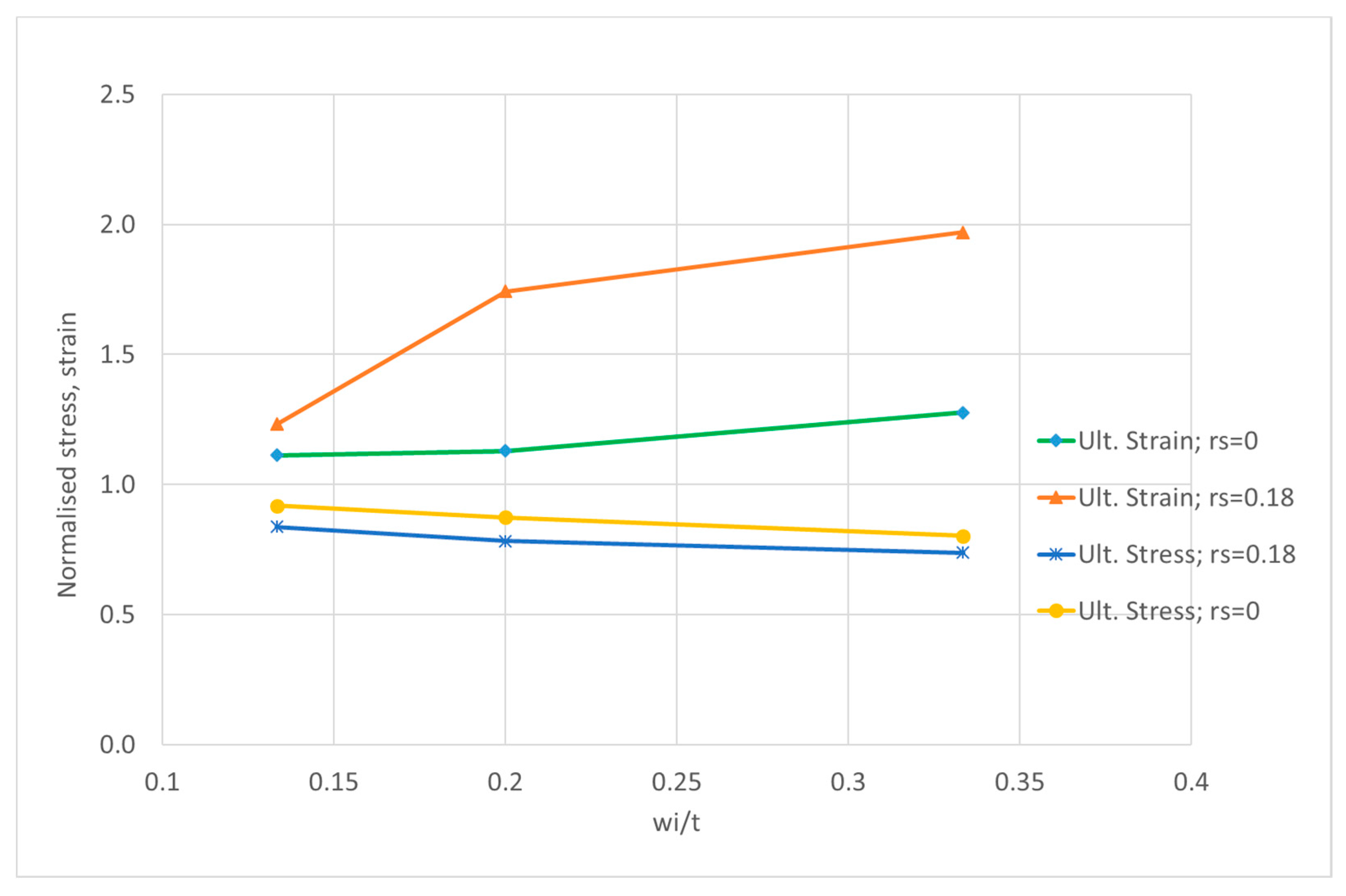
Qualitatively, the conclusions are very much in agreement with the ones described for stocky plates in relation to the increase in imperfections and residual stresses: degradation of ultimate strength, reduction of initial structural modulus and increase in ultimate strain, as it may be seen in Figure 9.

The degradation of the ultimate strength due to increase on amplitude of imperfections is even bigger than for the stocky ones for this group of plates (m = 3) and the ultimate strength of the residual stresses free plate can be quantified as:

$${\varphi }_u\left(\beta =1.35;rs=0\%\right)=0.994-0.580\frac{w_i}{t}$$

(13)

The equation for the ultimate strength for plates with residual stress of 18% of the yield stress is given by:

$${\varphi }_u\left(\beta =1.35;rs=18\%\right)=0.891-0.474\frac{w_i}{t}$$

(14)

One should note that the level of residual stresses does not affect much the ultimate strength of the plate that achieved at a normalized strain close to 2 and after that the LSC follows the residual stresses free plate LSC.

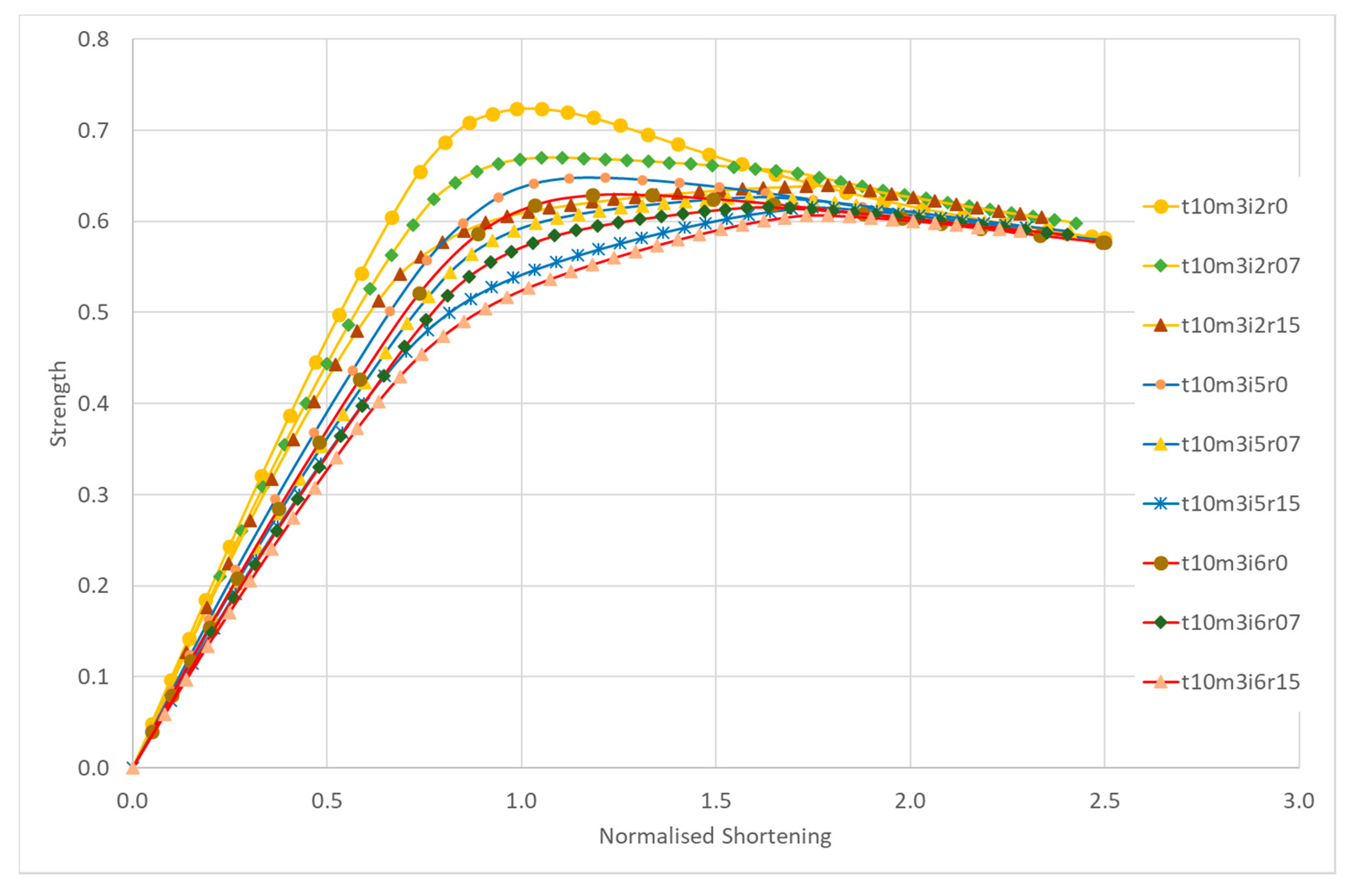
3.3. Slender Plates

The plates in this group have a slenderness β of 2.03 (b/t = 60). The reference value for the initial imperfections of these plates, w_i, is 4.11 mm according to Equation (9) corresponding to a w_i/t ratio of 0.411. Three levels of imperfections, w_i = 2, 5 and 6 mm and residual stresses of 0, 0.07 and 0.15 σ_y are considered. The LSC’s of this group of plates are shown in Figure 10.

Table 3. Summary of data and main results for plates with a = 1.5 m, b = 0.6 m and t = 10 mm.

Identification	Mode i	wi (mm)	wi/t	η	Ultimate Stress	Ultimate Strain	Residual Stress %
t10m3i2r0	3	2	0.2	0	0.724	1.052	0.00
t10m3i2r07	3	2	0.2	2	0.670	1.105	0.07
t10m3i2r15	3	2	0.2	4	0.639	1.787	0.15
t10m3i5r0	3	5	0.5	0	0.648	1.215	0.00
t10m3i5r07	3	5	0.5	2	0.626	1.641	0.07
t10m3i5r15	3	5	0.5	4	0.615	1.748	0.15
t10m3i6r0	3	6	0.6	0	0.629	1.183	0.00
t10m3i6r07	3	6	0.6	2	0.615	1.635	0.07
t10m3i6r15	3	6	0.6	4	0.606	1.733	0.15
t10m3i8r0	3	8	0.8	0	0.598	1.432	0.00
t10m3i8r15	3	8	0.8	4	0.588	1.756	0.15

presents the main results of the ultimate strength and the corresponding normalized shortening for the different cases.

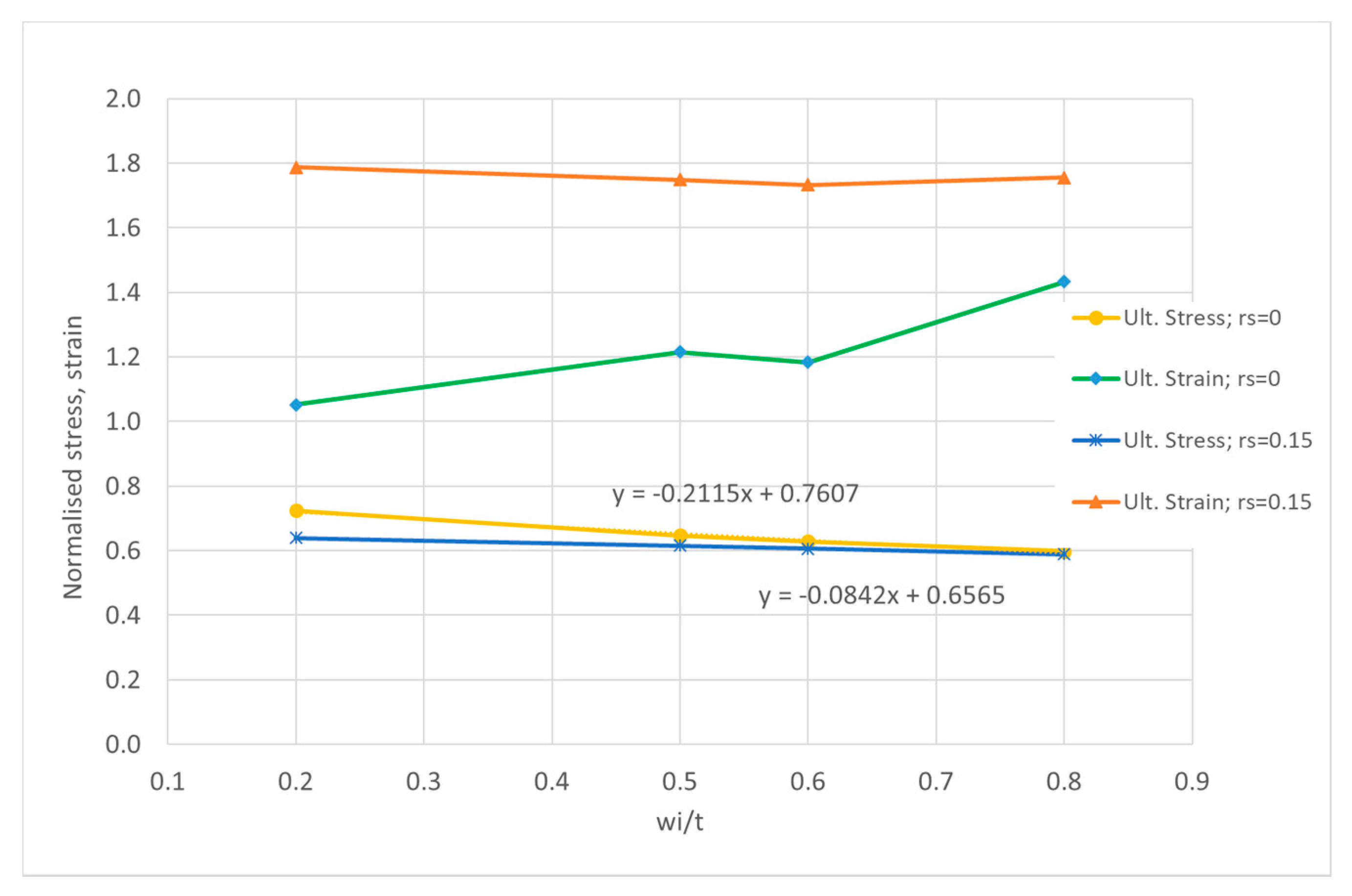
The effects of residual stresses are the reduction the initial structural modulus of the plate, the delay of collapse to normalized shortening in the range of 1.7 to 1.9, as presented in Figure 11. It is also marked the existence of the almost straight line due to the action of HAZ strips in the range 0.8–1.8 of normalized shortening.

The degradation of the ultimate strength due to increase on amplitude of imperfections is much smaller than in the previous groups, stocky and intermediate ones and the ultimate strength of residual stress-free plate can be quantified as:

$${\varphi }_u\left(\beta =2.03;rs=0\%\right)=0.761-0.212\frac{w_i}{t}$$

(15)

The ultimate strength for plates with residual stress of 15% of the yield stress is given by:

$${\varphi }_u\left(\beta =2.03;rs=15\%\right)=0.657-0.084\frac{w_i}{t}$$

(16)

Imperfections degrade the ultimate strength by a factor of 0.212 in the case of residual stress-free plate, while this factor is 0.58 in the same case for intermediate plates, which is 2.7 times more.

The ultimate strength of the plates with residual stresses is almost constant with the variation of residual stresses and initial imperfections in critical mode.

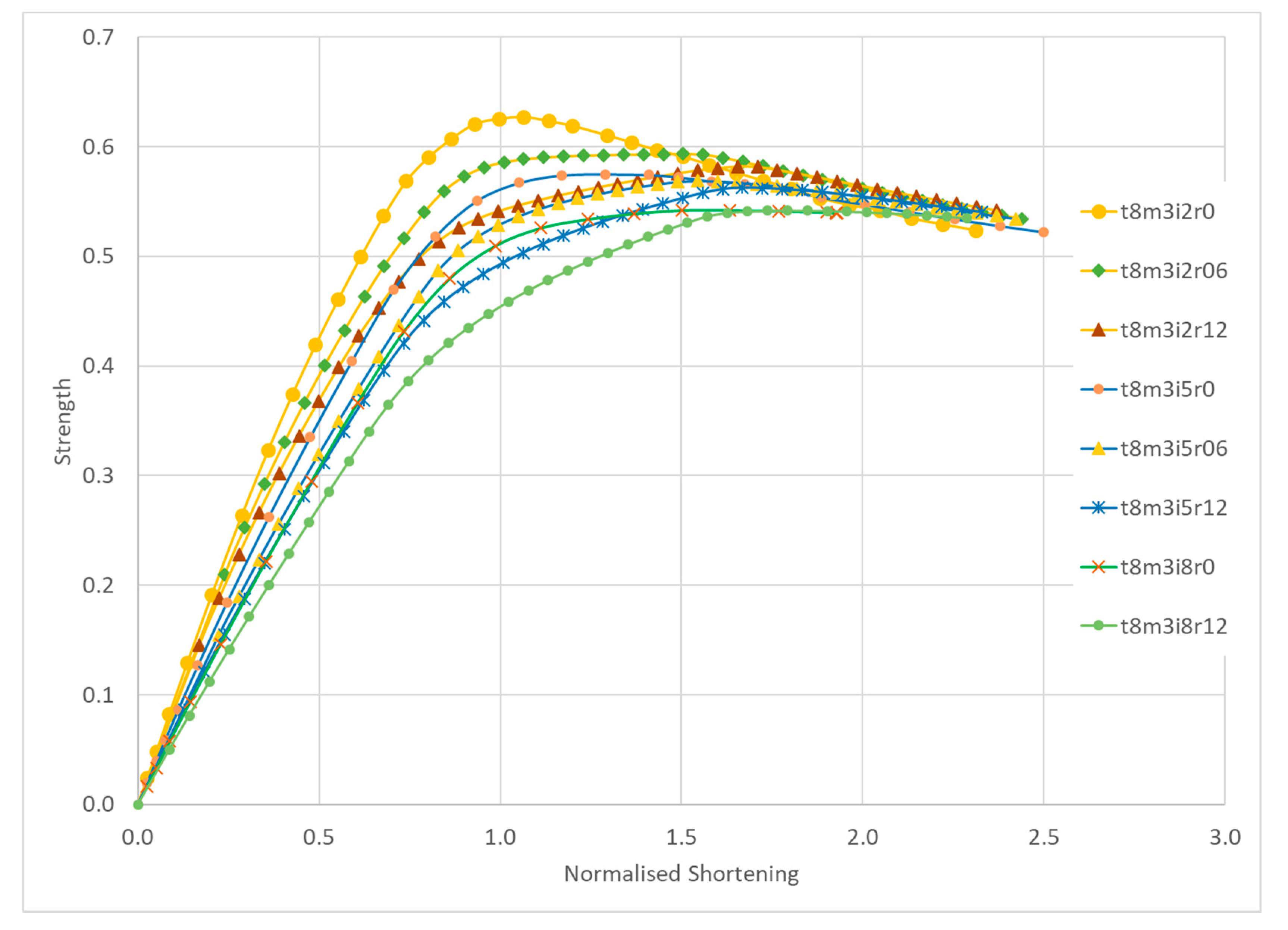
3.4. Very Slender Plates

The plates in this group have a slenderness, β, of 2.54 (b/t = 75). The reference value for the initial imperfections of these plates, w_i, is 5.14 mm according to Equation (9) and a w_i/t ratio of 0.643. Three levels of imperfections, w_i = 2, 5 and 6 mm and residual stresses of 0, 0.06 and 0.12 σ_y are considered. The LSC’s of this group of plates are shown in Figure 12.

Table 4. Summary of data and main results for plates with a = 1.5 m, b = 0.6 m and t = 8 mm.

Identification	Mode i	wi (mm)	wi/t	η	Ultimate Stress	Ultimate Strain	Residual Stress %
t8m3i2r0	3	2	0.25	0	0.627	1.063	0.00
t8m3i2r07	3	2	0.25	2	0.593	1.505	0.06
t8m3i2r15	3	2	0.25	4	0.582	1.654	0.12
t8m3i5r0	3	5	0.63	0	0.575	1.289	0.00
t8m3i5r07	3	5	0.63	2	0.569	1.544	0.06
t8m3i5r15	3	5	0.63	4	0.563	1.668	0.12
t8m3i6r0	3	8	1.00	0	0.542	1.633	0.00
t8m3i6r07	3	8	1.00	4	0.542	1.792	0.12

presents the main results of the ultimate strength and the corresponding normalized shortening for the different cases.

Since the slenderness of this group is very high the ultimate strength of the plates is small but does not degrade much with increase in imperfections and residual stresses, as presented in Figure 13. In fact, the ultimate strength of plates with residual stresses is almost insensitive to imperfections as confirmed by the very low coefficient 0.044 in Equation (18), but the pre-collapse behavior is rather dissimilar for each of them in terms of structural modulus and softening until collapse, Figure 12.

The ultimate normalized shortening of residual stress-free plates tends to be greater than in previous groups and the one for plates with residual stresses is much smaller than the values between 1.8 and 2 found previously. This is the result of the very low level of loading carrying capacity of these very slender plates.

The degradation of the ultimate strength due to increase on amplitude of imperfections is the smallest of all groups of plates with critical mode considered in this study and the ultimate strength can be quantified as:

$${\varphi }_u\left(\beta =2.54;rs=0\%\right)=0.652-0.114\frac{w_i}{t}$$

(17)

The equation for the ultimate strength for plates with residual stress of 12% of the yield stress is given by:

$${\varphi }_u\left(\beta =2.54;rs=12\%\right)=0.587-0.044\frac{w_i}{t}$$

(18)

These results confirm the conclusion of Ueda et al. [33] that welding residual stresses reduce the buckling strength remarkably but have a little effect on the ultimate strength when the plate is thin.

4. Discussion

The present methodology proved to be very efficient on the structural analysis of plate elements with residual stresses. The method is only based on mechanical and thermal properties of the material and allows to obtain the analysis in short time of computation with high accuracy.

The results obtained show how the main parameters already indicated in Section 3 affect the load-shortening curves (LSC), the ultimate strength and the corresponding ultimate shortening. The results were partially analyzed for each group of plates and formulas were presented for the ultimate strength of imperfect plates with and without residual stresses. Three main aspects need deeper discussion:

• Effect of slenderness on ultimate strength and correlation with imperfections and residual stresses;
• Dependency of structural tangent modulus from initial conditions of plate, i.e., geometry, imperfections and residual stresses;
• Effect of residual stresses in the LSC’s.

The analysis performed for each group of plates indicates that the main parameters may affect the ultimate strength largely, in some cases by more than 20%. Two modes of imperfections (m = 1, 3) were considered in some groups of plates to demonstrate this variation. For the stocky plates (t = 20 mm) without residual stresses, one may find a difference of 2% or 20% depending on the amplitude of imperfections, 2 mm and 10 mm respectively.

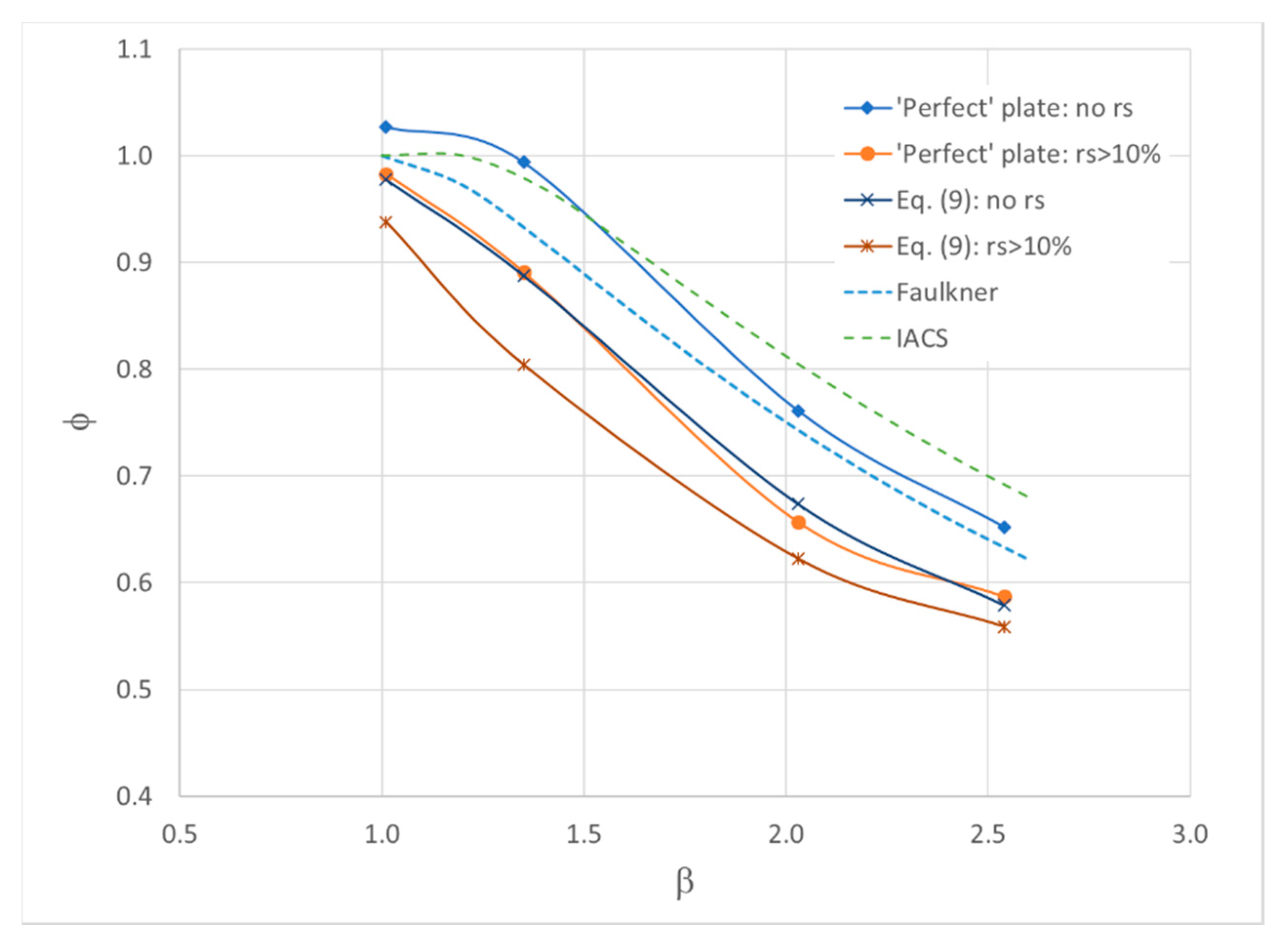
4.1. Effect of Slenderness on Ultimate Strength and Correlation with Imperfections and Residual Stresses

The dependency of ultimate strength on slenderness may be obtained by treating the strength equations for each group in integrated manner. Each equation has a constant term that represents the strength of virtual ‘perfect’ plate in terms of imperfections and a term related to the degradation of strength due to amplitude of imperfections. Collecting such information, one may present the relationship between strength and slenderness, as plotted on Figure 14, where some usual strength formulations are also plotted for comparison.

The curves for the influence of imperfections (Equation (9): no rs) and for effect of residual stresses alone (‘Perfect plate: rs > 10%) are very close, which means that the effect of imperfections or residual stresses individually are of the same order in comparison to virtual ‘perfect’ plate (‘Perfect’ plate: no rs). Nevertheless, the corresponding ultimate shortening and the LSC for each case are completely different.

The comparison of the plates with average imperfections but no residual stresses (Equation (9): no rs) or with residual stresses (Equation (9): rs > 10%) allows to conclude that the degradation of strength due to residual stresses is more marked in intermediate plates in the range of slenderness from 1.2 to 1.7. Thin plates are poorly affected by residual stresses as mentioned previously.

Curve ‘Equation (9): rs > 10%’ is representative of real welded plate and may be given by:

$${\varphi }_u\left(\beta ;\frac{w_i}{t}=0.1{\beta }^2;rs>10\%\right)=0.309+\frac{0.645}{\beta }$$

(19)

One aspect of concern in relation to structural codes is that all curves with exception for the ‘‘Perfect’ plate: no rs’ curve, are well below the Faulkner and IACS formulation. This may be result of boundary conditions of the tests that are the database for such formulations, inducing fixed conditions or some degree of rotational restraining.

4.2. Dependency of Structural Tangent Modulus from Initial Conditions

The comparison of initial stage of LSC for different initial imperfections with the same slenderness leads to the conclusion that plates present different structural tangent modulus in elastic range, where structural tangent modulus is the slope of the LSC, δσ/δε. This means that the plate suffers a loose of effectiveness in early stages of loading due to out-of-plane of initial imperfections. With the increase in the compressive loading, the out-of-plane geometry of plate increases, generating additional loss in effectiveness. The effectiveness depends not only on the level of imperfections but also on the slenderness of the plate. 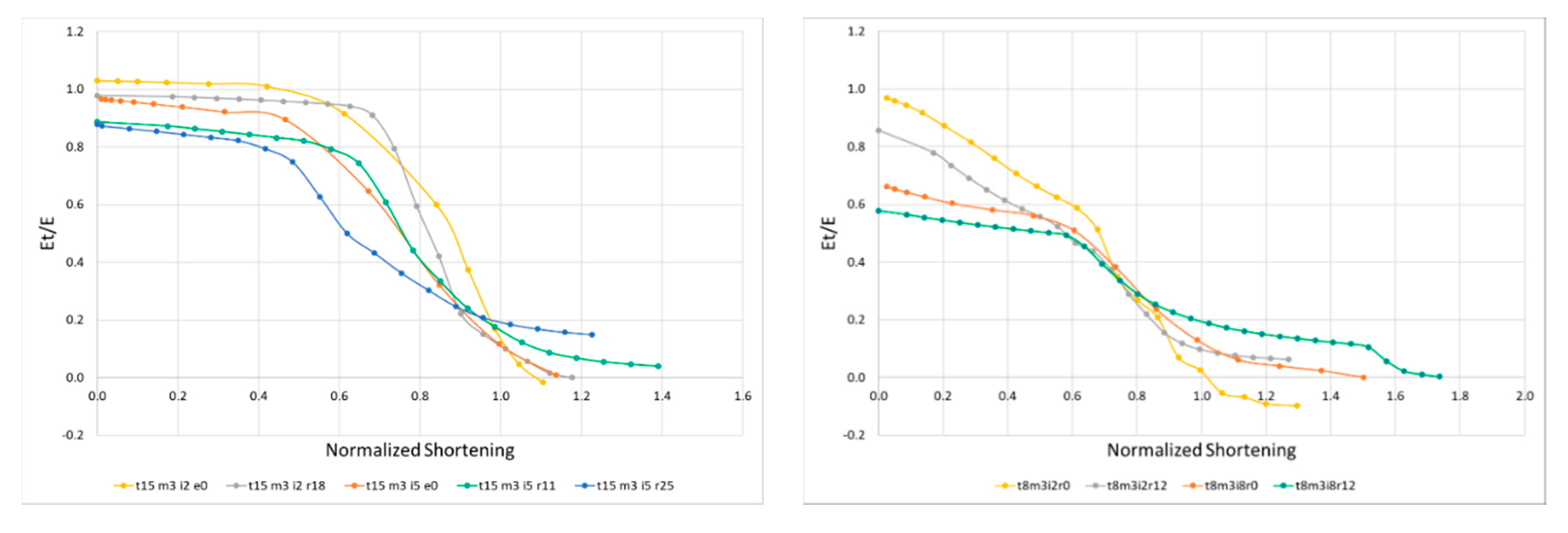Figure 15 plots the normalized tangent modulus of the plate for different thicknesses, t = 15 mm at left and t = 8 mm at right, for different amplitudes of initial imperfections and residual stresses.

The reduction in effectiveness at early stage of load is larger in slenderer plates and increases with w_i in both cases, as seen by comparison of yellow and red curves in both graphics. The presence of residual stresses represents a further reduction on initial effectiveness measured as E_t/E. The total reduction can be very high, representing a great softening of the structural element in elastic range.

This aspect requires further investigation in future research because it may have consequences on the response of 3-D structures, like the hull girder, under longitudinal bending.

4.3. Effect of Residual Stresses in the LSC’s

The results obtained for imperfect plates with residual stresses confirms the hypotheses adopted by Gordo and Guedes Soares [4] to generate predictive LSC’s for unstiffened and stiffened plates, ${\varphi }_{pl}\left(\epsilon \right)$. In such work, LSC are obtained by the product of the effective width of the plate without residual stresses at each level of loading, ${\varphi }_{ef}\left(\epsilon \right)$, and a modified material behavior that includes the effect of the tensile strips in HAZ, ${\varphi }_{mat+rs}\left(\epsilon \right)$, reading as:

$${\varphi }_{pl}\left(\epsilon \right)={\varphi }_{ef}\left(\epsilon \right)·{\varphi }_{mat+rs}\left(\epsilon \right)$$

(20)

Figure 16 shows ${\varphi }_{mat+rs}\left(\epsilon \right)$ for compression and tensile loading. This response is very well reproduced by the stocky plates presented in this study, Figure 6, where the effectiveness ${\varphi }_{ef}\left(\epsilon \right)$ is close to 1. In all other groups of plates, the behavior reproduced by the red dot line is present, but curves in the range of strain affected by residual stresses are not totally straight due to the reduction on ${\varphi }_{ef}\left(\epsilon \right)$.

Furthermore, ${\varphi }_{ef}\left(\epsilon \right)$ proposed in [4] was based on Faulkner’s formulation. For the prediction of LSC of unstiffened plates with average imperfections in critical mode and constrained edges, curves from Figure 14 should be used, in particular the curve ‘Equation (9): no rs’ representative of plates with average imperfections and no residual stresses.

5. Conclusions

A methodology to evaluate the performance of welded structural element was presented and shows to be efficient and reliable in the study of unstiffened plate elements under compression.

The parameters used in this study, slenderness, residual stresses, mode and amplitude initial imperfections, prove to be of high importance in the prediction of the ultimate strength but also in the response prior to collapse. The variation in ultimate strength of plates due to the change of magnitude of one parameter alone may reach high values.

Residual stresses affect the pre-collapse behavior of the plates very much, but the ultimate strength tends to be the same, keeping other parameters constant. The corresponding ultimate strain is much higher than in the case of residual stresses free plate, which means that one has a softer response with increase in residual stresses level.

Both residual stresses and initial imperfections affect the initial slope of LSC, structural tangent modulus, and this may affect the performance of 3-D structures, so it should be considered in the future.

Future application of this methodology involves the study of the structural behavior of welded stiffened plates and 3-D structures, considering different loading conditions.