Article

Near-Surface Transport Properties and Lagrangian Statistics during Two Contrasting Years in the Adriatic Sea

1
Ifremer, Department of Coastal Environment Dynamics (DYNECO), 29280 Plouzané, France
2
National Institute of Oceanography and Experimental Geophysics (OGS), Borgo Grotta Gigante 42/c, 34010 Sgonico Trieste, Italy
J. Mar. Sci. Eng. 2020, 8(9), 681; https://doi.org/10.3390/jmse8090681
Submission received: 4 August 2020 / Revised: 30 August 2020 / Accepted: 2 September 2020 / Published: 4 September 2020
(This article belongs to the Section Physical Oceanography)

Abstract

:
This paper describes the near-surface transport properties and Lagrangian statistics in the Adriatic semi-enclosed basin using synthetic drifters. Lagrangian transport models were used to simulate synthetic trajectories from the mean flow fields obtained by the Massachusetts Institute of Technology general circulation model (MITgcm), implemented in the Adriatic from October 2006 until December 2008. In particular, the surface circulation properties in two contrasting years (2007 had a mild winter and cold fall, while 2008 had a normal winter and hot summer) are compared here. In addition, the Lagrangian statistics for the entire Adriatic Basin after removing the Eulerian mean circulation for numerical particles were calculated. The results indicate that the numerical particles were slower in this simulation when compared with the real drifters. This is because of the reduced energetic flow field generated by the MIT general circulation model during the selected years. The numerical results showed that the balanced effects of the wind-driven recirculation in the northernmost area(which would be a sea response to the Bora wind field) and the Po River discharge cause the residence times to be similar during the two selected years (182 and 185 days in 2007 and 2008, respectively). Furthermore, the mean angular momentum, diffusivity, and Lagrangian velocity covariance values are smaller than in the real drifter observations, while the maximum Lagrangian integral time scale is the same.

1. Introduction

1.1. Overview of the Application of Lagrangian Methods in the Adriatic Sea

Over the last 40 years, the dynamical characteristics of oceanic flows have been widely analyzed using Lagrangian approaches. Lagrangian particles are used to study the transport properties of flows, such as the transit and residence times of drifters, because they move closely with the water parcels, especially in large and mesoscale ranges. Additionally, Lagrangian methods are powerful tools used to display the mixing activities of flow currents by applying and developing mathematical theories (e.g., finite size Lyapunov exponents (FSLE) and finite time Lyapunov exponents (FTLE)).
Falco et al. [1] have discussed the surface transport properties in the Adriatic Sea using a drifter dataset ranging from December 1994 to March 1996. In their study, a Lagrangian transport model for simulation of numerical particles was employed with parameters derived from the drifter data. As their results showed, the model was able to reproduce reality with good approximation, except for specific advective conditions in the summer season during September. Falco et al. [1] mentioned that the residence time values for real drifters in the Adriatic are between 70 and 90 days because of the finite lifetime of the drifters, while numerical particles simulated by the model suggested a correct value of 200 days.
In another study by [2], the statistics of transit and residence times in the Adriatic Sea surface were estimated from drifter data and Lagrangian numerical simulations. They found that the results obtained for the drifters were generally underestimated given their short operating lifetimes (half-life of ~40 days) compared to the transit and residence times, so they implemented numerical particles whose trajectories were integrated over a longer time period (750 days) with a statistical advection–dispersion model of the Adriatic surface circulation. They indicated that the maximum transit time to exit the Adriatic Sea is about 216–260 days for the particles located at the northern end of the Adriatic, while a particle entering on the eastern side of the Otranto Channel will exit from the basin after 170–185 days. Moreover, they calculated 150–168 days as the residence time of numerical particles in the Adriatic Basin.
The effect of wind forcing on the Western Adriatic Current (WAC) was studied by [3]. Their results showed that the Adriatic promontories, in the absence of wind, induce instabilities in the boundary currents, while the persistent downwelling-favorable northwesterly winds thicken and narrow the flow current; in this case, the transport is generally southward, where instabilities measuring ~10 km in size ultimately vanish after developing because of the lack of across-shore space to grow. On the contrary, the upwelling-favorable southeasterly winds allow the instabilities to grow into mesoscale features (~35 km), considering that transport decreases and changes direction.
In another study by [4], the spatial structures of the surface currents at meso- to seasonal scales were estimated from more than 200 satellite-tracked drifters during 1990–1999 in terms of Eulerian and Lagrangian statistics. Some of these data have been used in this paper for comparison with the numerical simulations.
Following the same subject, Maurizi et al. [5] examined the properties of mesoscale Lagrangian turbulence in the Adriatic Sea from drifter datasets in 1990–1999 based on the influences of inhomogeneity and non-stationary. They detected three main regions of the Adriatic where the velocity statistics are approximately homogeneous: the two boundary currents, the West and East Adriatic Currents (WAC and EAC), and the southern central gyre. In the center of the Southern Adriatic, the results show symmetric probability density functions of velocity with exponential autocorrelations, while the boundary regions are instead significantly asymmetric, with skewness indicating preferential events in the direction of the mean flow.
The aim of the work by [6] was to detect Lagrangian transport barriers in the Gulf of Trieste by means of the Lyapunov exponent approach. They calculated Lagrangian coherent structures (LCSs) using 2D surface velocity fields measured by the coastal radars of the Tracking Oil Spills and Coastal Awareness Network (TOSCA) EU research project. They showed that transport can be studied through the concurrent use of FTLEs, FSLEs, and Lagrangian coherent structures (LCSs). A direct comparison of FTLEs and FSLEs by evaluating their correlation indicated that there is agreement between them. Their results showed that both FTLE and FSLE fields are able to locate the same pattern of Lagrangian structures in real geophysical flows characterized by large Reynolds numbers. They emphasized that Lyapunov exponents (FTLE and FSLE) are valuable tools for evaluating the main directions along which transport phenomena are likely to occur.
Carlson et al. [7] used surface drifters and virtual particles to investigate transport between seven coastal regions in the central and southern Adriatic Sea to estimate the degree to which these regions function as a network. They mentioned that southeasterly Sirocco winds can drive eastward cross-Adriatic transport from the Italian coast near the Gargano promontory to the Dalmatian Islands in Croatia, while disrupting alongshore transport on the west coast. Moreover, their results displayed that in the central Italian regions, there are strong connections from north to south, likely realized by alongshore transport in the WAC.
De Dominicis et al. [8] quantified the sub-grid scale diffusion of the Lagrangian models written in terms of horizontal eddy diffusivity. They used a large database of drifters released in different regions of the Mediterranean Sea; the Lagrangian sub-grid-scale diffusion was computed by considering different regimes when averaging statistical quantities. Moreover, they simulated the real drifters using a trajectory model forced by Ocean General Circulation Model (OGCM) currents to investigate how the Lagrangian properties are reproduced by the simulated trajectories.
Other applications of the Lagrangian technique have been extensively discussed by [9,10,11,12,13,14,15,16].

1.2. Description of the Study Area

The Adriatic Sea is a challenging and interesting semi-enclosed basin for the study of dynamical characteristics by applying Lagrangian methods. The mean Adriatic general circulation in the surface layers is characterized by a large cyclonic gyre, in which seawater flows northwards along the Balkan coast (the EAC) and southwards along the Italian coast (the WAC). Recirculation cells are present at the latitude of the Palagruza Sill; the Middle Adriatic Pit near Split, Croatia; and south of the Istrian Peninsula [17,18,19,20,21,22,23].
The influence of topography on the current field and the strong seasonality of currents near the coast, which is stronger in summer (fall) along the Italian coast (eastern side), was partially confirmed by [4]. He has also proved that the WAC within 10 km of the Italian coastline is almost the same during the other seasons, while the EAC is stronger in fall. In addition, summer and fall are the most energetic seasons [4,23]. In the Adriatic Sea during winter and spring, the maximum velocities are located near the coast [4] and the mean kinetic energy is maximal in fall and winter in the central and southern sub-basins. In the southern WAC, the speeds are greater and the velocities measured during spring are lower compared to the other seasons. The Adriatic surface circulation reveals a strong seasonality, which can be explained in terms of wind-forcing variability [17]. With Bora wind, the across-basin recirculating currents and the WAC are intensified, while in the Sirocco regime northward flow without recirculation dominates in the eastern part of the basin [23]. Moreover, a strong dependence between the WAC and the Po River runoff was observed. The river runoff influenced not only the currents, with an increase of speed during high discharge rates, but also strengthened the recirculation around the Middle Adriatic Pit [23].
In this study, the dynamical characteristics of the Adriatic Sea were focused on by using Lagrangian methods. The aim of the work was to investigate the effects of surface currents on the movement of numerical particles deployed on the surface. Moreover, the influence of river discharges and wind flow fields on transit and residence times of numerical drifters was examined during selected periods.
In the second part of the study, the following questions were answered: How did particles disperse away due to the fluctuating velocities during 2007 and 2008 compared with real data? How long does the memory of the numerical particles last? I tackled these issues through the calculation of Lagrangian integral scales and eddy diffusivities.
This study indicates that Lagrangian analysis is a powerful way to analyze the output of ocean circulation models and other ocean velocity data, considering that the Lagrangian approach plays an important role in many practical areas, including water quality management, planning for pollutant discharge, sediment tracking near river or stream mouths, and prevention of rivermouth clogging. Other applications include management of water recycling and discharge within ports, management of marine ecosystem protection activities, and the provision of detailed predictions for intervention scenarios in exceptional events such as oil spills. On the other hand, based on the definition of turbulent flow, the fundamental basis of the mixing processes in the ocean is related to the Eulerian flow field, but since mass transport is a Lagrangian phenomenon (which can be affected by meso- and sub-mesoscale parameters associated with coherent structures), it is necessary to use Lagrangian tools for dispersion modeling.
As mentioned above, this paper provides a comprehensive description of the dynamic parameters of the Adriatic Sea circulation using Lagrangian methods. The present work, compared to previous studies, highlights the effects of seasonal and interannual variability on the movement and transport of numerical particles for specific years because of different climatological conditions. In other words, this study gives a clear picture of the evaluation of the environmental effects on particle displacement.
The paper is organized as follows to address the above issues. Section 2 provides information on the Adriatic Oceanic General Circulation Model (OGCM) and the Lagrangian models used to compute the numerical experiments. The results and discussion are presented in Section 3, and the summary and conclusions are given in Section 4.

2. Data and Methods

2.1. The Adriatic OGCM

The hydrodynamic model used in this study was generated with the state-of-the-art (Massachusetts Institute of Technology general circulation model (MITgcm; [24]). The MITgcm is based on a three-dimensional, finite-volume spatial grid with z-levels. The model solves the non-hydrostatic Navier–Stokes equations, adopting an implicit linear formulation of the free surface. More information about the code can be found in the documentation available at: http://mitgcm.org/public/r2_manual/latest/online_documents/manual.pdf.
The model in this study covers the whole Adriatic Sea, with a horizontal resolution of 1/32° (approximately 3.4 km × 2.4 km). Simulations were performed for the period ranging from October 2006 to December 2008. The time step for the integrations was 300 s, while the time required to model one year was 3.6 days. This model had 51 unequally spaced z-levels characterized by vertical resolution, which decrease with depth (a resolution of 1.5 m at the surface and 50 m in the bottom layer corresponding to the grid spacing in the z coordinate). The bathymetry was obtained by interpolating a dataset collected in the framework of the ADRIA02 project. The initial conditions for temperature, salinity, and the zonal and meridional components of velocity were derived from the 1/16° operational analysis of the Mediterranean Sea (Mediterranean ocean forecasting system model—MFS; [25]). River runoffs provided from 17 major rivers along the Albanian, Croatian, and Italian coasts were included in the lateral boundary conditions. The freshwater discharge of the major rivers was extensively explained by [26,27]. The surface forcing was obtained by interpolating the atmospheric heat and mass fluxes computed by the MFS model and the high-resolution wind fields provided by the ETA006 (courtesy of CREST S.r.l.—Physics and Engineering for Marine Environment) and ALADIN (data provided by the Research and Atmospheric Modeling Department of the Meteorological and Hydrological Service of Croatia) models. The model neglects tides, indicating that tidally induced residual currents in the Adriatic are generally supposed to be negligible for large parts of the basin. Further details on the hydrodynamic implementation of the present simulation, including numerical methods, closure schemes, turbulent coefficients, and model validation, are reported by [27,28].

2.2. The Lagrangian Model

Each numerical particle trajectory was obtained by interpolating the U (velocity fields) between grid points (bilinear interpolation in space and linear interpolation in time) and integrating the following equation:
d x = ( U ) d t
Using a fourth-order Runge–Kutta scheme, the time step dt was taken as 1 h. Since the flow fields obtained by the MITgcm in this study are daily averages, linear interpolation in time was applied. A reflection wall condition was also adopted along coastlines; if the particles were to reach the coastline, they would come back again inside the basin.
Overall, 1080 particles were integrated over one-year periods (2007 and 2008). The resolution of the grid points in both zonal and meridional directions was 0.03125°. The choice of 1080 numerical particles was quite arbitrary. The particles were deployed uniformly inside the basin at the same time. The results were analyzed in detail in three sections along the Italian coastline, in the Conero and Gargano promontories, and in the Strait of Otranto.
The residence time is defined as the average time spent by a tracer particle in the basin. The normalized population in the basin, C(t), and its residence time, T, in the Lagrangian framework are [2]:
C ( t ) = N ( t ) N ( 0 )
T = lim T * t
T * = t N ( t ) N ( 0 ) + i = 1 N e ( t ) t e i N ( 0 )
where N(0) is the number of tracer particles initially deployed in the basin, N(t) is the number of particles at time t, Ne is the number of particles that have already escaped the basin at time t, and tei is the escape time of the ith particle.

2.3. Calculation of Lagrangian Statistics

From a theoretical point of view, the calculation of Eulerian statistics should be done by an ensemble of many data realizations obtained in the Adriatic Sea [1]. Furthermore, Lagrangian velocity statistics are computed over an ensemble of selected particles. In this case, each observation in the domain was assumed to be a deployment position from which the particle is followed. Lagrangian statistics are calculated for positive and negative time lags [29]. In order to compute the Lagrangian statistics for the entire Adriatic Basin in 2007 and 2008, first the deterministic Eulerian mean flow was subtracted from the individual particle velocities. The mean Eulerian velocity field was interpolated at the particle locations using bilinear interpolation. The values of Lagrangian velocity covariance, diffusivity, and Lagrangian time and space scales were computed. The symbol L is specified to show the averaging over time and space computed at time lag τ before or after the particles are located in a given domain. Therefore, the Lagrangian mean velocity is u i L ( τ ) . It should be noted that the averaging method is similar to [4].
The Lagrangian velocity covariance matrix is given by (here, i (X) and j (Y) represent along- and across-basin directions respectively as shown in Figure 1a):
p i j ( τ ) = u i ( 0 ) u j ( τ ) L
where x i ( τ ) and u i = u i u i L ( i = 1 , 2 ) are the particle position and residual Lagrangian velocity components, respectively.
For the sake of completeness, other well-known statistical quantities that will be used to characterize the Lagrangian motion will be introduced.
The diffusivity matrix [29] is, therefore, defined as:
K i j ( τ ) = u i ( 0 ) ( x j ( 0 ) x j ( τ ) ) L
The Lagrangian covariance is related to the diffusivity matrix by:
K i j ( τ ) = τ 0 p i j ( t ) d t
The Lagrangian integral time and space scales are defined as:
T 1 i ( τ ) = K i j ( τ ) / p i j ( 0 )
L 1 i ( τ ) = K i j ( τ ) / p i j ( 0 )
Additionally, the kinetic energy (per unit mass) of the mean flow and mean eddy kinetic energy (MKE and EKE) are given by (based on the Eulerian statistics):
M K E = 1 / 2 ( < u 1 > E 2 + < u 2 > E 2 )
E K E = 1 / 2 ( < u 1 u 1 > E 2 + < u 2 u 2 > E 2 )

3. Results and Discussion

3.1. Adriatic Mean Circulation Properties Obtained by Lagrangian Velocity Fields

The first part of the results presents the Adriatic mean surface circulations in 2007 and 2008 as derived from synthetic trajectories (Figure 1). Three main circulation cells were obtained from the particle velocities in the Adriatic Sea.
In general, the mean flow maps (Figure 1) generated by synthetic trajectories in 2007 and 2008 confirm most of the results obtained previously from drifter observations [2] and hydrographic data.
As the flow maps (Figure 1) during both years clearly show, recirculation cells are found in correspondence with the Palagruza Sill, the Middle Adriatic Pit near Split, and south of the Istrian Peninsula [4,30,31]. The energetic (prevailing) currents along the eastern and western flanks of the Adriatic were detected in the mentioned periods, which indicate the high energetic flow rates along the EAC and the Italian coastline, although during 2008 this was more visible. In the north end of the Adriatic, as numerical results show, the mean flow in 2008 was more intense and presented higher speeds compared to 2007, considering that it generates the fourth isolated cyclonic gyre north of Po River, which has an important role in the movement and transit of numerical particles located in this area. The aforementioned semicircular anticlockwise flow developed under the influence of seasonal windstress curl.
On the other side of the northern Adriatic, an anticyclonic pattern, which is located off of Istria between a cyclonic structure in the northern basin up to the Po River delta and the branch of the EAC recirculation (Ursella et al., 2006), did not appear in the mean circulation maps generated by the model in either year (Figure 1).
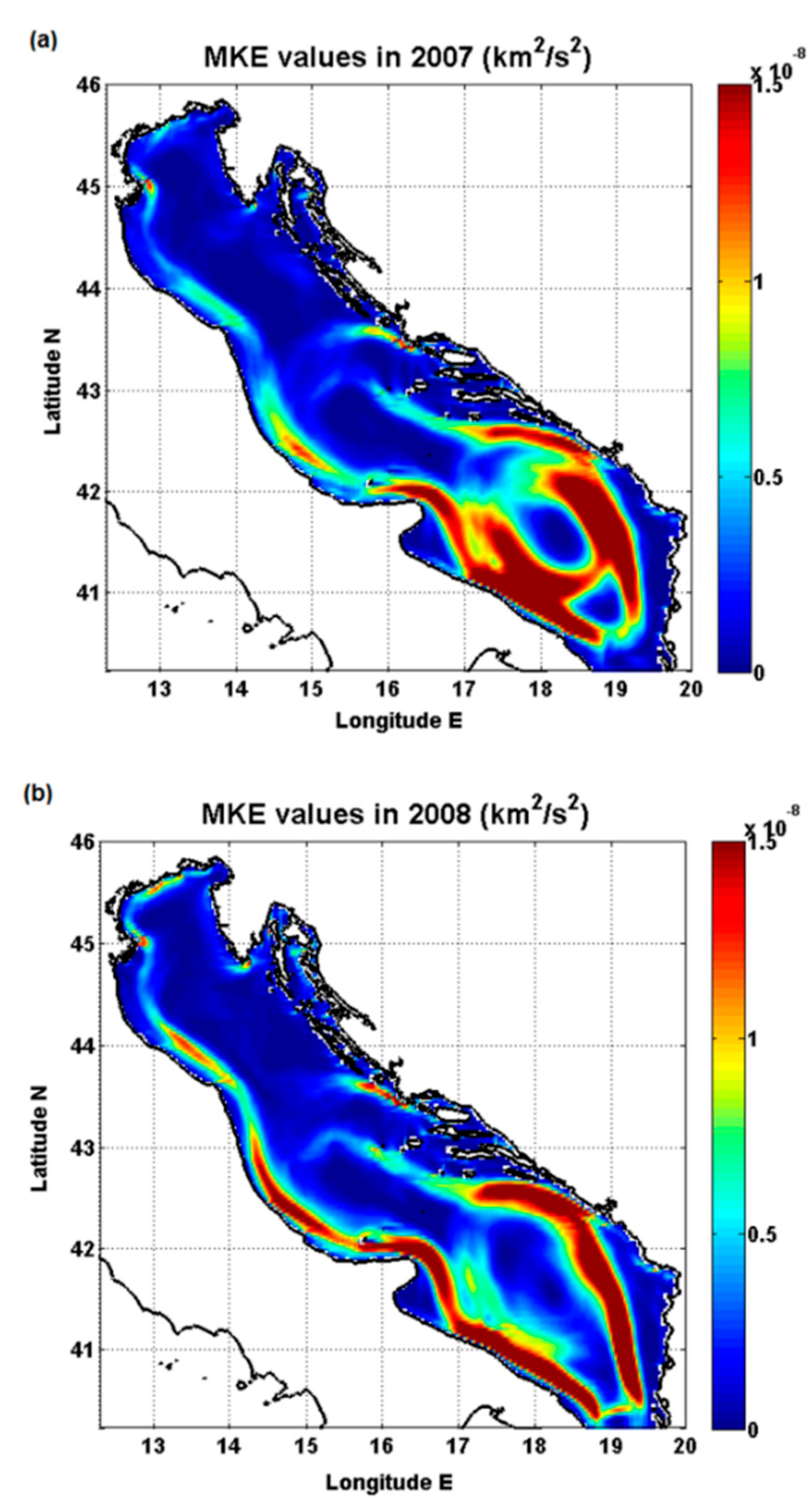
The flow fields obtained by Lagrangian data indicate that the central Adriatic had the same conditions in both years, which was mainly affected by the EAC and WAC; however; the return flows from the eastern flank of the Adriatic in 2008 had higher values of MKE (Figure 1 and Figure 2). This property of the flow current helps numerical particles to exit more quickly from the basin. The dispersion process of synthetic trajectories in the Northern Adriatic takes a long time because of the stable and less energetic flow fields in this area; moreover, the turbulent velocity fluctuations are negligible.
The Southern Adriatic Pit (SAP) in both years has the highest velocity values, since it is under considerable influence fromseasonally positive wind curl (Sirocco-wind) and intensive inlet flows from the Ionian Sea. This characteristic leads to high values of mixing activities in the south of the Adriatic, which creates small and energetic vortices thattransfer energy and momentum between different parts of the basin (Figure 1 and Figure 3).
Additionally, Lagrangian mean flow fields (Figure 1) highlight the basin-wide cyclonic circulation, particularly for the EAC (northward currents along the eastern side) and a fast return flow along the Italian coast on the western side (WAC), where sub-basin recirculation cells in the central and southern Adriatic Sea are involved in this pattern.

3.2. Transit and Residence Times of Numerical Particles during Two Contrasted Years (2007–2008)

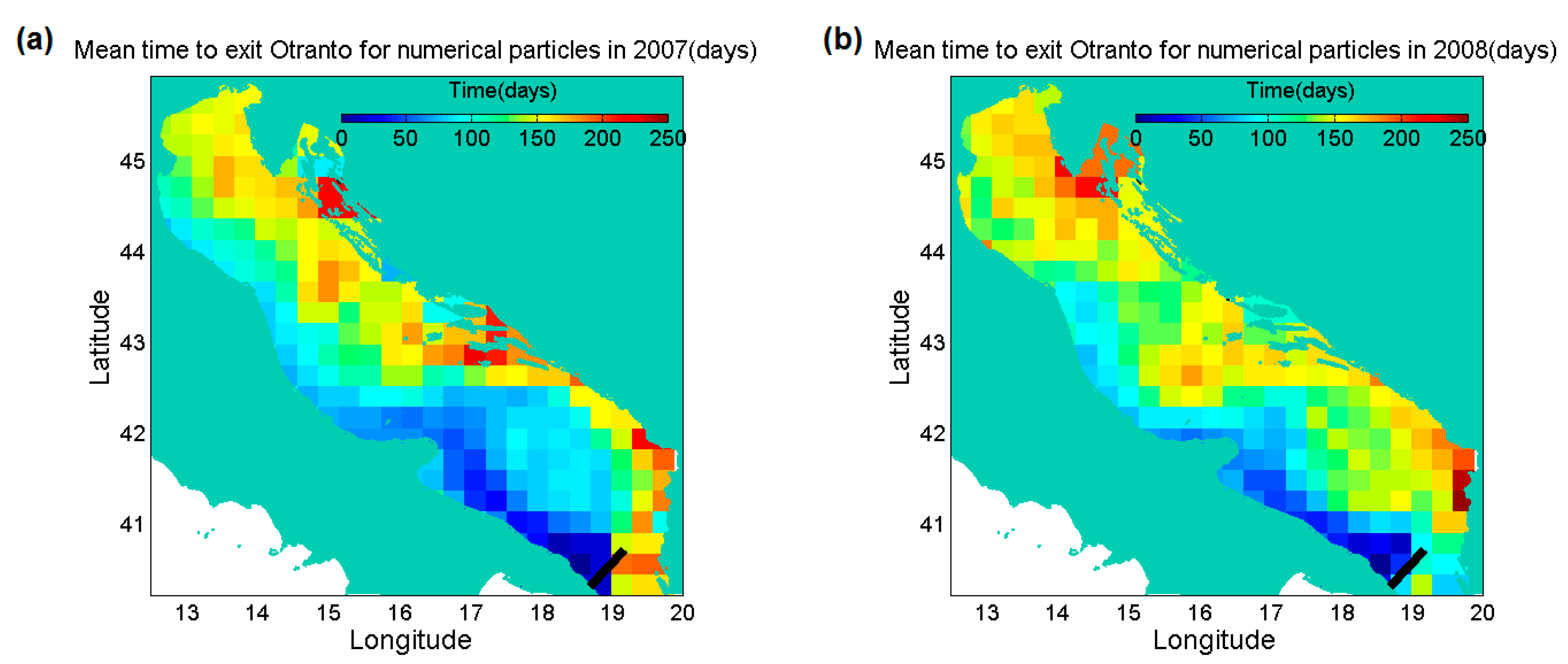
In order to analyze the transport pattern of the numerical particles affected by mean flow fields, values for thetransit times (the time that is needed for a drifter to move inside the basin) of synthetic drifters crossing the Strait of Otranto were calculated. As Figure 4 shows, the highest transit time values are related to the eastern Adriatic Sea close to the Albanian coastline and in front of the Istria Peninsula. This means that numerical particles located on the eastern flank of the Adriatic are influenced by the entrance flow from the Ionian Sea and that they stay for a longer period in the basin, increasing the mean residence timevalues. On the contrary, the effects of the Po River runoff are significantly visible along the Italian coast, given that this parameter (Po River discharge) reduces the transport times of the numerical particles in the WAC (Figure 4, Figure 5 and Figure 6).
Figure 5 shows that the highest values of the Po River discharge (these data are courtesy of Dr. Alessandro Allodi—Regione Emilia Romagna ARPA—SIM, Area Idrologia—PARMA) occurred in June, November, and December 2008. On the other hand, the lowest river discharge values were obtained in July and August 2007. Po River discharge during 2007 shows the lowest values compared to the other examined year. In addition, the monthly average values of the Po River discharge during the specified years (2006–2011) are represented in Figure 6. River discharge gradually increased from January to May and June and then decreased significantly during July and August, while in winter (November and December) the Po River discharge occurred at a similar rate as in May and June.
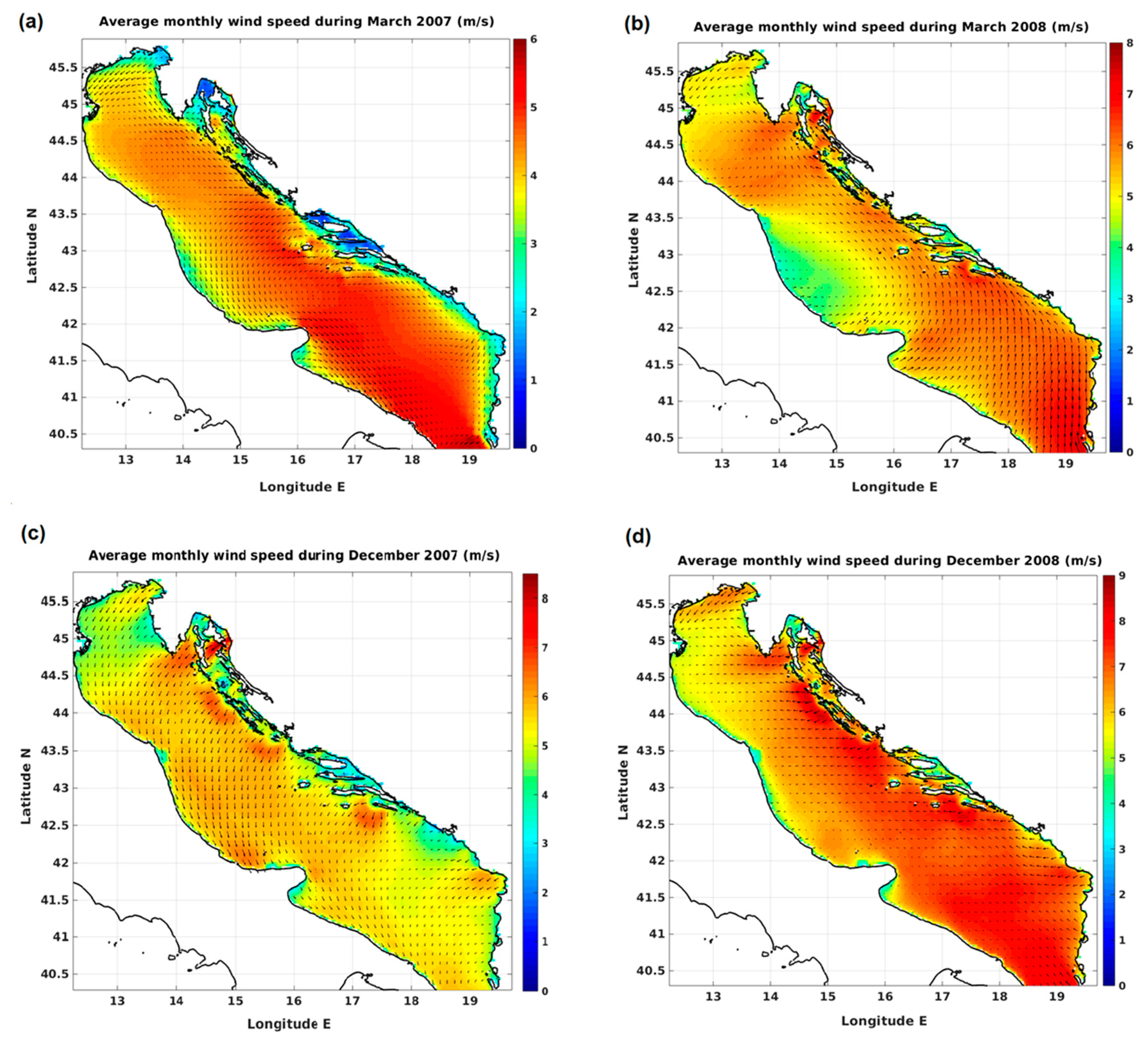
In the Northern Adriatic, the effect of the Bora wind as a negative wind curl is evident from the increase in transit time values for the numerical particles initially deployed in the Gulf of Trieste (this situation is more visible during 2008, Figure 4). Because of stable flow with lower mixing activities and low-velocity values, the transit times range between 125 and220 days in the Northern Adriatic during both years (Figure 3, Figure 4, and Figure 7).
In the center of the Adriatic Sea, the most frequent transit time values for numerical particles leaving the basin during 2008 were lower than in the previous year, while the mean transit time values were almost the same for both years. In addition, the numerical particles located off the Croatian coastline moved along the main Adriatic circulation cell to exit from the Otranto Channel. These numerical particles present high mixing activities in their pathways due to the influence of turbulence fluctuations, which increase the EKE and MKE values in this region (Figure 4).
In the Adriatic Sea, the SAP plays an important role in the transport process, particularly during the winter, due to the filamentary structures generated by the positive wind curl (Sirocco wind). Flow currents in the eastern part of the SAP force the numerical particles deployed in this area to move along the wide circulation cell inside the basin, so it takes a long time for the numerical drifters to leave the Adriatic, while the synthetic drifters located in the central and western parts of the SAP tend to cross the Otranto Channel immediately after entering the basin (this condition is more evident in 2007). On the other hand, in the core of the Southern Adriatic Sea during 2008, because of the existence of more energetic flow currents relative to 2007, high numbers of eddies were generated, increasing the mixing activity. However, they force the numerical particles to stay in the basin for an extended period by inducing the dispersion of numerical trajectories and increasing the flow instabilities.
Off the Istrian Peninsula, as a result of the effects of a small cyclonic circulation cell, longer transit times were detected relative to the whole basin, where the return flow from the EAC collides with the northern circulation cell. Generally, if the Adriatic Basin is divided into two sections, the eastern part of the basin is completely influenced by wind curls (positive or negative wind currents, Sirocco or Bora regimes), while in the western flank of the Adriatic, the Po River runoff plays a major role in transport time values (Figure 3, Figure 4, Figure 5, Figure 6 and Figure 7).
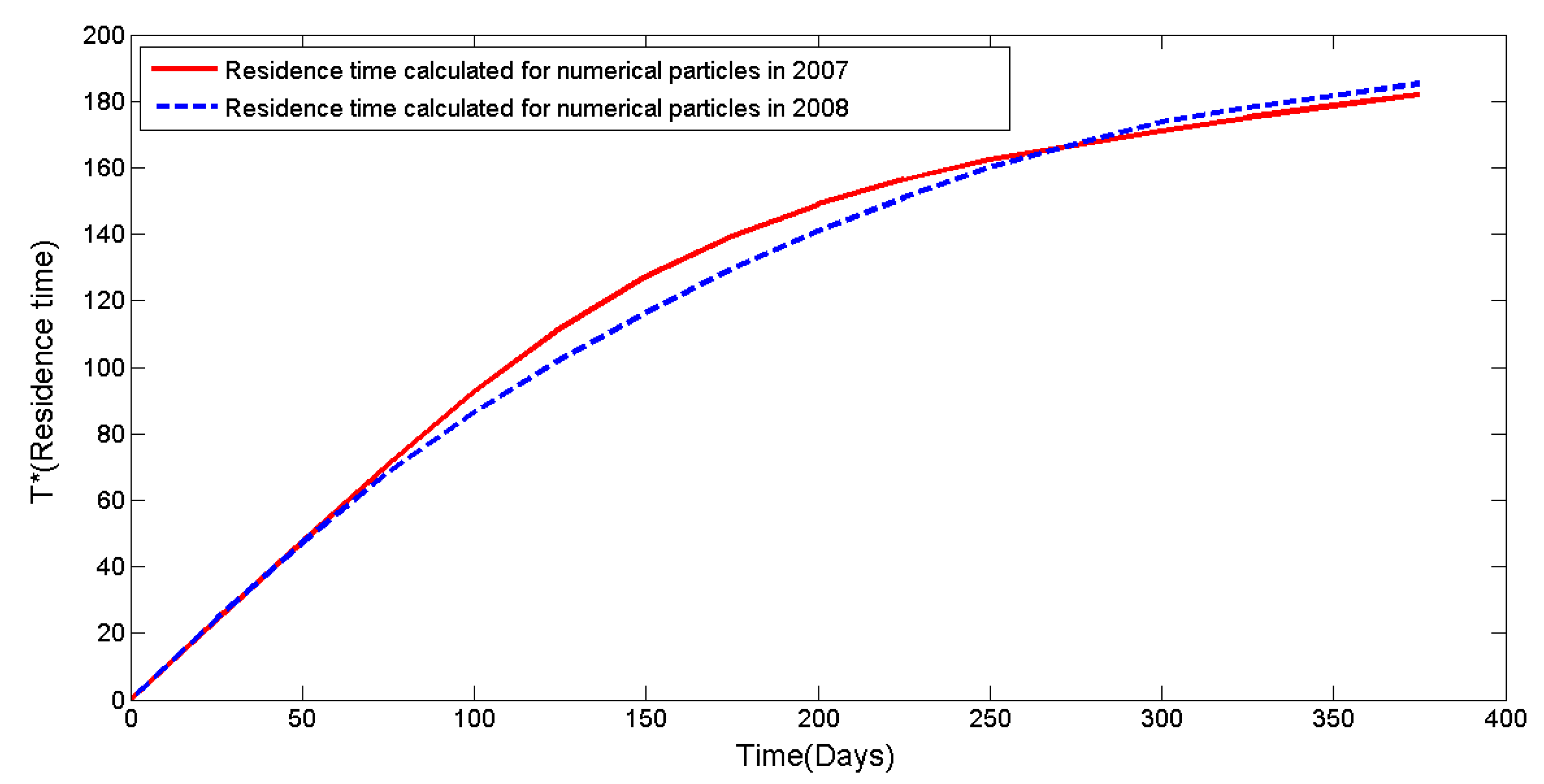
The residence time values (Figure 8) during both years were calculated in order to find the average lifetime for all numerical particles in the basin. The results clearly show negligible differences between the calculated residence times in 2007 and 2008; as a result of different weather conditions during each year (2007 had a mild winter and cold fall, while 2008 had a normal winter and hot summer), it was expected that the residence time values would be different, but the residence time value, T*, was 182~185 days after the maximum integration period (365 days) in both 2007 and 2008.
As discussed previously, wind forcing and river runoff are important parameters that affect the transit and residence times of numerical particles and drifters in the Adriatic Sea. The influence of the main wind currents (the Bora wind field, which dominates the Northern Adriatic, in particular the Gulf of Trieste, and the Sirocco regime, which generally affects the whole of the Adriatic Sea in fall and winter) on the transit time and residence time was examined in the preceding section; moreover, Figure 7 shows that most intense winds are from the northeastern sectors during wintertime and are more energetic (higher wind speed) in 2008 than in 2007. The wind-driven recirculation pattern up the Po River and off of Istria (as a sea response to the wind field and Bora events) creates a closed area in which numerical particles can remain for a longer period of time. My numerical simulations indicate that the residence time is longer during both years compared to the results obtained by [2].
In addition, the MKE fields (Figure 2) identify the areas with high turbulence instabilities in the basin and help to determine the relationships between transit and residence times of numerical particles with mixing properties. As MKE maps show, during both years due to the high inlet flows, in particular the Po River on the western side of the basin and the strong currents from the Ionian Sea on the eastern flank of the Adriatic Sea, the MKE values in these areas are higher compared to the other parts of the Adriatic. The transit times (and residence times) reach the lowest values at the edge of the Southern Adriatic and along the Italian coastlines (areas with high mixing activities). Numerical particles leave the Otranto Channel due to high-speed flow currents. These currents generate turbulent fluctuations by producing energetic transient eddies that facilitate the transport of numerical particles in the SAP (Figure 2 and Figure 4).
Table 1 presents a comparison between the previous studies and the current work, as results show that the real drifter transit time in the Adriatic is lower than found in both studied years. The results indicate that more accurate surface transit and residence times could be estimated using numerical simulations, and the approach used in this paper avoids the major problems that arise with real drifters. Real drifters produce defects in the estimation of residence or transit times because of their finite lifetime (mortality), while the scarcity of drifter data can introduce significant random and bias errors. The statistical results can also depend upon the specific deployment locations selected, while the numerical method applied in this paper improves and corrects this problem by allowing the use of many numerical particles in different parts of the basin. Transit times between entrance and exit through the Otranto Channel show that real drifters need about 83 days to transit the Adriatic, while numerical particles in 2007 and 2008 required 155 and 143 days, respectively, likely due to the long lifetimes of numerical particles and short lifetimes of real drifters. In addition, the fluctuation terms, which are normally added to the mean flow fields obtained by real drifter datasets, are not the same as for coherent turbulence (as in [2]), given that these turbulent terms are space-dependent and non-isotropic to the velocity variance, integral time, scale, and diffusivity (as it is known that these values vary significantly in the basin). In contrast, the flow fields obtained by OGCMs in high-resolution simulations do not need any improvements in their inclusion of turbulence parameters, as they contained enough turbulence to affect the movement of numerical particles. The sensitivities of the transit and residence time results to turbulence terms are clearly distinguished in the two case studies by [2] and in the current simulations, indicating that the parameters corresponding to the generation of turbulent transport (e.g., the random flight model used by [2]) have significant effects on transit time values (statistical results are summarized in Table 1). Another benefit of using numerical particles is that one can easily control the deployment array (e.g., ensure uniform deployment throughout the basin), the lifetime, and the number of particles. It should be added that the use of high-resolution hydrodynamical models costs much less than experimental observations such as drifter datasets, with the possibility of having the same mean flow and energy levels as the drifters. Moreover, hydrodynamical models allow for the integration of numerical particles in time-dependent velocity fields and the computation of Lagrangian statistics, such as the transit and residence times.
Moreover, two types of eddies were detected in the basin (based on FSLE and FTLE fields not shown in this paper); eddies and vortices were produced in the cores of circulation cells in the Southern, Middle, and Northern Adriatic Sea, which act as delay structures to force numerical particles to move more slowly within the basin. These types of eddies increase the mixing activities of numerical drifters by generating compressed and stretched trajectories that organize the transport processes of surface flows. The other kinds of vortices correspond to the boundary currents in the eastern and western flanks of the Adriatic and the edges of the circulation cells. Their movements give numerical particles the ability to exit the Adriatic faster. These vortices identify hyperbolic trajectories that are strongly constrained and determine the fluid motion.

3.3. Lagrangian Statistics

The Lagrangian statistics are presented in Figure 9, Figure 10, Figure 11 and Figure 12 during time lags ranging from −10 to 10 days in 2007 and 2008. They are also summarized in Table 2 and compared to the results obtained from real drifters by [
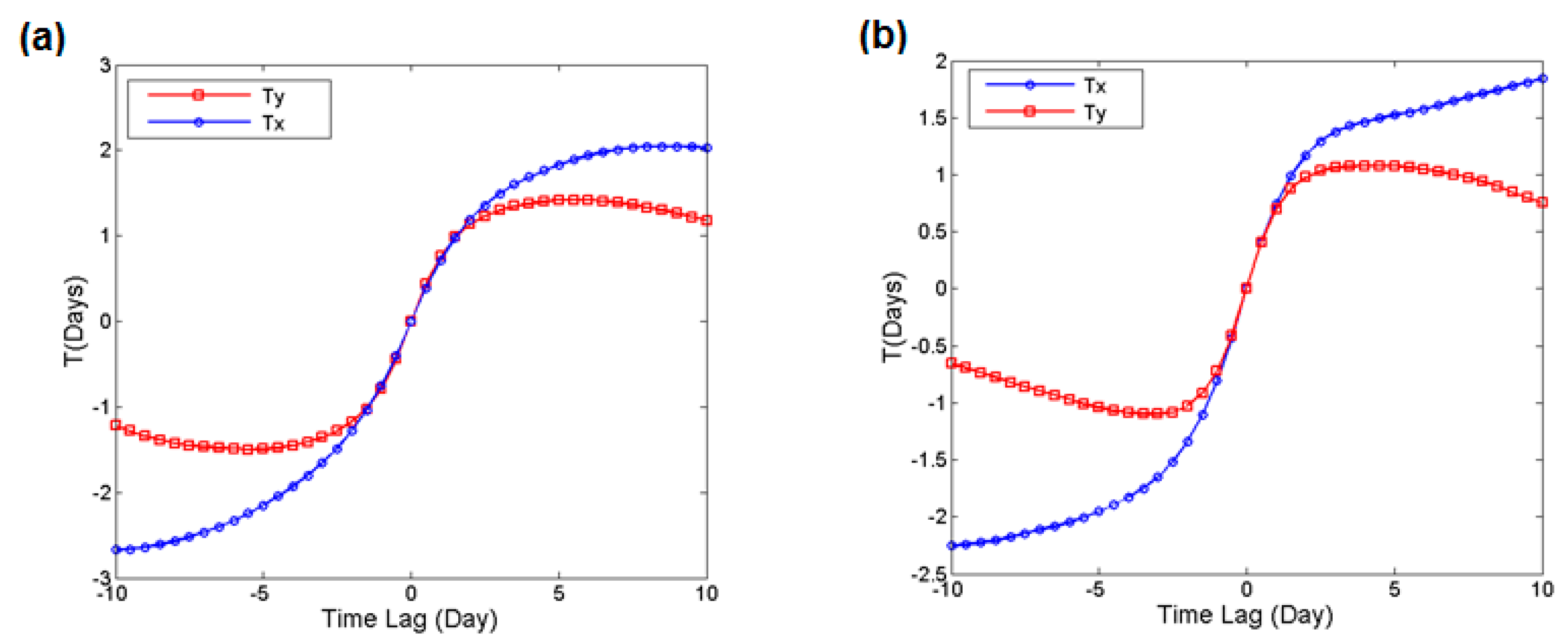
4]. Asymptotic values (independent of time lag) were taken as the maximum values over the range of 0 to 10 days. As the results demonstrate, velocity covariance (Figure 9), diffusivity (Figure 10), and integral time scales (Figure 11) are higher in the along-basin direction.
Lagrangian statistics, calculated using the residual velocities, have a limitation related to the spatial inhomogeneity of fluctuations that are more intense in the boundary areas, as indicated by Poulain (1999).
Figure 9 shows that the variance at zero time lag reaches over 78 (35) ×   10 10   k m 2   s 2 in 2007 and 75 (40) ×   10 10   k m 2   s 2 in 2008 in the along- and across-basin directions, respectively. The results indicate that the velocity covariance has an exponential behavior, where the e-folding time scales in the along- and across-basin directions are approximately 2 and 1.3 days, respectively, during both years. It should be noted that the physical meaning of velocity covariance shows up to which time scales the particle fluctuations play an important role and have a clear and significant effect on transport properties of the sea surface; after the mentioned time scale, the particle velocity will be defined and will be in correspondence with the climatology that is represented by the mean of the flow fields, “U”. Additionally, the results showthat the off-diagonal elements of the covariance matrix are mostly negative.
Furthermore, the variance values obtained by the model (Figure 9) during both years were close to what was observed by Ursella et al. (2006), although these values, especially in the along-basin direction, do not vanish after time lags longer than 10 days. This situation is related to the computation of residual velocity, since it can be affected by large-scale or seasonal residuals; in other words, some low-value frequency errors exist in the residual velocity, which work as a barrier for the convergence of the velocity covariance.
The along-basin diffusivity reaches extreme values of 1.45 ×   10 3   k m 2   s 1 and 1.40 ×   10 3   k m 2   s 1 after approximately 10 days during 2007 and 2008 (Figure 10). In the across-basin direction, the values are smaller (maximum diffusivity less than 0.5 ×   10 3   k m 2   s 1 after four days in 2007 and 0.4 ×   10 3   k m 2   s 1 after three days in 2008); however, for larger time lags, the diffusivity decreases relative to the time lag (Figure 10a,b). Additionally, the effects of low-frequency fluctuations, which were not removed from the residual velocity, were more visible in the diffusivity results, since they did not converge to a constant value.
Figure 11 presents the values of the Lagrangian time scale, which is defined as the time that a drifter remembers its path. The maximum Lagrangian integral time scales are about 2.05 (1.45) days in the along (across)-basin direction in 2007 and 1.85 (1) days for the along (across)-basin direction in 2008. These values are close to the e-folding time scales obtained through the calculation of velocity covariance.
Figure 12 (left upper panel) shows the values of velocity covariance in the along (across)-basin direction for numerical particles during 2007 and 2008 versus drifter data. In the across-basin direction, velocity covariance values obtained from synthetic drifters in both years display the same behaviors, considering that for all time lags they are lower than the drifter data; however, in the along-basin direction, the velocity covariance values for numerical particles deployed in 2007 were slightly higher than the drifter observations during the first time lags. In addition, the results confirm that the vortices generated from velocity fields observed by drifter data are stronger and more energetic than the modeled ones; hence, the dispersion properties of the flow obtained by real drifters show more mixing activities than syntactic particles, which leads to high values of EKE with more turbulence instabilities.
The same comparison was done between modeled and drifter diffusivities. In the along-basin direction, drifter diffusivities were lower than the numerical values until the numerical diffusivities reached their maximum values, and thereafter the drifter diffusivities increased more quickly. It should be noted that the modeled diffusivities in 2008 were closer to real drifter quantities than the 2007 values, considering that diffusivities during 2008 were a slightly lower than in the previous year (Figure 12, right upper panel).
In the across-basin direction, the value of Kyy during 2008 was very similar to real drifter observations, although in 2007 different behavior was displayed versus drifter datasets, especially for larger time lags. Additionally, in the across-basin direction, the results show that the diffusivity values in 2007 were greater than in 2008 (Figure 12). Nonetheless, with good approximation, both years had the same conditions during the first time lags; however, the diffusivity values in the across-basin direction during 2008 were nearly equal to the drifter data.
The comparison of Lagrangian time and length scales obtained by numerical observations during 2007 and 2008 with drifter data shows that there is substantial agreement and similarity between the numerical and experimental results. This finding indicates that the time and distance over which real and synthetic drifters remember their paths are almost the same, although there are some negligible differences related to numerical trajectories during 2007 in the across-basin direction (Figure 13). The importance of these quantities was more evident when the simulation of synthetic trajectories was done by the random flight models based on a decomposition of the velocity fields into mean and turbulent components, as discussed by [1,2].

4. Summary and Conclusions

Lagrangian properties obtained from numerical particles were used to quantify the Adriatic Sea surface circulation during two contrasting years (2007 had a mild winter and cold fall, while2008 had a normal winter and hot summer). Synthetic trajectories were computed from the velocity fields obtained by the Adriatic Sea model developed by Querin et al. (2013) using the MITgcm code. In addition, a comparison between numerical observations (during 2007 and 2008) and real drifter datasets was then performed.
Although the mean flow fields obtained from the synthetic particles during 2007 and 2008 show more similarities with drifter observations, as presented in [2], the major difference is in relation to the anticyclonic pattern in the northern Adriatic close to the Gulf of Trieste, which can be detected visibly by drifter flow fields [23], while the yearly mean circulation maps generated by the model in both years do not show this property of the Adriatic Sea. Furthermore, the influence of Siroccowind regimes is more detectable in the SAP because of the high mixing activities of numerical particles in the mentioned area.

4.1. Residence and Transit Times in the Adriatic Sea

The transit time results demonstrate that numerical particles in 2007 needed more than 180 days to travel from the tip of Istria to the Strait of Otranto, but the mean time for synthetic particles in 2008 was about 200 days, which is more in agreement with the results obtained from numerical drifters (210–260 days) by [2].
Consequently, the residence time values were calculated during the two years. The results indicate that residence times (182~185 days) during both years were higher than what was suggested for numerical particles (150–168 days) by [2]. Moreover, the similarity between the residence time values during both years due to different weather conditions was unexpected; nonetheless, data shows that the Po River discharge exhibited larger values in 2008 than in 2007. On the other hand, the effect of intensive non-uniform wind fields (Bora currents) in the northern end of the Adriatic Sea in 2008 was more visible because of the generation of wind-driven recirculation patterns up to the Po River and off of Istria, which creates an isolated cyclonic gyre. The cyclonic gyre forces the numerical particles to stay there for an extended time, while this was not the case in 2007. Hence, the combined effects of these two parameters (wind fields in the Northern Adriatic and Po River discharge) cause the values of residence time to be similar over the entire basin during the two contrasting years, 2007 and 2008.
Additionally, the MKE maps calculated by velocity fields using OGCM help provide a better explanation for the movement and displacement of numerical particles and their mixing activities, especially due to strong boundary currents along the eastern and western sides of the Adriatic Sea. It should be noted that the vortices generated in the mentioned areas allow the numerical particles to move faster, reducing their residence and transit times in the basin.

4.2. Lagrangian Statistics

The results indicate that the along-basin diffusivities during both years were typically more than twice the size of those in the across-basin direction, considering that the maximum value of the along-basin diffusivity was approximately 1.40 during 2007 and 2008, while these parameter values in the across-basin direction ranged between 0.4   ×   10 3   k m 2   s 1 and 0.5 ×   10 3   k m 2   s 1 for the selected time durations.
Furthermore, it can be determined that the simulated diffusivities were in fairly good agreement with drifter observations. On the other hand, the MKE values during 2008 were slightly higher than those in 2007, although the Adriatic diffusivities were mostly similar during both years. This proves that diffusivities tend to be more affected by the mean EKE. It should be noted that the yearly average values for the EKE were 2.56   ×   10 9 and 2.89   ×   10 9 k m 2   s 2 in 2007 and 2008, respectively, while the MKE values were 3.14   ×   10 9 and 3.79   ×   10 9 k m 2   s 2 during 2007 and 2008, respectively, in the Adriatic Sea.
The velocity covariance was another subject Lagrangian statistical analysis in this study. My results demonstrate that the exponential character of the velocity covariance changed during both years. My findings indicate that the e-folding timescales were in correspondence with the Lagrangian timescale. In addition, the values of Lagrangian time scales obtained from the model during 2007 and 2008 present good agreement with drifter datasets, as calculated by [4].
The results showed that Lagrangian integral time scales obtained from real drifter datasets and synthetic trajectories in the Adriatic Sea (1–3 days) were smaller than the Eulerian scales (e.g., [31]). This contrast reveals that numerical and real drifters generally move faster between mesoscale features than the advection rate of eddies. It should be added that the Lagrangian integral length scales of 5–10 km can be compared to the mesoscale eddies, as well as the internal Rossby radius of deformation.
As a final point related to this study, the effects of eddies on transport and displacement processes of numerical particles were examined during 2007 and 2008. Two types of vortices were detected in the Adriatic Sea. The first group of eddies, which are generated in the cores of circulation cells, are strong enough to force the numerical particles (located or deployed in the mentioned areas) to stay in the basin for longer periods. This situation significantly increases the residence and transit times in the Adriatic Sea. The other types of eddies, as mentioned previously, are produced by strong boundary currents in the eastern and western flanks of the basin. They are affected by energetic inlet flows from the Ionian Sea and Po River discharge, respectively. These vortices accelerate the movement of numerical particles and cause them to exit from the Adriatic Sea in a shorter time.

Author Contributions

The manuscript was written by S.H. Discussions, methodology, validation, review and writing were done by author of manuscript. The author has read and agreed to the published version of the manuscript.

Funding

This research received no external funding.

Acknowledgments

I would like also to thank all of the people at the National Institute of Oceanography and Experimental Physics (OGS), Ecology and Computational Hydrodynamics in Oceanography group (ECHO), especially Stefano Querin, for providing the MITgcm velocity field data.

Conflicts of Interest

The authors declare no conflict of interest.

Data Availability Statements

The data that support the findings of this study are available from the corresponding author upon reasonable request.

References

  1. Falco, P.; Griffa, A.; Poulain, P.M.; Zambianchi, E. Transport properties in the Adriatic Sea as deduced from drifter data. J. Phys. Oceanogr. 2000, 30, 2055–2071. [Google Scholar] [CrossRef]
  2. Poulain, P.M.; Hariri, S. Transit and residence times in the Adriatic Sea surface as derivedfrom drifter data and Lagrangian numerical simulations. Ocean Sci. 2013, 9, 713–720. [Google Scholar] [CrossRef] [Green Version]
  3. Magaldi, M.G.; Özgökmen, T.M.; Griffa, A.; Rixen, M. On the response of a turbulent coastal buoyant current to wind events: The case of the Western Adriatic Current. Ocean Dyn. 2010, 60, 93–122. [Google Scholar] [CrossRef]
  4. Poulain, P.M. Adriatic Sea surface circulation as derived from drifter data between 1990 and 1999. J. Mar. Syst. 2001, 29, 3–32. [Google Scholar] [CrossRef]
  5. Maurizi, A.; Griffa, A.; Poulain, P.M.; Tampieri, F. Lagrangian turbulence in the Adriatic Sea as computed from drifter data: Effects of inhomogeneity and non-stationarity. J. Geophys. Res. 2004, 109, C04010. [Google Scholar] [CrossRef]
  6. Enrile, F.; Besio, G.; Stocchino, A.; Magaldi, M.G.; Mantovani, C.; Cosoli, S.; Gerin, R.; Poulain, P.M. Evaluation of surface Lagrangian transport barriers in the Gulf of Trieste. Cont. Shelf Res. 2018, 167, 125–138. [Google Scholar] [CrossRef]
  7. Carlson, D.; Griffa, A.; Zambianchi, E.; Suaria, G.; Corgnati, L.; Magaldi, M.; Poulain, P.M.; Russo, A.; Bellomo, L.; Mantovani, C.; et al. Observed and modeled surface Lagrangian transport between coastal regions in the Adriatic Sea with implications for marine protected areas. Cont. Shelf Res. 2016, 118, 23–48. [Google Scholar] [CrossRef]
  8. De Dominicis, M.; Leuzzi, G.; Monti, P.; Pinardi, N.; Poulain, P.M. Eddy diffusivity derived from drifter data for dispersion model applications. Ocean Dyn. 2013, 62, 1381–1398. [Google Scholar] [CrossRef] [Green Version]
  9. Bates, M.L.; Griffies, S.M.; England, M.H. A dynamic, embedded Lagrangian model for ocean climate models, Part II: Idealised overflow tests. Ocean Model. 2012, 59–60, 60–76. [Google Scholar] [CrossRef]
  10. Hu, X.; Myers, P.G. A Lagrangian view of Pacific water inflow pathways in the Arctic Ocean during model spin-up. Ocean Model. 2013, 71, 66–80. [Google Scholar] [CrossRef]
  11. Shah, S.H.A.M.; Heemink, A.W.; Gräwe, U.; Deleersnijder, E. Adaptive time stepping algorithm for Lagrangian transport models: Theory and idealised test cases. Ocean Model. 2013, 68, 9–21. [Google Scholar] [CrossRef]
  12. Petersen, M.R.; Jacobsen, D.W.; Ringler, T.D.; Hecht, M.W.; Maltrud, M.E. Evaluation of the arbitrary Lagrangian–Eulerian vertical coordinate method in the MPAS-Ocean model. Ocean Model. 2015, 86, 93–113. [Google Scholar] [CrossRef] [Green Version]
  13. Prants, S.V.; Ponomarev, V.I.; Budyansky, M.V.; Uleysky, M.Y.; Fayman, P.A. Lagrangian analysis of the vertical structure of eddies simulated in the Japan Basin of the Japan/East Sea. Ocean Model. 2015, 86, 128–140. [Google Scholar] [CrossRef]
  14. Berti, S.; Lapeyre, G. Lagrangian reconstructions of temperature and velocity in a model of surface ocean turbulence. Ocean Model. 2014, 76, 59–71. [Google Scholar] [CrossRef]
  15. Coelho, E.F.; Hogan, P.; Jacobs, G.; Thoppil, P.; Huntley, H.S.; Haus, B.K.; Lipphardt, B.L., Jr.; Kirwan, A.D., Jr.; Ryan, E.H.; Olascoaga, J.; et al. Ocean current estimation using a Multi-Model Ensemble Kalman Filter during the Grand Lagrangian Deployment experiment (GLAD), Virtual Special Issue Gulf of Mexico Modelling—Lessons from the spill. Ocean Model. 2015, 87, 86–106. [Google Scholar] [CrossRef]
  16. Rio, M.H.; Pascual, A.; Poulain, P.M.; Menna, M.; Barceló, B.; Tintoré, J. Computation of a new mean dynamic topography for the Mediterranean Sea from model outputs, altimeter measurements and oceanographic in situ data. Ocean Sci. 2014, 10, 731–744. [Google Scholar] [CrossRef] [Green Version]
  17. Artegiani, A.; Bregant, D.; Paschini, E.; Pinardi, N.; Raicich, F.; Russo, A. The Adriatic Sea general circulation: Part I. Air–sea interactions and water mass structure. J. Phys. Oceanogr. 1997, 27, 1492–1514. [Google Scholar] [CrossRef]
  18. Artegiani, A.; Bregant, D.; Paschini, E.; Pinardi, N.; Raicich, F.; Russo, A. The Adriatic Sea general circulation: Part II. Baroclinic Circulation Structure. J. Phys. Oceanogr. 1997, 27, 1515–1532. [Google Scholar] [CrossRef]
  19. Feruglio, G. Risultati di Esperienze con Gallegianti per lo Studio delle Correnti del Mare Adriatico Negli Anni 1910–1914; Appendice: Feruglio, G.—DE MARCHIL. Le Correnti Dell’adriatico Seconodo la Distribuzione Superficial Della Salsedine Della, Paperback—January 1, 1920. Available online: https://www.amazon.co.uk/Risultati-esperienze-galleggianti-Adriatico-1910-1914/dp/B006GE5D38 (accessed on 3 September 2020).
  20. Mazelle, E. Flachenposten in der Adria zurBestimungen der OberflachenStromungen. Denkschr. Akad. Wiss. Naturwiss. Klasse 1914, 91, 1–46. [Google Scholar]
  21. Orlic, M.; Gacic, M.; La Violette, P.E. The currents and circulation of the Adriatic Sea. Oceanol. Acta 1992, 15, 109–124. [Google Scholar]
  22. Poulain, P.M. Drifter observations of surface circulation in the Adriatic Sea between December 1994 and March 1996. J. Mar. Syst. 1999, 20, 231–253. [Google Scholar] [CrossRef]
  23. Ursella, L.; Poulain, P.M.; Signell, R.P. Surface drifter derived circulation in the northern and middle Adriatic Sea: Response to wind regime and season. J. Geophys. Res. 2006, 111, C03S04. [Google Scholar] [CrossRef]
  24. Marshall, J.; Adcroft, A.; Hill, C.; Perelman, L.; Heisey, C. A finite-volume, incompressible Navier Stokes model for studies of the ocean on parallel computers. J. Geophys. Res. 1997, 102, 5753–5766. [Google Scholar] [CrossRef] [Green Version]
  25. Tonani, M.; Pinardi, N.; Dobricic, S.; Pujol, I.; Fratianni, C. A high resolution free surface model on the Mediterranean Sea. Ocean Sci. 2008, 4, 1–14. [Google Scholar] [CrossRef] [Green Version]
  26. Querin, S.; Crise, A.; Deponte, D.; Solidoro, C. Numerical study of the role of wind forcing and freshwater buoyancy input on the circulation in a shallow embayment (Gulf of Trieste, Northern Adriatic Sea). J. Geophys. Res. 2006, 111, C03S16. [Google Scholar] [CrossRef]
  27. Querin, S.; Cossarini, G.; Solidoro, C. Simulating the formation and fate of dense water in a mid-latitude marginal sea during normal and warm winter conditions. J. Geophys. Res. Oceans 2013, 118, 885–900. [Google Scholar] [CrossRef]
  28. Cossarini, G.; Querin, S.; Solidoro, C. The continental shelf carbon pump in the northern Adriatic Sea (Mediterranean Sea): Influence of wintertime variability. Ecol. Model. 2015, 314, 118–134. [Google Scholar] [CrossRef] [Green Version]
  29. Davis, R.E. Observing the general circulation with floats. Deep-Sea Res. 1991, 38 (Suppl. 1), S531–S571. [Google Scholar] [CrossRef]
  30. Cushman-Roisin, B.; Gacic, M.; Poulain, P.-M.; Artegiani, A. Physical Oceanography of the Adriatic Sea Past, Present and Future; Kluwer Academic: Dordrecht, The Netherlands, 2001. [Google Scholar]
  31. Kovacevic, V.; Gacic, M.; Poulain, P.-M. Eulerian current measurements in the Strait of Otranto and in the Southern Adriatic. J. Mar. Syst. 1999, 20, 255–278. [Google Scholar] [CrossRef]
  32. Danovaro, R.; Boero, F. Italian seas. In World Seas. An Environmental Evaluation, 2nd ed.; Sheppard, C., Ed.; Academic Press: London, UK, 2019; pp. 283–306. [Google Scholar]
Figure 1. Mean flow fields and circulation cells in the Adriatic Sea obtained by numerical particles in this study during 2007 (a), 2008 (b), and the example of study area (c), for more details about the maps of study area see: [32]).
Jmse 08 00681 g001aJmse 08 00681 g001b
Figure 2. Values for the kinetic energy of the mean flow (MKE) ( k m 2 s 2 ) in 2007 (a) and 2008 (b).
Jmse 08 00681 g002
Figure 3. Wind speed distribution (m/s) in the Adriatic Sea during (a) March 2007, (b) March 2008, (c) December 2007, and (d) December 2008.Colorbar shows selected range for the wind speed (m/s).
Jmse 08 00681 g003
Figure 4. Mean time to exit the Strait of Otranto (days) for numerical particles during 2007 (a) and 2008 (b).
Jmse 08 00681 g004
Figure 5. Po River discharge during 2007 and 2008 ( m 3 s ).
Jmse 08 00681 g005
Figure 6. Monthly average of the Po River discharge during all examined years, 2006 to 2011 ( m 3 s ).
Jmse 08 00681 g006
Figure 7. Wind speed distributions (m/s) in the northern Adriatic Sea (the northernmost area: the Gulf of Trieste) during (a) March 2007, (b) March 2008, (c) December 2007, and (d) December 2008. Colors in boxes show the selected range for the wind speed (m/s).
Jmse 08 00681 g007aJmse 08 00681 g007b
Figure 8. Residence time T* (days) values versus time for numerical particles in 2007 and 2008.
Jmse 08 00681 g008
Figure 9. Lagrangian statistic (velocity covariance) calculated for the entire Adriatic basin after removal of the mean Eulerian circulation. Statistics are shown versus time lags ranging between −10 and 10 days for numerical particles in 2007 (a) and 2008 (b). (Pxx and Pyy show along and across basin velocity covariance values respectively).
Jmse 08 00681 g009
Figure 10. Lagrangian statistics (diffusivity) calculated for the entire Adriatic basin after removal of the mean Eulerian circulation. Statistics are shown versus time lags ranging between −10 and 10 days for numerical particles in 2007 (a) and 2008 (b). (Kxx and kyy show along and across basin diffusivity values respectively).
Jmse 08 00681 g010
Figure 11. Lagrangian statistics (integral time scale) are shown versus time lags ranging between −10 and 10 days for numerical particles in 2007 (a) and 2008 (b).
Jmse 08 00681 g011
Figure 12. Comparison between the Lagrangian statistics in 2007 and 2008 and real drifter data (a) velocity covariance (b,c) diffusivity, Lagrangian integral length scale and Lagrangian integral time scale.
Jmse 08 00681 g012aJmse 08 00681 g012b
Figure 13. Comparison between the Lagrangian statistics in 2007 and 2008 and real drifter data (a) velocity covariance (b) diffusivity, Lagrangian integral length scale, and Lagrangian integral time scale).
Jmse 08 00681 g013
Table 1. Comparison between the Lagrangian parameters [2,4,23].
Residence Time (days)Transit Time (Northern Adriatic-Otranto)Transit Time (Otranto-Otranto)
Real drifters7010083
Synthetic drifters in 2007182166155
Synthetic drifters in 2008185168143
Numerical drifter ([2], turbulence: [4])168260185
Numerical drifter ([2], turbulence: [23])150216170
Table 2. Lagrangian statistics for the whole Adriatic basin during 2007 and 2008 using synthetic trajectories compared with real drifter datasets.
Variance   ( c m 2   s 2 ) Diffusivity   ( c m 2   s 1 ) Lagrangian Integral Time (Days)Lagrangian Integral Length Scale (km)
DirectionAlong AcrossAlong AcrossAlong AcrossAlong Across
Real drifters106.31.92.118.4
70.30.71.17.9
Synthetic drifters in 2007851.452.0513
350.51.454.15
Synthetic drifters in 2008701.41.8514.8
400.416

