Power Prediction of Wind Farms via a Simplified Actuator Disk Model

Abstract

This paper aims to demonstrate a simplified nonlinear wake model that fills the technical gap between the low-cost and less-accurate linear formulation and the high-cost and high-accuracy large eddy simulation, to offer a suitable balance between the prediction accuracy and the computational cost, and also to establish a robust approach for long-term wind farm power prediction. A simplified actuator disk model based on the momentum theory is proposed to predict the wake interaction among wind turbines along with their power output. The three-dimensional flow field of a wind farm is described by the steady continuity and momentum equation coupled with a k-$\epsilon$ turbulence model, where the body force representing the aerodynamic impact of the rotor blade on the airflow is uniformly distributed in the Cartesian cells within the actuator disk. The characteristic wind conditions identified from the data of the supervisory control and data acquisition (SCADA) system were employed to build the power matrix of these typical wind conditions for reducing the computation demands to estimate the yearly power production. The proposed model was favorably validated with the offshore measurement of Horns Rev wind farm, and three Taiwanese onshore wind farms were forecasted for their yearly capacity factors with an average error less than 5%, where the required computational cost is estimated about two orders of magnitude smaller than that of the large eddy simulation. However, the proposed model fails to pronouncedly reproduce the individual power difference among wind turbines in the investigated wind farm due to its time-averaging nature.

1. Introduction

The growing demand for wind energy has greatly enhanced the fast development of large-scale wind farms, especially in the offshore sectors. The weather research and forecasting (WRF) model [1,2] germinated in the late 1990s is a widely adopted tool to evaluate the atmospheric condition for a given area, and to assess its corresponding wind energy potential [3,4]. After the site for a planned wind farm has been determined via a proper wind resource assessment and evaluation, the decision around wind turbine location in the wind farm becomes the next key task before the related construction and installation work can begin. However, the wind turbine array installed generally suffers from various degrees of power loss due to the wake interaction among neighboring wind turbines. In order to efficiently harvest the wind energy captured by wind turbines installed in a wind farm, the wake interaction between the upstream and downstream wind turbines has to be accurately forecasted for maximizing the power production of a wind farm through an appropriate wind turbine siting. Three major numerical models have been proposed to identify the impact of the upstream wake on the downstream wind turbines, alongside the resulting power deficiency. The analytical model based on the conservation of momentum that arose in the 1980s is the most simple and efficient model to predict the downstream wind speed evolution of a single wind turbine [5,6], and this linear approach is further applied to the estimation of the complex shadow effects behind multiple upstream wind turbines [7]. One major drawback of this approach is to assume a linear wake decay along the flow direction that is rarely observed in the field cases characterized by non-trivial turbulence. Additionally, this model is also criticized for not being self-consistent because it uses an empirical constant to describe the downstream wake expansion behavior as well as the prediction accuracy being heavily dependent on a reasonable estimation of the wake recovery behavior. When the wind turbine is not aligned with the wind direction, the substantial flow angle leads to a downstream wake with high degree of nonlinearity, where the linear model obviously loses its validity. Despite these drawbacks, this approach has been broadly employed in the early planning stage of wind farm development due to its efficiency. A computational fluid dynamics (CFD) model with the detailed wind turbine geometry resolved in the flow domain, i.e., a full CFD model, also serves as a popular approach to investigate the nonlinear flow around wind turbines. Owing to being capable of delivering the temporal flow details in space, this approach is widely adopted to study the aerodynamic and aeroacoustic characteristics of single wind turbines [8,9,10]. The full CFD model is able to model the wake flow in a self-consistent way because the flow nonlinearity, together with the turbulence transport, is well considered in the related governing equations. However, it apparently becomes impractical in the flow prediction of massive wind farms with large number of wind turbines due to the complexity in grid generation and the accompanied computational cost [11]. Nowadays, the most prevalent nonlinear approach to simulate wind farm flow is the CFD approach incorporated with a body force model where the rotor geometry is fully neglected in a Cartesian grid system and replaced by a force distribution in space to account for the aerodynamic force of the rotor blades exerted on the incoming airflow [12,13]. In this approach, the blade element momentum (BEM) theory [14] is adopted to estimate the body force distribution in space by using the flow condition at the blade section location to obtain the corresponding lift and drag coefficient from a pre-defined aerodynamics table. Large eddy simulation (LES) [15,16] is a state-of-art model in this category, where a precursor calculation is first conducted for the flow domain to create the required unsteady turbulent inflow condition within a fixed period followed by a transient wind farm modeling with the designated body force distribution from the BEM model to represent the aerodynamic impact of the wind turbines on the airflow. In addition to a self-consistent nature in turbulence, the ability to offer a fine temporal resolution of turbulence in space, especially the contribution of large eddies, serves as the main cause of its great popularity. By contrast, the length modeling time of its unsteady process together with the high computational cost to resolve the eddies embedded in the flow field is regarded as the main technical barrier to prevent it from serving as an affordable design tool. Due to this numerical feature, LES is prone more employed in the diagnostic or validation cases rather than in the early or design stage of wind farm development. The motivation of this paper is to bridge the low-cost and less-accurate linear model and the high-cost and high-accuracy nonlinear model via a proposed simplified nonlinear model that provides a reasonable balance between the prediction accuracy and the computational cost. When an average power output of wind farms or wind turbines is of main interest, such as in the design stage or in a long-term prediction for estimating the capacity factor, a nonlinear steady actuator-disk model offers a very promising solution to acquire sufficient accuracy with economical computation expense. In this study, a simplified actuator disk model based on the momentum theory is proposed to model the flow around and across wind turbines while an accompanied approach to efficiently forecast the yearly capacity factor of a wind farm is further demonstrated. The proposed approach is first validated by the power measurements of Horns Rev offshore wind farm under different wind conditions. Three Taiwanese onshore wind farms are then employed to verify the accuracy of the proposed approach in the forecast of yearly capacity factor.

2. Mathematical Model

2.1. Governing Equations

It is assumed that the flow field in a wind farm is incompressible and steady, where gravity and temperature effects are fully neglected. The continuity and Reynolds-Averaged Navier-Stokes (RANS) equations are given as follows:

$$\frac{\partial u_i}{\partial x_i}=0,$$

(1)

$$u_j\frac{\partial u_i}{\partial x_j}=-\frac{1}{\rho }\frac{\partial p}{\partial x_i}+\upsilon \frac{{\partial }^2{u}_i}{\partial x_i\partial x_j}-\frac{\partial \overline{u_i^{’}{u}_j^{’}}}{\partial x_j}+f_i,$$

(2)

where $\rho$ denotes the density, $p$ the pressure, $\upsilon \left(={\upsilon }_m+{\upsilon }_t\right)$ the effective kinematic viscosity, ${\upsilon }_m$ the kinematic viscosity, ${\upsilon }_t$ the turbulent kinematic viscosity, $\overline{u_i^{’}{u}_j^{’}}$ the Reynolds stress, $f_i$ the body force representing the aerodynamic characteristic of rotor. A k-$\epsilon$ turbulence model was adopted in this study. The transport equation of turbulent kinetic energy (k) and its dissipation rate ($\epsilon$) are shown as follows [17]:

$$\frac{\partial }{\partial x_j}\left(k{u}_j\right)=\frac{\partial }{\partial x_j}\left(\left(\upsilon +\frac{{\upsilon }_t}{{\sigma }_k}\right)\frac{\partial k}{\partial x_j}\right)+P_k-\epsilon ,$$

(3)

$$\frac{\partial }{\partial x_j}\left(\epsilon u_j\right)=\frac{\partial }{\partial x_j}\left(\left(\upsilon +\frac{{\upsilon }_t}{{\sigma }_{\epsilon }}\right)\frac{\partial \epsilon }{\partial x_j}\right)+c_{\epsilon 1}{P}_k\frac{\epsilon }{k}-c_{\epsilon 2}\frac{{\epsilon }^2}{k},$$

(4)

$${\upsilon }_t=c_{\mu }\frac{k^2}{\epsilon },$$

(5)

$$P_k=-\overline{u_i^{’}{u}_j^{’}}\frac{\partial u_j}{\partial x_j}+P_b,$$

(6)

where $P_k$ represents the total production of turbulent kinetic energy and $P_b$ the production of turbulent kinetic energy due to rotor motion. The equation constants of the turbulence model $\left(c_{\mu },{\sigma }_k, {\sigma }_{\epsilon }, c_{\epsilon 1}, c_{\epsilon 2}\right)$ are given in

Table 1. The equation constants of turbulence model.

${\mathit{c}}_{\mathit{\mu }}$	${\mathit{\sigma }}_{\mathit{k}}$	${\mathit{\sigma }}_{\mathit{\epsilon }}$	${\mathit{c}}_{\mathit{\epsilon }1}$	${\mathit{c}}_{\mathit{\epsilon }2}$
0.09	1.00	1.30	1.44	1.92

. The wall function approach [17] was additionally adopted in this study to properly describe the region bridging the viscos layer and the turbulent region.

2.2. Actuator Disk Model

In the proposed simplified actuator disk model, the wind turbine geometry is fully neglected in the computational domain [18]. Instead, the blade force acting on the incoming airflow is modeled via an extra body force term, i.e., $f_i$, in the momentum equations in the swept region of rotor where the body force distribution following the aerodynamic characteristics of rotor under specific wind conditions is prescribed [19,20,21]. Similar to the body force term, a turbulence source term, i.e., $P_b$, representing the turbulence generated by the rotor motion is additionally applied to the Cartesian cells residing within the swept region in the solution of turbulent kinetic energy k. In the proposed actuator disk model, the geometric parameters describing the wind turbine are the rotor diameter ($D$) and the hub height ($H$). The operation parameters describing the wind turbine are the rotor angular velocity ($\omega$), the output power ($P$), and the average axial velocity at rotor ($U_{AVE}$).

2.3. Body Force Distribution

The body force assigned to the cell in the swept region can mainly be decomposed into an axial component and a tangential component. The radial component is too small to be included in the body force term when compared to other two components. Due to the blades steadily sweeping over the space of the actuator disk at a specific speed, the body force distribution is therefore equally distributed in the azimuthal direction to represent a time-averaging effect of the rotor force acting on the incoming airflow. The body force distribution along the radial direction theoretically has to comply with the aerodynamic performance of airfoils varying along the radial direction. Prior knowledge of the blade geometry is therefore necessary to determine the correct radial variation of body force. However, this information is frequently inaccessible because of a planned power output instead of a wind turbine solution being generally available in the early design stage or the geometric details of the installed wind turbine being unattainable in many cases. Because the wake variation in the radial direction benefits from the turbulent mixing quickly attenuating along the downstream distance, the wake with a growing uniformity is expected to develop at the rotor disk of downstream locations. This wake behavior can be easily modelled by a uniform body force distribution in the radial distribution, provided that the far wakes, such as those taking place in a wind farm having multiple wind turbines arranged in rows or columns, are of main interest. Thus, a constant body force density results over the rotor disk.

Based on the momentum theory, the total axial force that the rotor disk exerts on the incoming airflow ($F_a$) is estimated from the power of wind turbine and the average axial velocity component of the airflow across the rotor:

$$U_{AVE}=\frac{1}{A}{\displaystyle \int }UdA,$$

(7)

$$F_a=\frac{P}{U_{AVE}},$$

(8)

where $U$ is the axial flow velocity and $A$ the swept area of the rotor disk. The accompanied axial force density ($f_a$) is defined by the following equation:

$$f_a=\frac{4P}{\pi R{D}^2{U}_{AVE}},$$

(9)

where $R$ denotes the rotor radius. The rotor torque ($Q$) contributed by the incoming airflow to drive the rotor operating at a rotor speed of $\omega$ is given as follows:

$$Q=\frac{P}{2\pi \omega }.$$

(10)

The accompanied tangential force density ($f_t$) is then obtained from the identity of the rotor torque with the surface integral contributed by the tangential body force:

$$f_t=\frac{6P}{{\pi }^2{D}^3\omega }.$$

(11)

The power curve of a wind turbine, Figure 1a, only depicts the correlation between the undisturbed incoming wind speed ($V$) and its power output where no related information of the axial velocity component across the rotor is disclosed. It is necessary to define the average axial velocity of airflow across the rotor as a function of power and rotor speed for the operation range before the evaluation of body force density via Equations (9) and (11) is possible in any wake prediction of the wind farm. Therefore, the correlation among $U_{AVE}$, $\omega$ and $P$ has to be established in order to enable the body force calculation. A single wind turbine is initially adopted to discover the required correlation among $U_{AVE}$, $\omega$ and $P$. With a given inflow velocity, the corresponding rotor speed and power are obtained from the power curve. These two values are directly enforced in the flow simulation and the average axial velocity component is then evaluated by Equation (7) after a converged solution of the flow field is attained. A correlation among $U_{AVE}$, $\omega$ and $P$ for the full operation range is subsequently established with the help of a comprehensive flow simulation under various inflow conditions defining a power curve. Figure 1b illustrates the correlation among $U_{AVE}$, $\omega$ and $P$ for the wind turbine V80 with the aforementioned approach. In this study, the power curve governing the wind turbine power characteristics is explicitly replaced by the dependence of $P$ and $\omega$ on $U_{AVE}$ that is adopted to determine the power behavior of wind turbines for feasible wind conditions.

The body force is first distributed over the rotor disk based on a prescribe arrangement of disk elements with the abovementioned force density and the force on disk elements is further distributed to the neighboring Cartesian cells. In the definition of disk elements, the rotor disk is divided into I radial segments and J circumferential segments. The disk element is represented by its geometric center, appearing as the red point in Figure 2a. For simplicity, the disk element is homogenously distributed along the radial and circumferential direction over the rotor disk. The body force acting on a disk element is hence expressed as

$$f=\left(f_{a}S\right)e_a+\left(f_{t}S\right)e_t,$$

(12)

where $S$ is the area of a disk element, $e_a$ the unit normal vector in the axial direction and $e_t$ the unit normal vector in the tangential direction. Due to numerical reasons, the body force of a disk element is only distributed within a finite region. Only the Cartesian cells with a distance ($d$) to the target disk element smaller than a given value ($ϵ$) is considered in the body force distribution. Figure 2b depicts the distribution of body force from a disk element to its neighboring Cartesian cells defined by the black crosses. The weighting of body force distribution among neighboring Cartesian cells is governed by a Gaussian distribution, ${\eta }_{ϵ}\left(d\right)$:

$${\eta }_{ϵ}\left(d\right)=\frac{1}{{ϵ}^2{\pi }^{2/3}}\exp \left[-{\left(\frac{d}{ϵ}\right)}^2\right].$$

(13)

Therefore, the body force applied to a Cartesian cell $f_{ϵ}$ is expressed as follows:

$$f_{ϵ}={{\displaystyle \sum }}_k{f}_k{\eta }_{ϵ},$$

(14)

where $f_k$ denotes the body force of a disk element that is distant less than $ϵ$ from the Cartesian cell.

3. Numerical Method

3.1. Solution Process

In the method proposed in this study, an in-house code is implemented for the wake flow prediction of wind farms based on the proposed mathematical model where a linear domain decomposition scheme is employed to parallelize the flow computation on a Cartesian gird via the MPI library [22]. A second-order finite volume method based on a deferred correction approach is adopted to discretize the governing equations and a semi-implicit method for pressure-linked equations (SIMPLE) algorithm is employed to decouple velocity and pressure. During the outer iteration of a flow computation, the velocity fields are predicted by solving the momentum equations. After the correction of mass flux at the outlet boundary, the velocity and pressure fields are updated through the pressure correction obtained from solving the continuity equation. The turbulence model is subsequently solved for the turbulence property of the flow field. In the inner iteration of a flow computation, the linearized equations are solved via a strongly implicit procedure (SIP) solver [23] to determine the field variables. Figure 3 shows the solution procedure of the proposed numerical method, as well as the corresponding in-house code, WIFA3D. The flow calculation is considered to be converged when the normalized residual of governing equations is smaller than ${10}^{-3}$ during an iterative solution process.

3.2. Computational Domain

The typical computational domain adopted in this study has the shape of a rectangular box that principally targets offshore wind farms or inland wind farms on flat terrain, such as the onshore wind farms near coastlines demonstrated in the later sections. The computational domain is demonstrated in Figure 4, where the blue-line region explicitly defines the boundary of the interested wind farm. The origin is defined at the center of the wind farm. The symbols a to h label the corners of the computational domain that is featured with a width of $L_1$ alongside a height of $L_2$. The distance between the inflow boundary (abcd) and the studied wind farm is $L_3$, while the distance between the outflow boundary (efgh) and the investigated wind farm is $L_4$. The values of $L_1, L_2, L_3$, and $L_4$ is properly determined according to the size of a wind farm.

3.3. Boundary Conditions

For the convenience of specifying boundary conditions, the inflow direction is always parallel to the $x$-direction of the coordinate system. The inflow condition is adopted on the boundaries abcd and aefb. The inflow wind speed varying with height is given in the following equation:

$$U_a=U_{\mathrm{in}}{\left(\frac{z}{H}\right)}^{\delta }$$

(15)

where $U_a$ denotes the inflow velocity, $U_{\mathrm{in}}$ the wind velocity at the hub height, $z$ the height measured from the ground,$H$ the hub height, and $\delta$ the index of ground roughness that is set 0.1 for smooth terrains appearing in the offshore or near shore applications [24]. A zero gradient condition is applied to the field variable at the outflow boundary efgh. A symmetry condition is employed on the boundaries aefd and bfgc. A no-slip condition is assigned to the boundary cdhg. The boundary conditions used in this study are summarized in

Table 2. The equation constants of turbulence model.

Boundary	Type	$\mathit{U}$	$\mathit{V}$	$\mathit{W}$
abcd, aefb	Inlet	(Equation (15))	0	0
aehd, bfgc	Slip wall	$\frac{\partial U}{\partial n}=0$	0	$\frac{\partial W}{\partial n}=0$
cdhg	No-slip wall	0	0	0
efgh	Outlet	$\frac{\partial U}{\partial n}=0$	$\frac{\partial V}{\partial n}=0$	$\frac{\partial W}{\partial n}=0$

where $U$, $V$, and $W$ are the velocity components in the $x$, $y,$ and $z$ directions, respectively, and $n$ the normal direction of the boundary.

3.4. Grid Dependence

A Cartesian grid to discretize the computational domain with a grid number of about 8.2 million is schematically shown in Figure 5, where $N_x$, $N_y$, and $N_z$ denotes the grid segments in the x, y, and z direction, respectively. The increase in the grid number apparently helps to deliver more accurate results, but with a high computation cost. Therefore, a grid dependency study was adopted to find the balance between grid number and prediction accuracy. In this study, five grid levels systematically refined from 0.2 million to 32 million cells were chosen to investigate the dependence of $U_{AVE}$ on the grid number. Richardson’s extrapolation was employed to estimate the grid-independent value (${\varphi }_{\infty }$) of a physical quantity ($\varphi$) in a second-order scheme:

$${\varphi }_{\infty }={\varphi }_n+\frac{{\varphi }_n-{\varphi }_{n-1}}{{\left(\sqrt[3]{\frac{N_n}{N_{n-1}}}\right)}^2-1},$$

(16)

where ${\varphi }_n$ and ${\varphi }_{n-1}$ are the physical quantity of the $n$th and ($n-1$)th grid levels, respectively, and $N_n$ and $N_{n-1}$ are the grid number of the $n$th and ($n-1$)th grid levels, respectively. The average wind speed at the rotor disk of the wind turbine V80 under a wind speed of 5 m/s was surveyed for its grid dependency. The rated wind speed Figure 6a shows that the average wind speed at the rotor disk gradually converges to a grid-independent solution of 4.922 m/s as the number of grid ($N_x\times N_y\times N_z$) steadily grows. The dimensionless grid size ($dx$) along with the discretization error ($E_{\varphi }$) is given as follows:

$$x=\sqrt[3]{\frac{1}{N}},$$

(17)

$$E_{\varphi }=\left|\frac{{\varphi }_{\infty }-\varphi }{{\varphi }_{\infty }}\right|,$$

(18)

where $N$ is the grid number. Figure 6b shows the discretization error of $U_{AVE}$. on various grids. The third grid level with a grid number of 8.2 million gives a discretization error of $U_{AVE}$ in 0.46%. This clearly suggests that the proposed approach has good numerical consistency and sufficient numerical stability. The role of grid spacing in three directions is governed by their individual purpose. The grid distribution of the vertical coordinate is focused on a good representation of the near-wall viscous layer where substantial velocity gradient along the vertical direction is expected, as well as a smoother velocity profile at higher altitude. The longitudinal and horizonal grid spacing is used to capture the wake variation across the rotor, while the former additionally keeps track of the downstream wake evolution. Based on this consideration, the grid is vertically clustered near the solid wall to adapt to the wall function employed in this study accompanied by an appropriate expansion rate to reach a nearly uniform size in the actuator disk for accurately resolving the airflow across the rotor. A similar grid spacing is generally used within the actuator disk for both horizontal and vertical direction and this grid size is also adopted in the longitudinal direction. This grid practice aimed to minimize the additional numerical diffusion caused by the excessive aspect ratio of grid size.

4. Numerical Results

4.1. Validation of Horns Rev Wind Farm

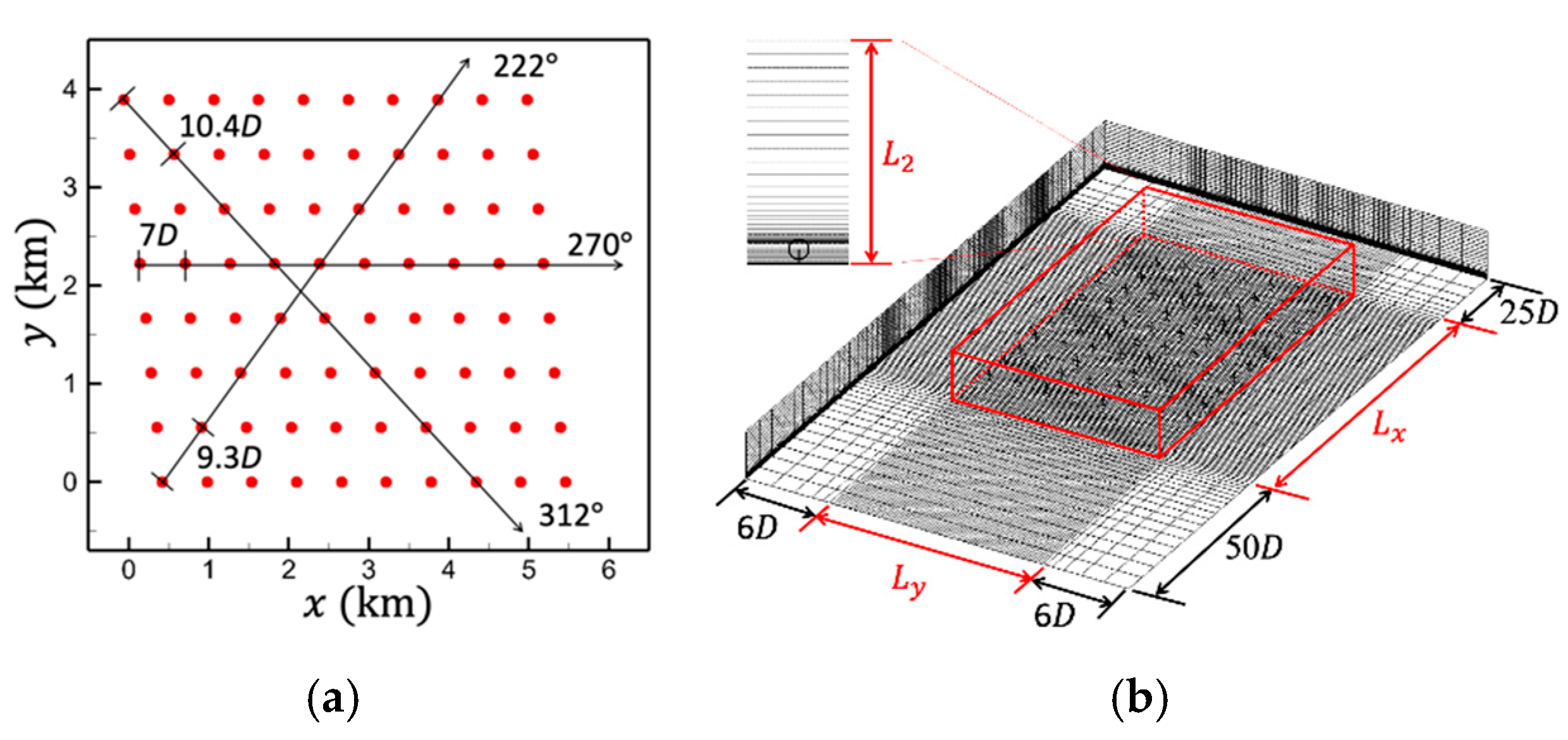
This study first predicts the power output of Horns Rev wind farm for a wind speed of 8 m/s with three distinct wind directions. The wind turbine layout of Horns Rev wind farm is shown in Figure 7a, where the red solid dots represent the locations of the installed Vestas V80 wind turbines. Three specific wind directions ($\alpha =220°$, $270°$, and $312°$) corresponding to a tower spacing (d) of 9.3$D$, 7$D$, and 10.4$D$ are selected as the validation cases. 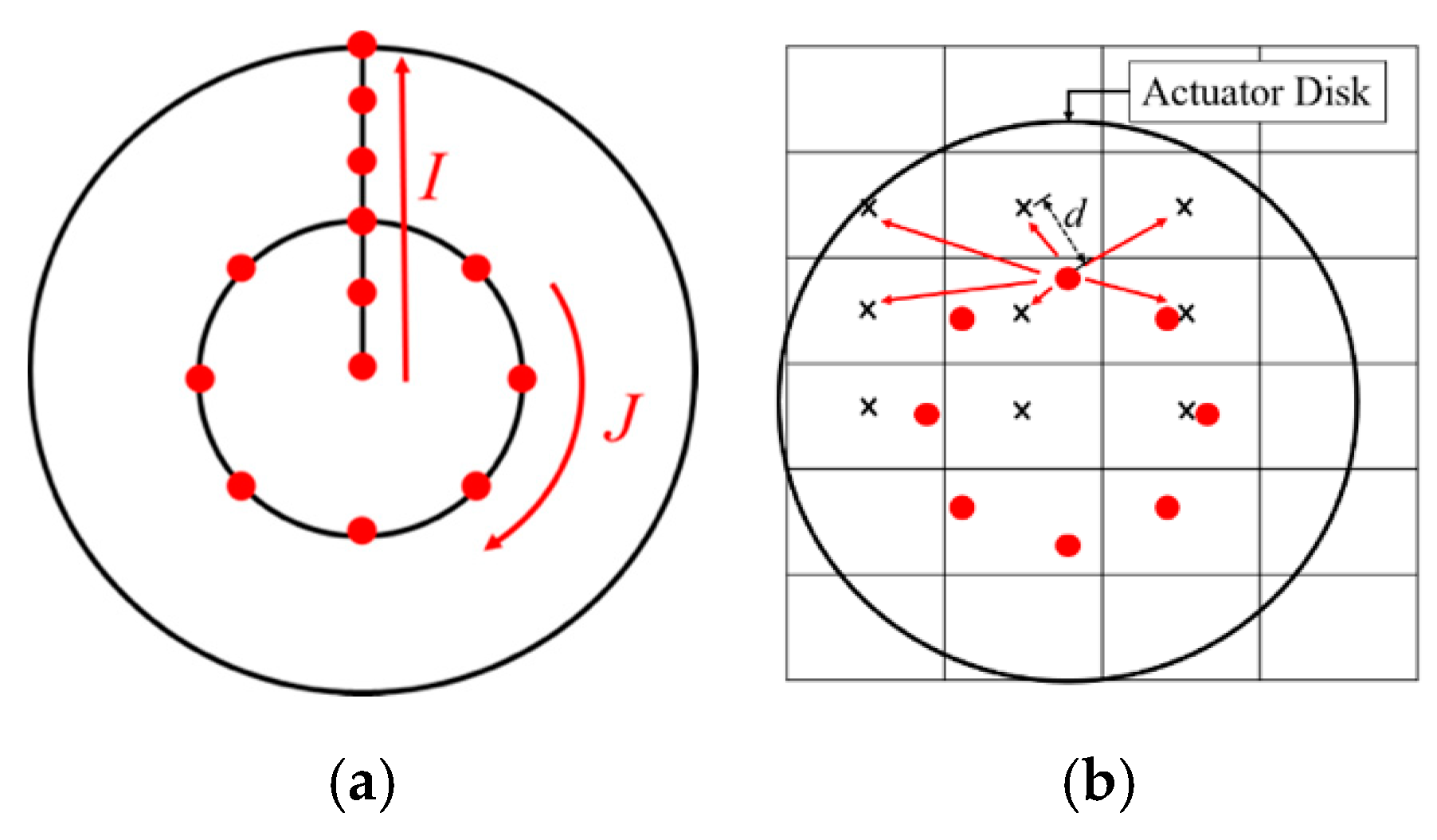Figure 7b illustrates the typical grid arrangement for the Horns Rev wind farm, where $L_x$ is the longitudinal size of the wind farm, $L_y$ the lateral size of the wind farm, $L_1=L_y+12D, L_2=12.5D, L_3=25D$ and $L_4=50D$. 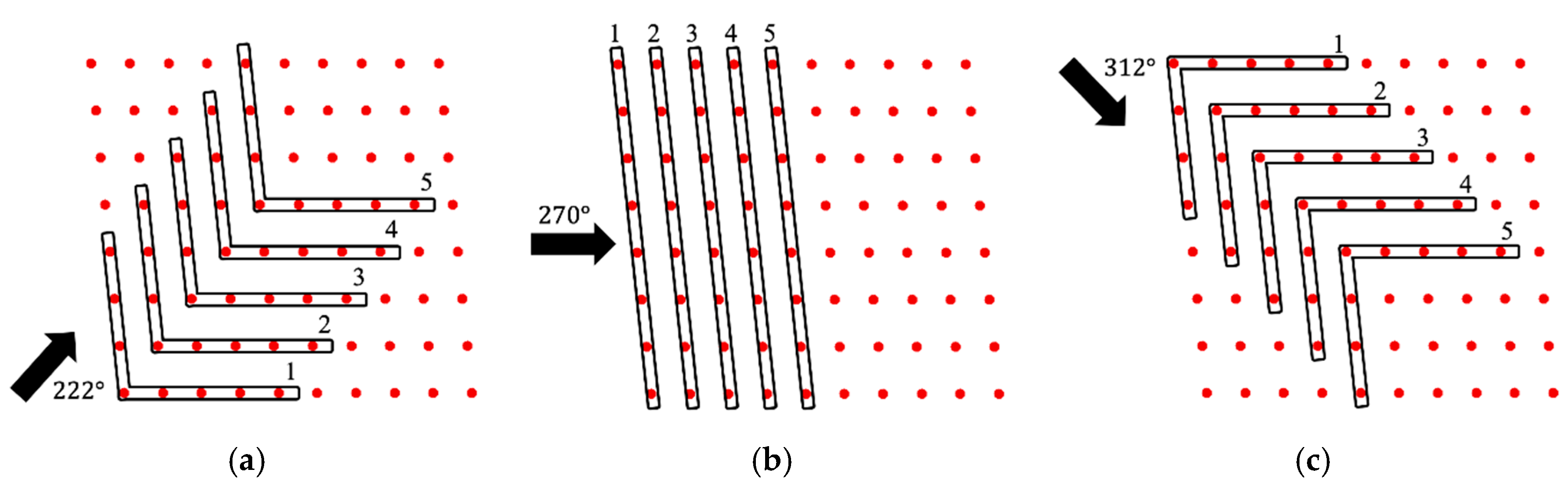The numerical mesh was particularly clustered in the region where the rotor of a wind turbine is located. Two different domain sizes, i.e., a full model and a reduced one, are additionally compared to identify their computational advantages and drawbacks in the power prediction of wind farms. 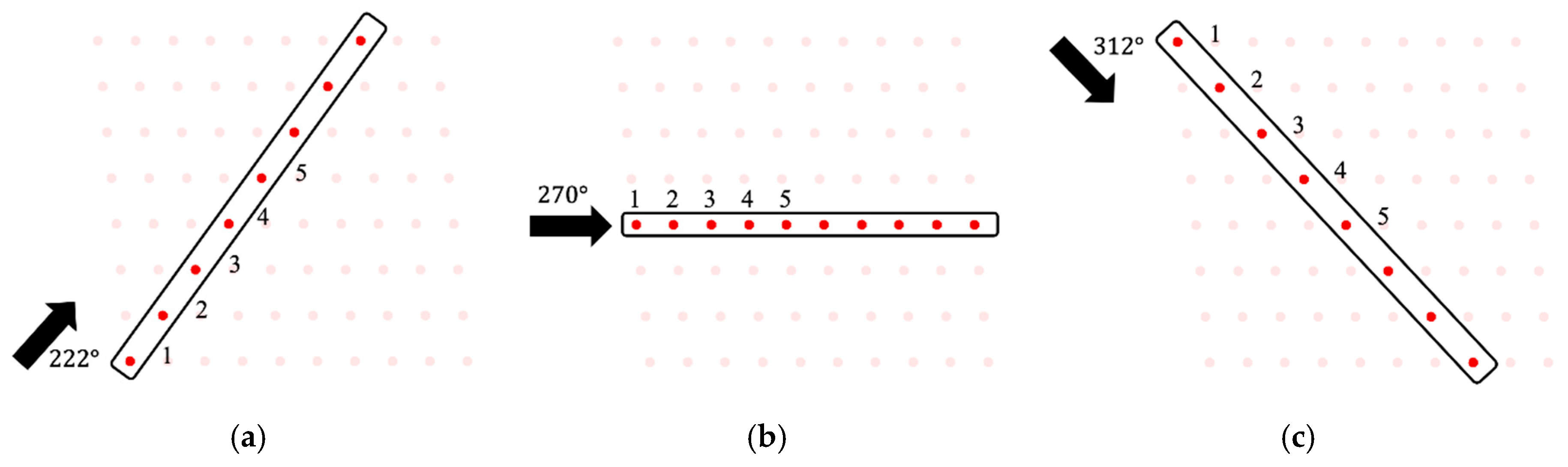In the full model, a complete wind farm is simulated, Figure 8, whereas the reduced model only considers a cascading wind turbine arrangement due to the tower location symmetry of the investigated wind turbine array, Figure 9.

Table 3. Grid parameters adopted for the full model of the Horns Rev wind farm.

$\mathit{\alpha }$	${\mathit{L}}_{\mathit{x}}/\mathit{D}$	${\mathit{L}}_{\mathit{y}}/\mathit{D}$	$\mathit{d}\mathit{x}\left(\mathbf{m}\right)$	$\mathit{d}\mathit{y}\left(\mathbf{m}\right)$	$\mathit{d}\mathit{z}\left(\mathbf{m}\right)$	$\mathit{d}{\mathit{z}}_0\left(\mathbf{cm}\right)$	${\mathit{N}}_{\mathit{r},\mathit{y}}$	${\mathit{N}}_{\mathit{r},\mathit{z}}$	${\mathit{N}}_{\mathit{x}}\times {\mathit{N}}_{\mathit{y}}\times {\mathit{N}}_{\mathit{z}}$
222°	85	90	8	8	8	10	10	10	850$\times$900$\times$55
270°	81	55							810$\times$550$\times$55
312°	95	80							950$\times$800$\times$55

and

Table 4. Grid parameters adopted for the reduced model of Horns Rev wind farm.

$\mathit{\alpha }$	${\mathit{L}}_{\mathit{x}}/\mathit{D}$	${\mathit{L}}_{\mathit{y}}/\mathit{D}$	$\mathit{d}\mathit{x}\left(\mathbf{m}\right)$	$\mathit{d}\mathit{y}\left(\mathbf{m}\right)$	$\mathit{d}\mathit{z}\left(\mathbf{m}\right)$	$\mathit{d}{\mathit{z}}_0\left(\mathbf{cm}\right)$	${\mathit{N}}_{\mathit{r},\mathit{y}}$	${\mathit{N}}_{\mathit{r},\mathit{z}}$	${\mathit{N}}_{\mathit{x}}\times {\mathit{N}}_{\mathit{y}}\times {\mathit{N}}_{\mathit{z}}$
222°	79	4	5.3	5.3	5.3	10	15	15	1185$\times$60$\times$72
270°	77								1155$\times$60$\times$72
312°	87								1305$\times$60$\times$72

summarize the grid parameters to create a numerical mesh for the full and reduced domains, respectively. The first group of parameters, i.e., dx, dy, dz, represent the grid spacing of the rotor region in the x, y, and z directions, respectively, where $d{z}_0$ is the first off-wall grid spacing for accommodating the adopted turbulence model. The second group of parameters, i.e., $N_{r,y}$ and $N_{r,z}$, denotes the grid numbers covering the rotor area in the spanwise and vertical directions, respectively. 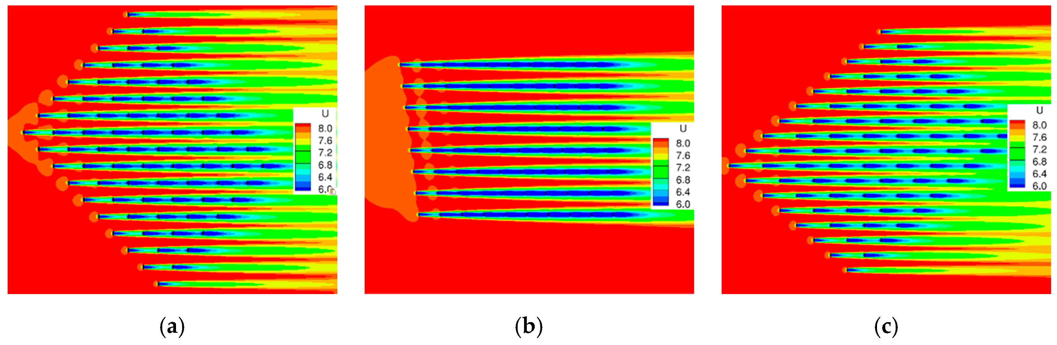Figure 10 displays the predicted axial velocity distribution at the hub height for various wind directions. The airflow obviously decelerates across wind turbines and the wake gradually recovers its velocity along the downstream direction. A slow wake recovery was found as airflow passes through multiple wind turbines. It is mainly due to a successive energy transfer from airflow to the wind turbine that results in less chance for airflow to receive energy from neighboring high velocity streams. The normalized power of a turbine row ($P_n)$ is defined as follows:

$$P_n=\frac{P_R}{P_1},$$

(19)

where $P_1$ represents the power of the first wind turbine row and $P_R$ the power of a wind turbine row defined in Figure 8. The normalized power $P_n$ for three wind directions is forecasted in Figure 10, where the field measurement is labeled an average value alongside its upper and lower limits. For understanding the relative prediction accuracy of the proposed approach compared to other numerical approaches, a benchmark LES result [25] was chosen in this study to serve as a comparison basis of the numerical predictions. Figure 11 depicts the power forecast of the full model along with the LES prediction. In the case of $\alpha =220°$, the prediction of the full model favorably falls within the measurement limits. Despite a small overprediction of the average power output, the full model successfully delivered a sharp power drop in the second row, accompanied by a very mild power decrease along the downstream direction that truthfully describes the field performance of wind turbine rows. By contrast, the LES approach delivers a similar conclusion to the full model but it suggests an almost unchanged power tendency of the downstream rows where the average power is underpredicted especially for the second and third rows. For the wind farm simulation of $\alpha =270°$, the power forecast of the full model very well agreed with the measurement, except for a within-limits overprediction of the average power at the second row, whereas the LES prediction gives an obvious underprediction for all downstream wind turbine rows in addition to a deep power deficiency of the second row that is apparently inconsistent with the wind farm measurement. A large discrepancy between the measurement and the numerical result predicted by the full model, as well as the LES approach, was found in the power prediction of $\alpha =312°$. The field data indicates a clear power decline growing with the increase of the row number that is unable to be reproduced by both numerical approaches. One cause of this large disagreement on the power prediction might come to the unsatisfactory modeling of the turbulence development in the atmosphere boundary by both methods. As the tower spacing increases, the wake recovery is expected to become more pronounced. The nonlinear behavior of strong wake recovery at large tower spacing should be further investigated in future studies to obtain an accurate power prediction of wind turbine array, especially for the wind farms employing high-power wind turbines. Another reason for this substantial underprediction is the experimental data representing a period of measurement that records the wind turbine power under time-varying wind direction and speed rather than a fixed wind direction and speed in the ideal case considered in the numerical calculation. From this viewpoint, the case of $\alpha =222°$ clearly exhibits a more stable wind condition than the case of $\alpha =312°$. Figure 11 also compares the numerical results between the full and reduced models. Interestingly, the reduced model gives a very close result to the full model. This implies a significant reduction up to one order of magnitude in the computation cost can be easily achieved by utilizing the geographical symmetry without bring substantial modeling errors.

4.2. Long-Term Power Prediction

The power captured by a wind turbine mainly depends on its local wind conditions [26]. Hence, the long-years SCADA measurement was adopted to describe the local wind conditions. The SCADA data, such as wind velocity, wind direction, and power output, used in this study is recorded on a ten-minutes basis. However, these data possibly contain incomplete or erroneous information when the wind turbine is under maintenance, limits its power output, or experiences a system failure. Therefore, pre-processing is required to remove the invalid information inconsistent with the design power curve. Power prediction of a wind farm is an essential target of this study. However, wind velocity and wind direction randomly change in real wind conditions. In the long-term power prediction, to model wind conditions with high data frequency, do provide good time accuracy in power, but it is very time-consuming as well as computationally expensive. Hence, it is necessary to use a more robust and efficient approach to long-term power prediction. With a statistical analysis of the wind condition and its corresponding wind turbine power, a number of characteristic wind conditions, i.e., inflow wind direction and inflow wind velocity, were first defined for the wind farm under investigation. The power output of each characteristic wind condition was then predicted through a numerical simulation of the proposed actuator disk model. A power matrix to define the wind turbine power under the selected combination of inflow direction and inflow velocity was then obtained for the investigated wind turbine, Figure 12a, where α is the inflow direction, $U_{\mathrm{in}}$ the inflow velocity and P the power output of a wind turbine. The long-term power output of a wind turbine is therefore easily calculated via a numerical interpolation within the power matrix for any given wind condition. In regard to the accuracy of power prediction via the power matrix, a sufficient number of wind directions and wind velocities is generally required to satisfactorily resolve the meteorological features of the wind farm under investigation. In this study, 36 wind directions alongside 18 wind speeds were employed to defined the characteristic wind conditions. For the yearly SCADA data set with a data frequency of 10-min mean, the simulation cases were reduced from 52,560 to 648, namely a computation reduction in two orders of magnitude. For the onshore wind farms surveyed in this study and other similar wind farms where no anemometer is available to provide relevant atmospheric information for the power prediction, the wind condition had to be determined from the available SCADA data of the installed wind turbines. Because each wind turbine records the wind velocity and wind direction that it experiences, it is necessary to select a virtual anemometer independent of wind turbine locations for representing a unified and reasonable inflow condition for the wind farm. The inflow wind direction of a wind farm for a given time span is defined as the average wind direction of all wind turbines in the wind farm at that time span, Figure 12b:

$$\alpha =\frac{{\displaystyle {\sum }_{i=1}^{i=m}}{\alpha }_i}{m}$$

(20)

where $m$ denotes the total number of wind turbines installed in the wind farm. The inflow wind velocity is defined as the wind velocity recorded at the most upstream wind turbine with respect to the given inflow wind direction. Figure 12c schematically illustrates a wind farm with an inflow wind direction of 45°. In this case, the wind turbine WT2 is most upstream, so its wind velocity measurement was regarded as the inflow wind velocity of the wind farm for an inflow wind direction of 45°. Figure 13 shows the procedure for long-term wind farm power prediction. In this study, the capacity factor (CF) that represents the efficiency of a wind turbine over a time span is defined in Equation (21), where $t$ is the time span of interest and $P_r$ the rated power of the wind turbine studied.

$$\mathrm{CF}=\frac{1}{T}\frac{\int Pdt}{P_r}.$$

(21)

4.3. Description of Onshore Wind Farms

Three Taiwanese wind farms, labelled A, B, and C, were investigated for their long-term power prediction in this study. Wind farm A and wind farm B are onshore wind farms where the wind turbines reside along the coastline, while wind farm C is situated about 2 km away from a river mouth to the sea. The time span of SCADA data employed in this study for fixing the wind conditions was 54 months for wind farm A and 12 months for wind farms B and C. Figure 14 discloses the layouts of their wind turbine array, with the numbering of installed turbines where the direction of north is given in the upper right corner. Wind farm A has a wind turbine array of 8 Enercon E40-600 wind turbines. Figure 15a gives the power curve of the E40-600 wind turbine. The 600-kW wind turbine operates between a cut-in wind speed of 2.5 m/s and a cut-off wind speed of 25 m/s and has a rated wind speed of 13 m/s. The rotor speed of this wind turbine varies in the range of 18 rpm and 34.5 rpm. The wind conditions disclosed by SCADA are given in Figure 5b,c where ${\Phi }_{\mathrm{p}}$ denotes the probability function. The main wind direction of the wind farm A lies between $\alpha =20°$ and $35°$, while a probability peak around 17% occurs around a wind speed of 5 m/s. Ten Enercon E70 wind turbines builds the wind turbine array of wind farm B. The power characteristics of the Enercon E70 wind turbine are shown in Figure 16a, where the rated power of 2.3 MW is achieved at the rated wind speed of 15 m/s. This wind turbine starts to rotate at a wind speed of 2.5 m/s and stops to operate at a wind speed of 34 m/s. The allowable range of rotor speeds is designated between 6 rpm and 21.5 rpm. Figure 16b displays the wind direction experienced by the wind turbine WT1, which is the only available SCADA data for the wind direction in wind farm B. As indicated by this figure, the major wind direction is between 1$5°$ and $20°$. The maximum probability of the wind speed for wind farm B is about 11%, and the corresponding wind speed is approximately 3 m/s (Figure 16c). Wind farm C is the largest wind farm in wind turbine number, as well as in total power, compared to its two counterparts. There are 23 wind Vestas V80 turbines in total installed in wind farm C, which is designed in a two-row arrangement. The installed wind turbine features a rated power of 2 MW, a rated wind speed of 14.5 m, and a rated rotor speed of 16.7 rpm. The lower and upper limits of wind speed for a normal wind turbine operation are 3.5 m/s and 25 m/s, respectively. Figure 1a illustrates the power dependence on the wind speed of V80. Unlike the other two wind farms, wind farm C shows some disagreement in the wind direction among its wind turbines (Figure 17). This inconsistency in the wind direction was then technically removed in the statistical analysis in determining the inflow condition of a virtual anemometer, as described in the previous sections. The dominant wind direction nearly comes from the north with a variation of about 1$0°$. In contrast to the wind direction, the wind velocity exhibits a high consistence among wind turbines. A probability of 13% was found for a wind speed of 3 m/s (Figure 18). Clearly, wind farm A seems to have better wind conditions than wind farm B and wind farm C. The superior wind condition of wind farm A comes from its geographical advantage, i.e., a wind turbine array on an island in the Taiwan strait.

Table 5. Main parameters of the wind turbines installed at the investigated wind farms.

Wind Farm	Type	${\mathit{N}}_{\mathit{W}\mathit{T}}$	${\mathit{P}}_{\mathit{r}}\left(\mathbf{MW}\right)$	$\mathit{D}$	$\mathit{H}$	${\mathit{\omega }}_{\mathit{r}}\left(\mathbf{rpm}\right)$	${\mathit{U}}_{\mathit{r}}\left(\mathbf{m}\right)$
A	Enercon E40-600	8	0.6	40	46	34.5	13
B	Enercon E70	10	2.3	71	64	21.5	15
C	Vestas V80	23	2	80	70	16.7	14.5

summarizes the main geometry and operation parameters of the wind turbines installed at the wind farms investigated.

4.4. Yearly Capacity Factor

Figure 19a,b displays the wind conditions delivered by the virtual anemometer of wind farm A. These wind conditions indicate a dominant wind direction from the northeast in winter and from the southeast in the summer, while wind speed in the range between 5 m/s and 13 m/s has a probability function decreasing from 15% to 5%. Figure 19c shows the predicted yearly capacity factor for all wind turbines installed in wind farm A. The measurement indicates that the capacity factor of individual wind turbines varies between 0.4 and 0.46. The numerical prediction of the proposed approach delivers a mean capacity factor of 0.423 that well agrees with the measured b mean value of 0.432. The variation in CF among wind turbines seems to be underestimated by the numerical model, despite giving a similar tendency where the wind turbine WT6 delivers the least power among its counterparts. The power deficiency of WT6 can be explained by the high probability of the wind direction between $\alpha =15°$ and $25°$. As the wind condition falls in this range, WT6 directly suffers from the wake interaction with WT1 that accounts for its low capacity factor. The underestimation of the power variation in the wind turbine array should stem from the time resolution of SCADA data, i.e., a ten-minute mean. The averaging of wind speed and wind direction undoubtedly eliminate the power spike within a ten-minute time span, and hence lead to a smoother power history than instantaneous measurement. Figure 20a presents the wind velocity estimated by the virtual anemometer of wind farm B while the wind direction was already given in Figure 16b. The wind mainly comes from the northeast direction ($15°\le \alpha \le 20°$) in the cold season and from the southeast direction ($200°\le \alpha \le 210°$) in the hot season, together with the wind speed growing from 2.5 m/s to 15 m/s accompanied by a probability function falling from 8% to 3%. The estimated yearly capacity factor for all wind turbines installed in wind farm B is depicted in Figure 20b. The measured capacity factor of individual wind turbines oscillates between 0.3 and 0.39, whereas the numerical prediction shows a smaller range of power variation, $0.35\le \mathrm{CF}\le 0.39$. The predicted mean capacity factor, 0.38, favorably agrees with the measured mean capacity factor of 0.35. The overprediction, alongside a small power variation of the wind farm, as explained earlier, originates from the large time span of SCADA data. The improvement in predication accuracy requires us to use the wind conditions of smaller time intervals. Additionally, the proposed approach was unable to identify WT7 as a leading power contributor in the wind farm, and instead suggested an almost uniform power performance from WT1 to WT8, except for correctly recognizing WT9 and WT10 to be the least power contributors. The unsatisfactory prediction of power tendency among wind turbines is also heavily impacted by using a single wind turbine SCADA date to determine the incoming wind direction. Figure 20c unveils the major reason resulting in their power deficiency. Under the principal wind direction, i.e., $15°\le \alpha \le 20°$, WT9 and WT10 strongly suffers from a low incoming wind speed that clarifies their low mean value of the capacity factor. Figure 21a presents the dependence of the wind direction on its probability function, where the main wind direction resides in a region $0°\le \alpha \le 20°$. The maximum probability of 16% occurs at a wind speed of 5 m/s, while the probability function drops to 3% as the wind velocity reduces to the rated wind speed of 14.5 m/s, Figure 21b. The capacity factor for the wind turbines in wind farm C is compared between the numerical prediction and SCADA measurement in Figure 21c. The comparison shows that the measured capacity factor lies between 0.22 and 0.32, whereas the predicted capacity factor varies from 0.34 to 0.39. In respect to the wind farm power performance, the average capacity factor of the wind farm is 0.271 based on the SCADA data, whereas 0.368 is estimated by the numerical approach. A large discrepancy is apparently observed in the power prediction of wind farm C. Figure 21d shows a typical example of the raw SCADA data obtained from a wind turbine in wind farm C together with the design power curve. Noticeably, the real-time power is almost on the right-hand side of the design power curve. It implies a power degradation of deterioration of the wind turbine due to some unknown or unavailable reasons, because the design power curve generally serves as a mean line of the real-time power, as depicted in Figure 21e. This uncovers the main cause of large CF errors for wind farm C. A remedy is to obtain a corrected power curve based on the SCADA data to reflect the realistic power behavior of the wind turbine installed in the wind farm. The corrected power curve that truthfully delivers the correlation between the wind speed and the wind turbine power is given as the solid blue curve in Figure 21e. With this revision, the updated CF prediction is shown in Figure 21f, where the capacity factor of wind farm C is predicted to be 0.268. Nevertheless, the distinct CF variation among the installed wind turbines (~0.1) suggested by the SCADA data was unsurprisingly flattened into a much smaller value of 0.02, although the higher power output of the first-row turbines than the second-row turbines was still distinguishable from the numerical simulation.

Table 6. Comparison of yearly capacity factor among the investigated wind farms.

Wind Farm	$\mathit{A}$	$\mathit{B}$	$\mathit{C}$
CFE	0.432	0.350	0.271
CFS	0.423	0.380	0.268
Error (%)	2.1	8.6	1.1

shows a comparison of the yearly capacity factor of the investigated wind farms where the subscript S denotes the simulation result and the subscript E represents the SCADA measurement. The prediction error of the yearly capacity factor for a wind farm is less than 9% for a wind farm with a limited SCADA data set, whereas the prediction error can be reduced to 2% and less provided a more comprehensive SCADA data are available.

4.5. Performance Assessment of the Proposed Model

One important aim of this study is to establish a numerical model that can be easily applied in the early stages of wind farm development to verify or select an appropriate site for wind turbines in the planned wind farm, along with the capability to accurately estimate the long-term capacity factor required in financial investment in a wind farm project. To meet this target, a simplified nonlinear wake model based on the momentum theory is correspondingly proposed in this paper and an in-house code, WIFA3D, is accordingly implemented. Therefore, the momentum change of airflow across the wind turbine is directly governed by the power curve where no geometry details of blade section are required. In this way, the simplified actuator disk model can be directly used to verify the layout of a wind turbine array in the initial phase of a wind farm project when only the principal operation parameters, such as power curve and rotor speed, are available. Another advantage of this model is to offer sufficient prediction accuracy without demanding excessive computation expense. This model practically links the technical gap between the low-cost and less-accurate linear formulation and the high-cost and high-accuracy large eddy simulation. The prediction accuracy of the yearly capacity factor was clearly displayed in the cases of three onshore wind, where the individual prediction error ranged from 1.1% to 8.6% and the average prediction error was less than 4%. A recent study using the LES approach to validate the case of Horns Rev wind farm [27] was referenced to illustrate the computational benefit of the proposed approach. In the case of simulating a wind farm with eight cascading wind turbines, i.e., the reduced wind farm model with $\alpha =270°$, 6000 outer iterations are required by WIFA3D to achieve the numerical convergence. In the referenced LES study, 12,000 time steps for the wind farm simulation, alongside 200,000 time steps for the precursor computation, were reported with a comparable grid number. Because LES is a time-accurate computation, a converged solution of each time step commonly requires tens of outer iterations when the marching time step is moderate. Assuming that the computational cost of an outer iteration for both approaches to solve single scalar governing equation is approximately equal, the typical LES approach demands a computation cost about two orders of magnitude higher than the proposed approach. This highlights the computational efficiency of the proposed model. Despite delivering good prediction accuracy with low computation expense, the simplified actuator disk model has the following drawbacks. First, the proposed model shows a good prediction performance in the mean power, but it is prone to smooth the power variation among wind turbines in the same wind farm due to an averaging process in time and space. Second, the dynamic effect of power fluctuation contributed by the moving rotor, as well as by the unsteady incoming wind, is also unable to be reflected in its steady nature. Third, the uniform body force distribution based on the momentum conservation applied to the actuator disk could bring unfavorable impacts to the near wake because of the negligence of the blade aerodynamics. These issues also form the limitations of the proposed approach.

5. Conclusions

To meet the demand bridging the gap between low-cost linear formulation with unsatisfactory accuracy and the high-accuracy nonlinear models, such as large eddy simulation, featuring excessive computational costs, a simplified nonlinear wake model based on the momentum theory is proposed in this study to offer a reasonable balance between accuracy requirements and numerical expense. The numerical robustness of the proposed model further enables the establishment of an economic approach for long-term wind farm power prediction that provides the required information for the financial evaluation of wind farm development. The proposed model was first validated with the offshore measurement of Horns Rev wind farm for a given wind speed of 8 m/s alongside three wind directions. Except for the wind direction of 312°, the proposed approach delivered good agreement with the measurements, as well as a comparable accuracy level to the LES results. The in-house code WIFA3D only requires about one percent of the computational cost of the LES approach to predict the mean power delivered by a wind farm. This study also verifies that a reduced computational domain based on the symmetry of wind turbine arrays gives a significant computational advantage without sacrificing the prediction accuracy. This paper also proposes an efficient approach to predict the yearly capacity factor based on the characteristic wind conditions, where the required computational cost is possibly reduced by two orders of magnitude when compared with the traditional serial approach. The proposed approach can favorably forecast the yearly capacity factor of a wind farm with an average error of less than 5%, but the power variation across the wind turbine array is inevitably smoothed due to an averaging nature in time and space. The advantage of the simplified actuator disk model is demonstrated in its numerical robustness, as well as in the prediction accuracy of the mean power, whereas the time-accurate power behavior and the significant power variation among the wind turbines is unable to be captured by the proposed model due to its steady nature.

References

1. Skamarock, W.C.; Klemp, J.B.; Dudhia, J.; Gill, D.O.; Barker, D.; Duda, M.G.; Huang, X.; Wang, W.; Powers, J.G. A Description of the Advanced Research WRF Version 3 (No. NCAR/TN-475+STR); University Corporation for Atmospheric Research: Boulder, CO, USA, 2008. [Google Scholar]
2. Powers, J.G.; Klemp, J.B.; Skamarock, W.C.; Davis, C.A.; Dudhia, J.; Gill, D.O.; Coen, J.L.; Gochis, D.J.; Ahmadov, R.; Peckham, S.E.; et al. The Weather Research and Forecasting Model: Overview, System Efforts, and Future Directions. Bulletin Am. Meteorol. Soc. 2017, 98, 1717–1737. [Google Scholar] [CrossRef]
3. Mahoney, W.P.; Parks, K.; Wiener, G.; Liu, Y.B.; Myers, W.L.; Sun, J.; Monache, L.D.; Hopson, T.; Johnson, D.; Haupt, S.E. A Wind Power Forecasting System to Optimize Grid Integration. IEEE Trans. Sustain. Energy 2012, 3, 670–682. [Google Scholar] [CrossRef]
4. Haupt, S.E.; Mahoney, W.P. Taming Wind Power with Better Forecasts. IEEE Trans. Spectr. 2015, 52, 47–52. [Google Scholar] [CrossRef]
5. Ainslie, J.F. Calculating the Flow Field in the Wake of Wind Turbines. J. Wind Eng. Ind. Aerodyn. 1988, 27, 213–224. [Google Scholar] [CrossRef]
6. Sørensen, J.N.; Shen, W.Z. Numerical Modeling of Wind Turbine Wakes. J. Fluids Eng. 2002, 124, 393–399. [Google Scholar] [CrossRef]
7. González-Longatt, F.; Wall, P.; Terzija, V. Wake Effect in Wind Farm Performance: Steady-State and Dynamic Behavior. Renew. Energy 2012, 39, 329–338. [Google Scholar] [CrossRef]
8. Lin, Y.; Lee, N.Z.; Chau, S.W. Flow-Structure Interaction Modelling of Rotating Wind Turbine with Deformable Rotor Blades. In Proceedings of the 9th International Workshop on Ship and Marine Hydrodynamics, Glasgow, UK, 24–26 August 2015. [Google Scholar]
9. Chuang, Y.H.; Chau, S.W. Aerodynamic and Aeroacoustic Prediction of Wind Turbine Rotor for a 2MW Horizontal-Axis Design under the Rated Condition. In Proceedings of the 6th International Symposium on Energy Challenges and Mechanics, Inverness, Scotland, 14–18 August 2016. [Google Scholar]
10. Yang, C.Y.; Kouh, J.S.; Chau, S.W. Study of Aerodynamic Loads Acting on Wind Turbines under the Typhoon Conditions in Taiwan. In Proceedings of the Advanced Maritime Engineering Conference, Hong Kong, China, 13–14 October 2016. [Google Scholar]
11. Choi, N.J.; Nam, S.H.; Jeong, J.H.; Kim, K.C. Numerical Study on the Horizontal Axis Turbines Arrangement in a Wind Farm: Effect of Separation Distance on the Turbine Aerodynamic Power Output. J. Wind Eng. Ind. Aerodyn. 2013, 117, 11–17. [Google Scholar] [CrossRef]
12. Troldborg, N. Actuator Line Modeling of Wind Turbine Wakes. Ph.D. Thesis, Technical University of Denmark, Kongens Lyngby, Denmark, 2008. [Google Scholar]
13. Sørensen, J.N.; Mikkelsen, R.F.; Henningson, D.S.; Ivanell, S.; Sarmast, S.; Andersen, S.J. Simulation of Wind Turbine Wakes Using the Actuator Line. Tech. Phil. Trans. R. Soc. A 2015, 373, 20140071. [Google Scholar] [CrossRef] [PubMed] [Green Version]
14. Lanzafame, R.; Messina, M. Fluid Dynamics Wind Turbine Design: Critical Analysis, Optimization and Application of BEM Theory. Renew. Energy 2007, 32, 2291–2305. [Google Scholar] [CrossRef]
15. Porte-Agel, F.; Wu, Y.T.; Lu, H.; Conzemius, R.J. Large-eddy Simulation of Atmospheric Boundary Layer Flow through Wind Turbines and Wind Farms. J. Wind Eng. Ind. Aerodyn. 2011, 99, 154–168. [Google Scholar] [CrossRef]
16. Jha, P.K.; Churchfield, M.J.; Moriarty, P.J.; Schmitz, S. Guidelines for Volume Force Distributions within Actuator Line Modeling of Wind Turbines on Large-Eddy Simulation-Type Grids. J. Sol. Energy Eng. 2014, 136, 031003. [Google Scholar] [CrossRef]
17. Launder, B.E.; Spalding, D.B. Numerical Computation of Turbulent Flows. Comput. Methods Appl. Mech. Eng. 1974, 3, 269–289. [Google Scholar] [CrossRef]
18. Mikkelsen, R.F.; Sørensen, J.N. Actuator Disc Methods Applied to Wind Turbines. Doctoral Dissertation, Technical University of Denmark, Kongens Lyngby, Denmark, 2004. [Google Scholar]
19. Lee, K.C.; Chau, S.W. Wind Farm Wake Modeling Using an Actuator Disk Model. In Proceedings of the Advanced Maritime Engineering Conference, 9–12 October 2018. [Google Scholar]
20. Crasto, G.; Gravdahl, A.R.; Castellani, F.; Piccioni, E. Wake Modeling with the Actuator Disc Concept. Energy Procedia 2012, 24, 385–392. [Google Scholar] [CrossRef] [Green Version]
21. Castellani, F.; Vignaroli, A. An Application of the Actuator Disc Model for Wind Turbine Wakes Calculations. Appl. Energy 2013, 101, 432–440. [Google Scholar] [CrossRef]
22. Chau, S.W.; Hsu, K.L. Modeling Steady Axis-Symmetric Thermal Plasma Flow of Air by a Parallelized Magneto-Hydrodynamic Flow Solver. Comput. Fluids 2011, 45, 109–115. [Google Scholar] [CrossRef]
23. Stone, H.L. Iterative Solution of Implicit Approximations of Multidimensional Partial Differential Equations. SIAM J. Numer. Anal. 1968, 5, 530–558. [Google Scholar] [CrossRef]
24. Hsu, S.A.; Meindl, E.A.; Gilhousen, D.B. Determining the Power-Law Wind-Profile Exponent under Near-Neutral Stability Conditions at Sea. J. Appl. Meteorol. 1994, 33, 757–765. [Google Scholar] [CrossRef] [Green Version]
25. Wu, Y.T.; Porté-Agel, F. Modeling Turbine Wakes and Power Losses within a Wind Farm Using LES: An Application to the Horns Rev Offshore Wind Farm. Renew. Energy 2015, 75, 945–955. [Google Scholar] [CrossRef]
26. Jamil, M.; Parsa, S.; Majidi, M. Wind Power Statistics and an Evaluation of Wind Energy Density. Renew. Energy 1995, 6, 623–628. [Google Scholar] [CrossRef]
27. Dekos, G.; Piggot, M.D.; Laizet, S. Development and Validation of the High-Order Finite Difference Wind Farm Simulator, WInc3D. In Proceedings of the Third Conference on Renewable Energies Offshore, Lisbon, Portugal, 8–10 October 2018. [Google Scholar]
Figure 1. Wind turbine V80: (a) Power curve; (b) the correlation among U A V E , ω and P .
Jmse 08 00610 g001
Figure 2. (a) The arrangement of disk elements; (b) to distribute body force from a disk element to neighboring Cartesian cells.
Jmse 08 00610 g002
Figure 3. The solution procedure of the proposed numerical method.
Jmse 08 00610 g003
Figure 4. Computational domain adopted in the wind farm prediction.
Jmse 08 00610 g004
Figure 5. A Cartesian grid schematically employed in the grid-dependent study: (a) front view; (b) side view.
Jmse 08 00610 g005
Figure 6. Grid dependency study: (a) U A V E ; (b) discretization error.
Jmse 08 00610 g006
Figure 7. Horns Rev wind farm: (a) definition of wind direction; (b) grid arrangement for α = 270 °
Jmse 08 00610 g007
Figure 8. The definition of a turbine row in the full model: (a) α = 222 ° ; (b) α = 270 ° ; (c) α = 312 ° .
Jmse 08 00610 g008
Figure 9. The definition of a turbine row in the reduced model: (a) α = 222 ° ; (b) α = 270 ° ; (c) α = 312 ° .
Jmse 08 00610 g009
Figure 10. Axial velocity distribution at the hub height: (a) α = 222 ° ; (b) α = 270 ° ; (c) α = 312 ° .
Jmse 08 00610 g010
Figure 11. The comparison of power prediction: (a) α = 222 ° ; (b) α = 270 ° ; (c) α = 312 ° .
Jmse 08 00610 g011
Figure 12. (a) The power matrix of a wind turbine to define correlation among U in , α and P ; (b) the definition of inflow wind direction for a wind farm; (c) the wind farm with an inflow wind direction of 45 ° .
Jmse 08 00610 g012
Figure 13. The procedure for long-term wind farm power prediction.
Jmse 08 00610 g013
Figure 14. The wind turbine layout of the wind farm: (a) wind farm A; (b) wind farm B; (c) wind farm C.
Jmse 08 00610 g014
Figure 15. Wind farm A: (a) power curve; (b) wind direction probability; (c) wind velocity probability.
Jmse 08 00610 g015
Figure 16. Wind farm B: (a) power curve; (b) wind direction probability; (c) wind velocity probability.
Jmse 08 00610 g016
Figure 17. The wind direction probability of wind farm C: (a) Wind turbine (WT)1 to WT6; (b) WT7 to WT12; (c) WT13 to WT18; (d) WT19 to WT23.
Jmse 08 00610 g017
Figure 18. The wind velocity probability of wind farm C: (a) WT1 to WT12; (b) WT13 to WT23.
Jmse 08 00610 g018
Figure 19. Wind farm A: (a) wind direction probability; (b) wind velocity probability; (c) yearly capacity factor.
Jmse 08 00610 g019
Figure 20. Wind farm B: (a) wind velocity probability; (b) yearly capacity factor; (c) axial velocity distribution at the hub height for α = 20 ° and U in = 10 m/s.
Jmse 08 00610 g020
Figure 21. Wind farm C: (a) wind direction probability; (b) wind velocity probability; (c) yearly capacity factor; (d) power curve; (e) corrected power curve; (f) yearly capacity factor with the corrected power curve.
Jmse 08 00610 g021