Article

Improvement of the Full-Range Equation for Wave Boundary Layer Thickness

1
Department of Civil Engineering, Tohoku University, 6-6-06, Aoba, Sendai 980-8579, Japan
2
Department of Civil Engineering and Architecture, Sultan Qaboos University, P.O. Box 33, 123 Al-Khoud, Muscat, Sultanate of Oman
*
Author to whom correspondence should be addressed.
J. Mar. Sci. Eng. 2020, 8(8), 573; https://doi.org/10.3390/jmse8080573
Submission received: 7 July 2020 / Revised: 27 July 2020 / Accepted: 28 July 2020 / Published: 30 July 2020

Abstract

:
In order to improve the accuracy of the original full-range equation for wave boundary layer thickness, with special reference to increasing its applicability to tsunami-scale waves, a theoretical investigation is carried out to derive a dimensionless expression which is valid under both smooth and rough turbulent regimes. A coefficient in the equation is determined through a comparison with k- ω  model computation results for tsunami-waves along with laboratory scale oscillatory flow experiments. Thus, the improved full-range equation for wave boundary layer thickness enables us to cover a wide range of wave periods from wind-wave to tsunami.

1. Introduction

The 2011 Tohoku tsunami caused highly devastating disasters to human lives, infrastructure, and coastlines in the north-eastern region of Japan. The extreme tsunami-induced flow velocity caused remarkable morphology change in coastal and estuarine areas in Tohoku region. Using highly valuable field data of morphology changes [1,2], many researches have been able to calibrate and validate a numerical model for tsunami-induced sediment transport and resulting morphology change [3,4]. In these numerical investigations, it is common to use a steady friction factor for estimating bottom shear stress under tsunami. However, according to a numerical study using k- ω turbulence model by Williams and Fuhrman [5], tsunami-induced boundary layer is wave-like in the sense that the boundary layer does not necessarily span the entirety of the water depth. In addition, a recent field investigation during the 2010 Chilean tsunami revealed that the velocity profile at a water depth of 10 m is extremely similar to that under wave motion with very thin boundary layer thickness [6]. Tinh and Tanaka [7] reported that the ratio of δ / h ( δ : the wave boundary layer thickness under tsunami, h : the water depth) is suitable for judging whether a tsunami-induced boundary layer is wave-like or current-like.
Wave boundary layer thickness has been formulated mainly using experimental results obtained in an oscillating tunnel [8,9,10,11]. It is well known that laminar wave boundary layer thickness is proportional to ( ν T ) 1 / 2 ( ν : kinematic viscosity, T : wave period) according to Stokes second problem [12]. Thus, the boundary layer thickness developed in a wave flume is rather small (order of 0.1 cm). For this reason, a closed type of oscillating tunnel has been developed [13] to increase the period of oscillatory motion, and has been extensively applied by many researchers for studying various topics related to wave motion including boundary layer structure, sediment movement, and force acting on coastal structures under oscillatory motion [14,15,16,17].
Nonetheless, the period of the oscillatory motion in these experimental facilities is extremely smaller than that under tsunami. Tinh and Tanaka [7] carried out an investigation on the development of a bottom boundary layer under shoaling tsunami using the formula proposed by Sana and Tanaka [11]. In their study, a hypothetical tsunami shoaling case was configured. Similar to Williams and Fuhrman [5], an initial offshore tsunami of 1 m high with the wave period 15 min at the water depth of 4000 m that propagates over 200 km to the shallow area is considered. As a result, it is shown that depth-limited condition, δ = h is not satisfied by tsunami boundary layer even at the water depth shallower than h = 10   m , which shows good agreement with the field measurement by Lacy and colleagues [6]. However, it is noted that the equation proposed by Sana and Tanaka [11] is applicable to wind-generated waves, and it is not clear whether it can be applied to long period wave by extrapolation. In the present study, therefore, a theoretical framework is developed for boundary thickness under turbulent conditions covering both wind-waves and tsunami. Furthermore, a semi-empirical formula is proposed for wave boundary layer thickness using laboratory data along with numerical results by k- ω turbulence model.

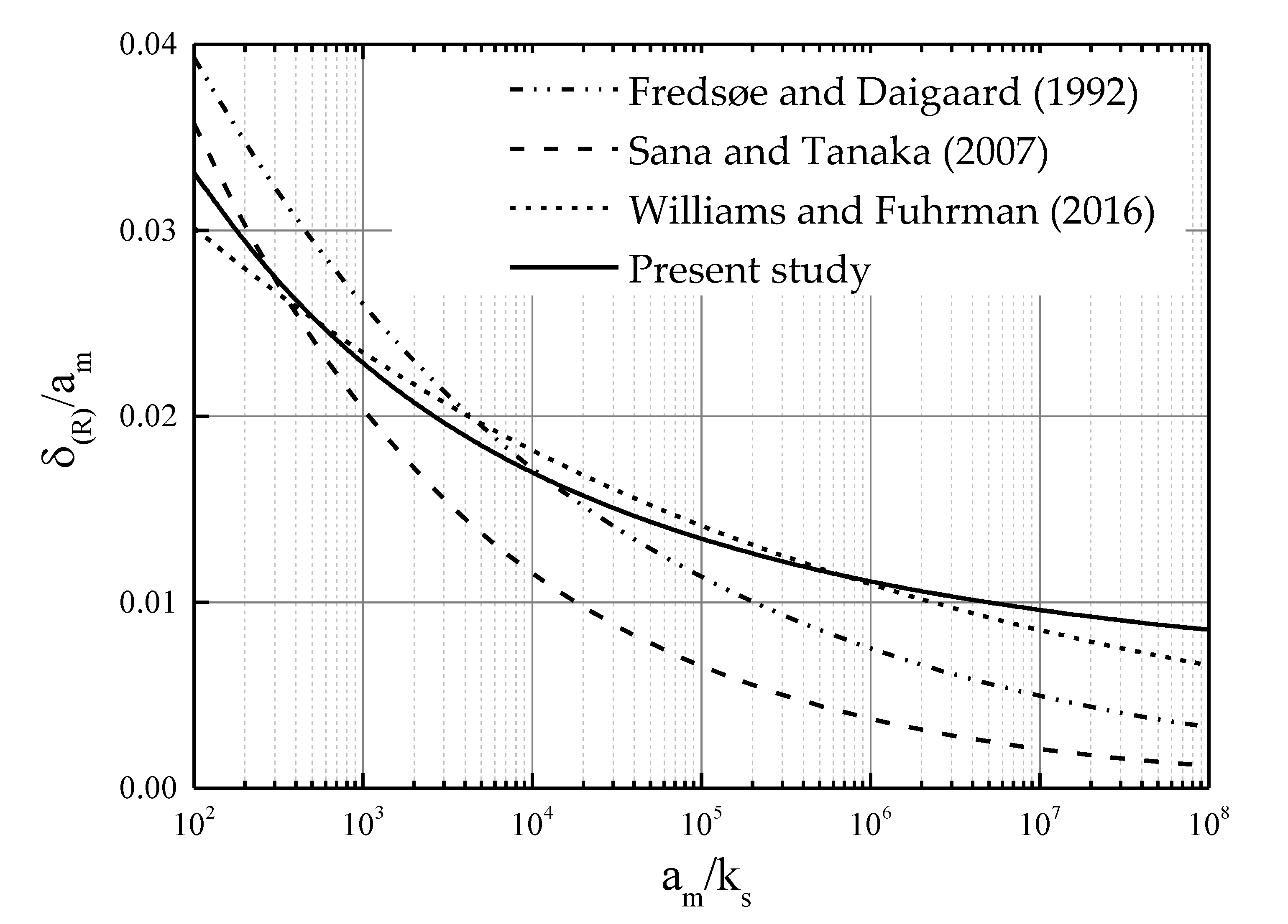
2. Comparison of Existing Formulae
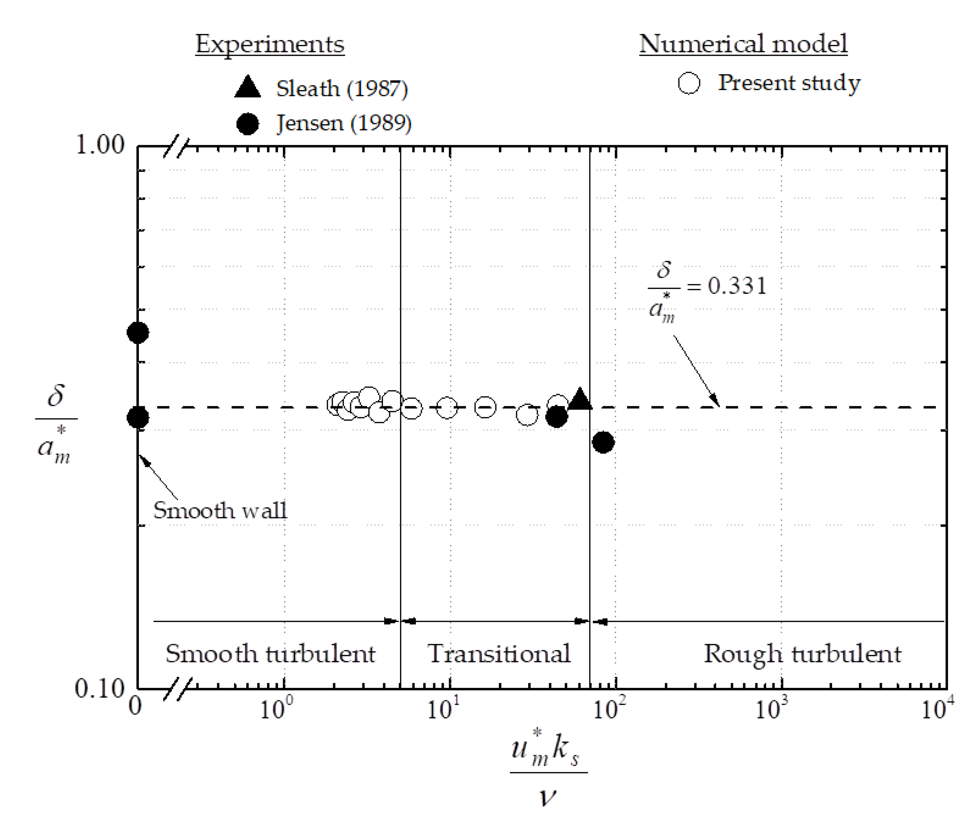
Our interest herein will be limited to the wave boundary layer under sinusoidal wave motion. In the case of the laminar boundary layer, the governing equation is given as follows.
u t = U t + ν 2 u z 2
where u : the horizontal velocity in the wave boundary layer, t : the time, U : the free stream velocity outside the boundary layer, and z : the vertical coordinate. In order to solve Equation (1), the following two boundary conditions are imposed.
u = 0 at z = 0
U = U m sin σ t at z =
where U m : the amplitude of U , and σ : the angular frequency (= 2 π / T ). From these equations, the following analytical solution can be obtained for the velocity distribution in a boundary layer [16].
u U m = sin σ t exp ( z δ 1 ) sin ( σ t z δ 1 )
where δ 1 : the Stokes layer thickness (= 2 ν / σ ). The time-variation of velocity distribution over a wave cycle from Equation (4) is shown in Figure 1. One of the important characteristics of the wave boundary layer is an overshoot phenomenon near the bottom as illustrated in Figure 1. Jensen et al. [9] defined the height of overshoot under the wave crest as a wave boundary layer thickness δ , and obtained the following analytical expression.
δ ( L ) a m = 3 π 4 ( 2 Re ) 1 / 2
where the subscript (L) denotes laminar condition, and Re in Equation (5) is Reynolds number defined by
Re = U m a m ν
in which am is the amplitude of water particle movement outside the wave boundary layer as
a m = U m σ
Alternative definitions for wave boundary layer thickness have been employed by other researchers, such as the minimum distance from the bottom to a point where the horizontal velocity equals free-stream wave velocity amplitude [16], and the elevation of 1% or 5% velocity deficit at the outer edge of the boundary layer [8,18]. Among these definitions, that of Jensen et al. [9] is the most suitable for the present study, since we will discuss the depth-limited condition of tsunami boundary layer, in which a shear-free condition needs to be exactly satisfied on the water surface.
According to Equation (5), it is easily shown that wave boundary layer thickness under laminar condition is proportional to ( ν T ) 1 / 2   as mentioned before.
At higher Reynolds numbers, transition to a turbulence occurs around Re = 2.5 × 10 5 [19,20]. Depending on different criteria for defining the transition, slightly different values have been proposed (see [21,22]). For turbulent regime, analytical solution cannot be obtained for boundary layer thickness. Hence, an empirical approach has been applied based on laboratory experiments or numerical analysis using a turbulence model such as k- ε model and k- ω model. The following equations have been proposed for smooth turbulent and rough turbulent conditions.
  • Smooth turbulent
    -
    Fredsøe and Daigaard [10]
    δ ( S ) a m = 0.086   Re 0.11
    -
    Sana and Tanaka [11]
    δ ( S ) a m = 0.017   Re 0.011
    -
    Williams and Fuhrman [5]
    δ ( S ) a m = 0.044   Re 0.07
  • Rough turbulent
    -
    Fredsøe and Daigaard [10]
    δ ( R ) a m = 0.09 ( a m k s ) 0.18
    -
    Sana and Tanaka [11]
    δ ( R ) a m = 0.111 ( a m k s ) 0.246
    -
    Williams and Fuhrman [5]
    δ ( R ) a m = 0.05 ( a m k s ) 0.11
where the subscripts (S) and (R) denote rough turbulent and smooth turbulent, respectively, and ks is the equivalent roughness. Among these, Williams and Fuhrman’s [5] equations have been proposed based on k- ω numerical simulation for tsunami-like long period waves.
Figure 2 shows comparison among Equations (8)–(10) for smooth turbulent condition. It is seen that Equations (8) and (10) have similar behavior, whereas the equation by Sana and Tanaka [11] has a smaller dependence on the Reynolds number. The line designated “Present study” represents a new equation proposed in this paper, which will be described later.
Similarly, Figure 3 shows comparison of three equations for boundary layer thickness under rough turbulent condition. Again, the equation proposed by Sana and Tanaka [11] differs distinctly from other equations especially at higher a m / k s due to its larger power in Equation (12), which may cause underestimation of the boundary layer thickness for tsunami waves with a longer wave period.
It must be stressed here that each empirical equation is applicable in the region of available data on which the equation is based. For this reason, applicability of equations needs to be carefully investigated when it is extrapolated to longer wave motion like tsunami.

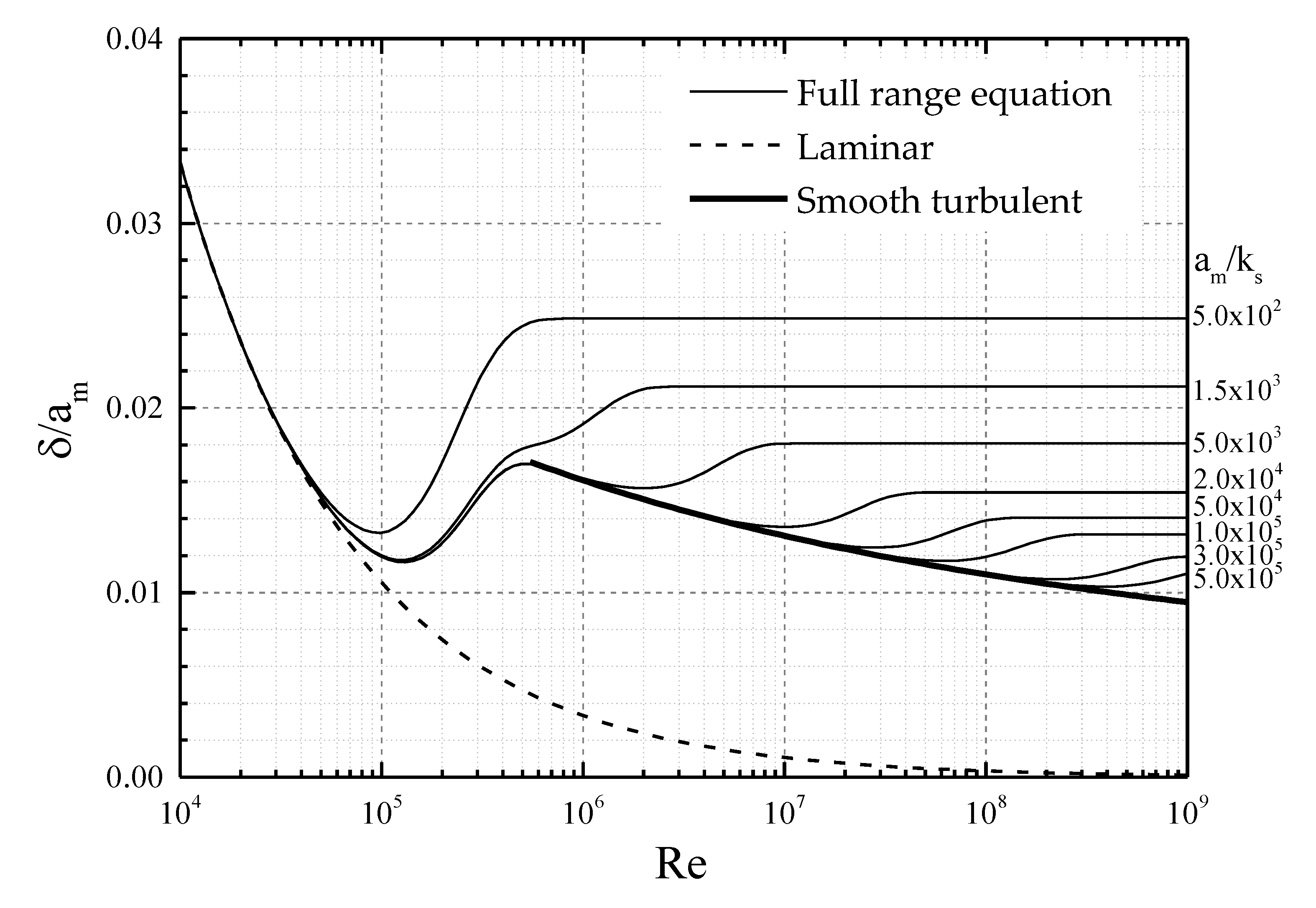
3. Proposal of New Formulae for Turbulent Flow

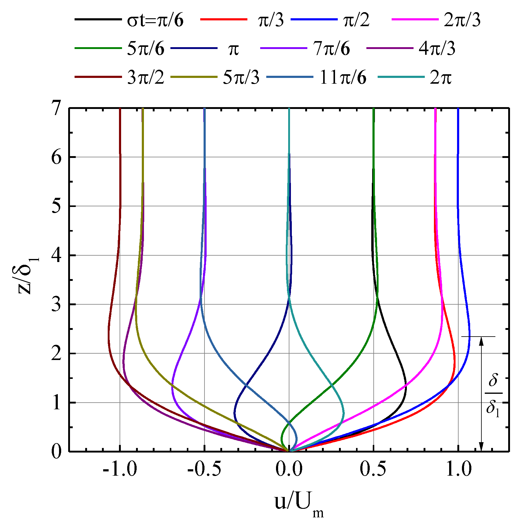
3.1. Theoretical Consideration

Hereafter, dimensionless expression will be derived for boundary layer thickness which is valid for both smooth turbulent and rough turbulent conditions.
As described above, the boundary layer thickness under laminar condition can be expressed as δ ( ν T ) 1 / 2 . This is a representative length common for various physical processes expressed in terms of the diffusion equation. For example, equivalent representative length can be derived in heat conduction theories [23], viscous fluid theories [12] and also in a shoreline change model based on a one-line model [24,25]. After transition to turbulence at higher Reynolds numbers, the molecular viscosity in the equation for wave boundary layer thickness might be replaced by eddy viscosity ν t . Kajiura [26] and Tanaka and Shuto [27] used the following assumption to derive an analytical solution for turbulent wave boundary layer.
ν t = κ u m * z
where κ : the Karman constant (=0.4), and u m * : the maximum friction velocity.
The dependence on z in Equation (14) is originated from mixing length, l = κ z , due to turbulent momentum transfer. Alternative assumption for wave-induced eddy viscosity may be constant expression, rather than spatially varying as Equation (14), as assumed by Kajiura [26] in the outer layer of the wave boundary layer. Then, replacing z in Equation (14) by δ , the following equation can easily be obtained for wave boundary layer thickness under turbulent conditions.
δ a m * = c o n s t .
where a m * is defined by
a m * = u m * σ = U m σ f w 2 = a m f w 2
where f w : the wave friction coefficient. Here, the relationship between a friction coefficient and friction velocity u m * is given by the following formula.
u m * = U m f w 2
It is interesting to note that the non-dimensional quantity defined by Equation (15) has already been used in theoretical study for turbulent wave boundary layer by Kajiura [26], Grant and Madsen [28], and Tanaka [29]. Another interesting point is mathematical similarity between laminar and turbulent flow in the denominator of the left-hand side of Equation (5), am, and the corresponding expression in Equation (15), a*m.
In order to validate Equation (15), velocity profile data under wave crest ( σ t = 0   deg) were collected as summarized in Table 1. In both laboratory experiments by Sleath [8] and Jensen [30], a U-shaped oscillating tunnel was used to obtain detailed velocity profile under oscillatory boundary layer. In addition to these two experimental results, k- ω turbulence modeling is conducted for tsunami wave boundary layer as listed in Table 1. These are hypothetical shoaling tsunami cases investigated by Tinh and Tanaka [7]. Figure 4 indicates conditions of the whole test cases summarized in Table 1. Most of the data have sufficiently high Reynolds number to fall in the turbulent regime. In addition, the present computational cases using k- ω model range from moderate to sufficiently high values of R e and a m / k s , due to an input of longer period of tsunami wave as seen in Table 1.
In the numerical computation of k- ω model, the boundary layer equation is solved by finite difference method using an implicit scheme [31]. Sufficiently fine mesh size is employed in the immediate vicinity of the bottom, with gradually increasing mesh spacing in the vertical upward direction [32].
Considering the dimensionless quantity defined in Equation (15), the whole data sets are plotted in Figure 5 and Figure 6 using the common vertical coordinate ζ.
ζ = z a m *
It is clearly observed in Figure 5 and Figure 6 that all data sets indicate overshooting velocity profile at ζ = 0.331 , below which the velocity reduces gradually following logarithmic law with different velocity gradient. In addition, it is evident that Jensen [30] and the present numerical simulations are more suitable for detecting the exact elevation of overshooting height due to their finer interval of measurements and simulations.
For further investigation on wave boundary layer thickness, the height of the overshooting from these data sources is plotted in Figure 7. The variable on the abscissa is the roughness Reynolds number which can be utilized for classifying the flow regime under turbulent conditions into smooth and rough as shown previously [20].
Smooth   bottom :   u m * k s ν < 5
Transition   region :   5 u m * k s ν 70
Rough   bottom :   u m * k s ν > 70
The data sets listed in Table 1 fully encompass smooth, transitional, and rough regimes (Figure 7). In addition, the constant defined in Equation (15) can be determined to be 0.331. Hence, we obtain the following equation, which is half theoretical and half empirical.
δ a m * = 0.331
It is important to note that in the theoretical treatment to derive Equation (22), the flow regime is assumed to be simply turbulent, and thus the classification into smooth and rough is not required. Hence it is concluded that Equation (22) is valid for both smooth and rough turbulent regimes. This is a distinct difference as compared with existing formulas from Equations (8)–(13).

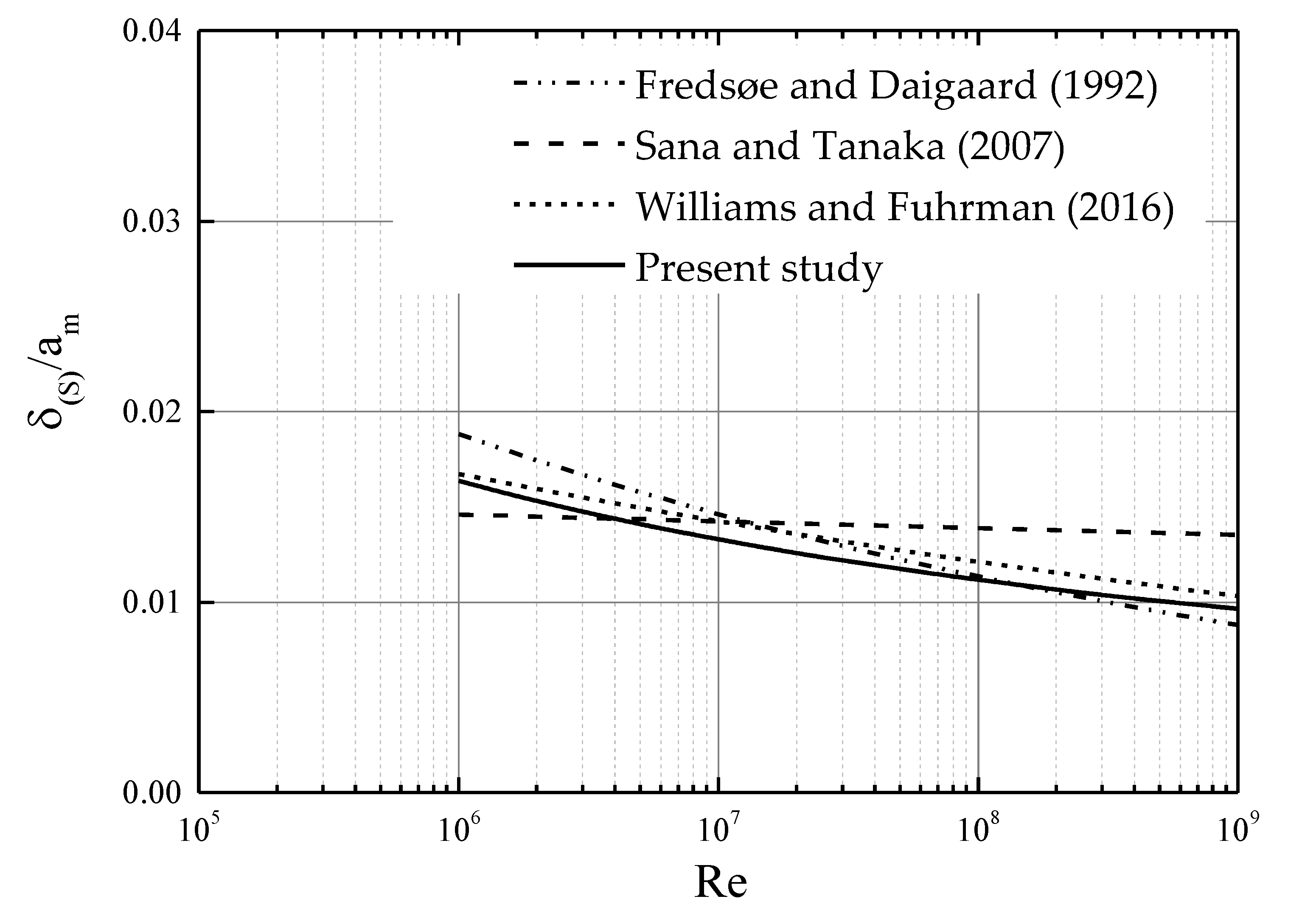
3.2. Proposal of New Calculation Formulas for Each Flow Regime

Although Equation (22) has superiority over the existing expressions in the sense that it is valid for a turbulent regime regardless of bottom roughness condition, its convenience in practical applications might be improved by deriving an equation for each flow regime expressed in terms of Re and a m / k s . Therefore, friction coefficient under wave motion can be substituted into Equation (22). Here the following explicit form of wave friction coefficient for smooth bottom [20] and rough bottom [33] proposed by the one of the authors is used.
f w ( S ) = exp { 7.94 + 7.35 Re 0.0748 }
f w ( R ) = exp { 7.53 + 8.07 ( 30 a m k s ) 0.100 }
By substituting these two friction factors into Equation (22), a convenient formula for wave boundary thickness can be obtained for smooth and rough turbulent flows separately.
δ ( S ) a m = 0.234 exp { 3.97 + 3.68 Re 0.0748 }
δ ( R ) a m = 0.234 e x p { 3.77 + 4.04 ( 30 a m k s ) 0.100 }
The equations obtained in the present study are illustrated in Figure 2 and Figure 3. In the range of higher Re and a m / k s corresponding to tsunami-scale wave motion, the present equations show good agreement with Williams and Fuhrman [5].

3.3. Full-Range Equation

Sana and Tanaka [11] proposed a full-range equation applicable to all flow regimes spanning laminar, smooth turbulent, and rough turbulent. However, it is shown in this study that the equations for smooth turbulent and rough turbulent proposed by Sana and Tanaka [11] need to be replaced by Equations (25) and (26), respectively, to be more accurate up to higher values of Re and a m / k s . Accordingly, computation method of δ for an arbitrary flow regime including transitional regime is as follows [11].
δ a m = f 2 { f 1 δ ( L ) a m + ( 1 f 1 ) δ ( S ) a m } + ( 1 f 2 ) δ ( R ) a m
where f 1 and f 2 are given by
f 1 = e x p { 0.941 ( Re 2.5 × 10 5 ) 2.01 }
f 2 = e x p { 0.0101 ( Re R 1 ) 2.06 }
in which R 1 is defined by
R 1 = 25 ( a m k s ) 1.15
In order to apply Equation (27), the expressions for each flow regime, Equations (5), (25), and (26), will be substituted, rather than Equations (9) and (12). The result obtained by the full-range equation is illustrated in Figure 8. It is seen that highly smooth transitional behavior can be obtained from Equation (27). However, as compared with the previous diagram proposed by Sana and Tanaka [11], the transition from laminar to smooth turbulent flow is more abrupt.
In recent years, experimental studies have been carried out for boundary layers in an acceleration-skewed oscillatory flow (e.g., Suntoyo et al. [17], van der A et al. [34], and Yuan and Wang [35]). The equations proposed herein for a sinusoidal motion can be applied to acceleration-skewed oscillatory waves as well by introducing an equivalent sinusoidal orbital amplitude, ac, for am as proposed by Suntoyo et al. [17] and van der A et al. [34].

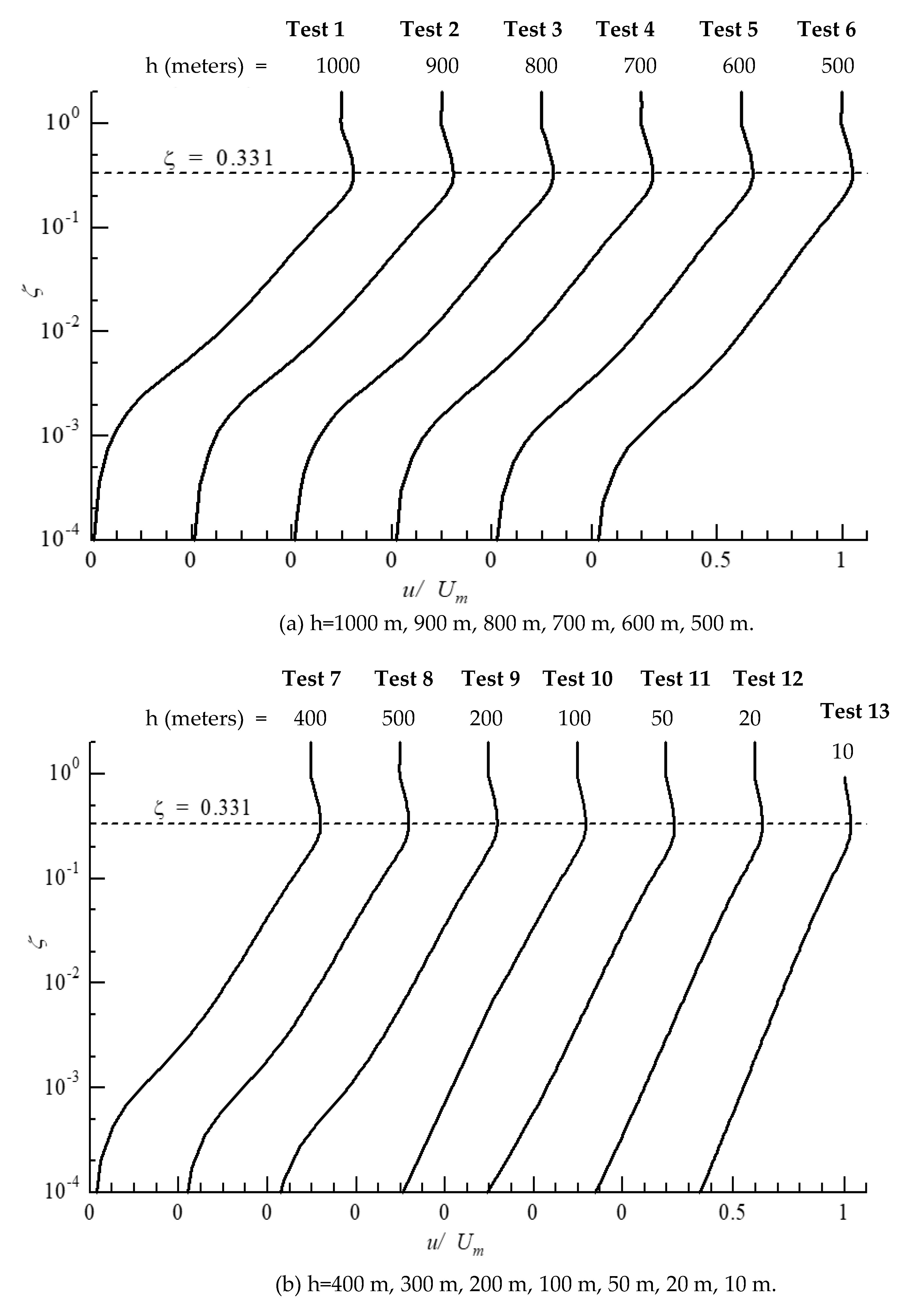
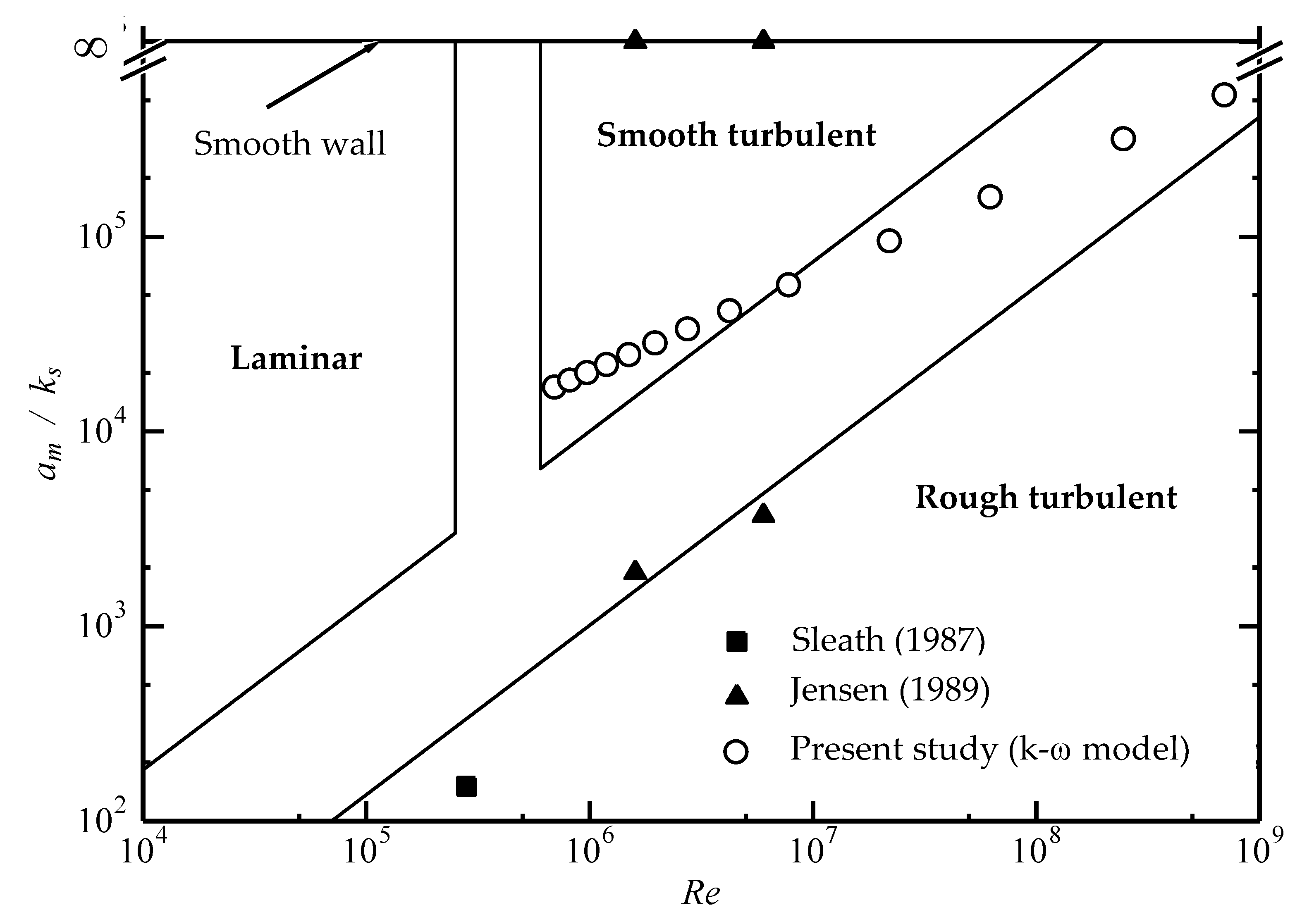
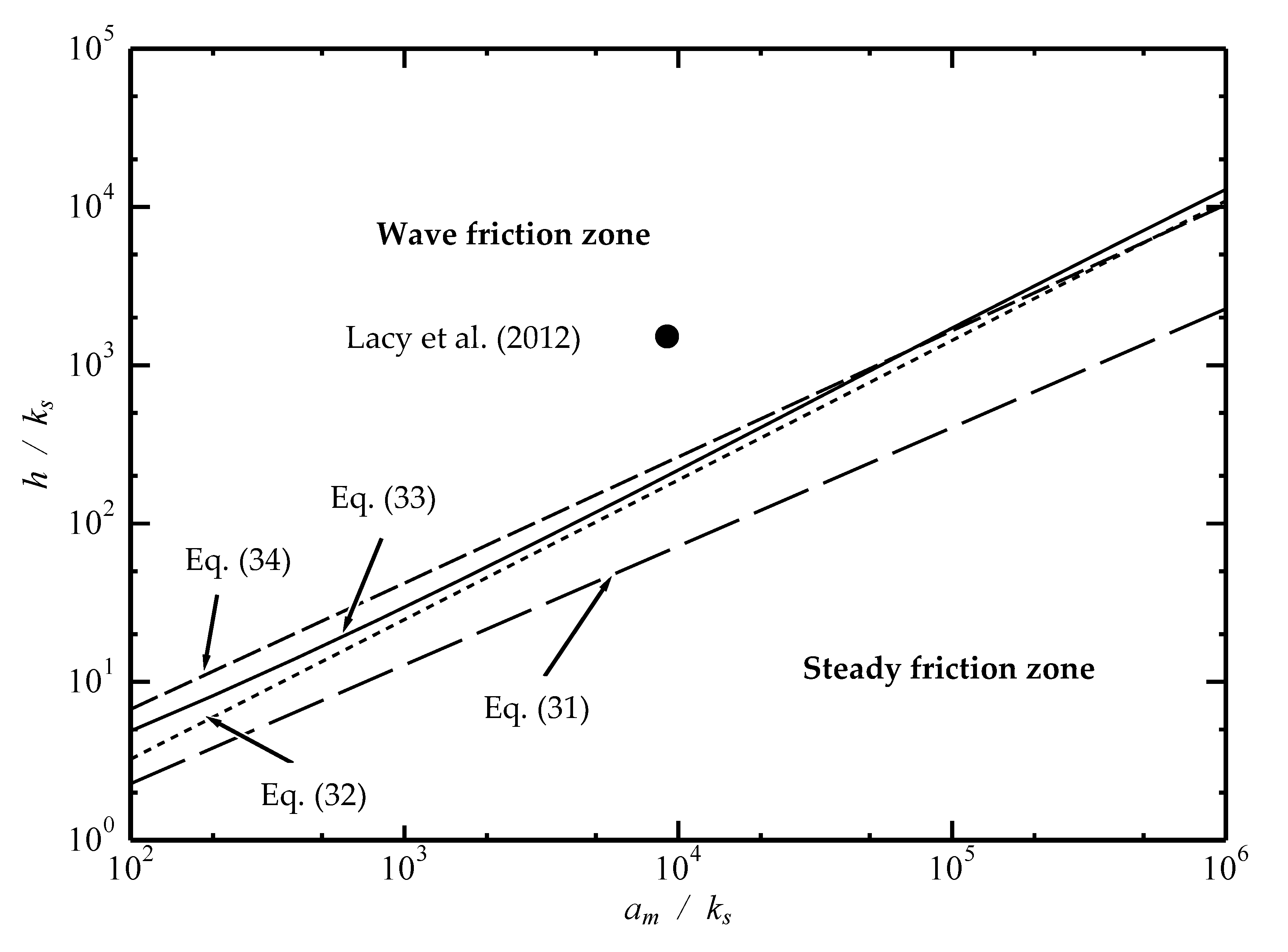
4. Application of the New Formula to Demarcation of Friction Law under Tsunami

Tinh and Tanaka [7] proposed equations and a diagram demarcating wave friction zone and steady friction zone under shoaling tsunami. Using Equation (12), Tinh and Tanaka [7] obtained the following criteria for demarcating friction laws by assuming h = δ .
h k s = 0.111 ( a m k s ) 0.754
Meanwhile, using the newly obtained equation for boundary layer thickness for rough turbulent regime, Equation (26), an alternative equation is obtained by assuming h = δ .
h k s = 0.234 a m k s exp { 3.77 + 4.04 ( 30 a m k s ) 0.100 }
By equating wave friction factor f w and steady current friction factor f c , Tinh and Tanaka [7] proposed a demarcation in terms of friction factor.
exp { 7.53 + 8.07 ( 30 a m k s ) 0.100 } = 2 κ 2 { ln ( 30 h k s ) 1 } 2
In addition, Tanaka et al. [36] empirically determined the following criterion for frictional factor demarcation under tsunami.
h k s = 0.171 ( a m k s ) 0.797
Equations (31)–(34) are plotted in Figure 9 for comparison. It is observed in Figure 9 that Equation (31) is very far from other criteria. However, by replacing the previous boundary layer thickness formula with the improved one, newly obtained criterion in terms of boundary layer thickness (Equation (32)) gives a result which is very close to Equations (33) and (34), especially at a higher value of a m / k s . It is interesting to note that the field data of Lacy et al. [6] during the 2010 Chilean tsunami can successfully be classified into the wave friction zone.
Since the equations proposed herein are based on linear wave theory, modification is required when we apply them to real tsunami events, in which wave motion is usually transient. Larsen and Fuhrman [37,38] proposed a method to use time-varying boundary layer thickness by replacing the orbital amplitude with the cumulative distance traveled by a free-stream particle.

5. Conclusions

In this study, investigation on wave boundary layer thickness was carried out, aiming to increase the applicability of the existing formulas to tsunami waves. According to comparisons among three existing formulas, it was found that Sana and Tanaka’s [11] equation gives different behavior as compared with others at higher Re and a m / k s . Therefore, a new calculation formula was proposed based on the theoretical consideration using an eddy viscosity coefficient. By applying newly obtained equations for smooth and rough turbulent regimes, a full-range equation was successfully reconstructed, which enabled us to calculate wave boundary layer thickness automatically without judgment of flow regime for a set of given input parameters. In addition, the new equation can be successfully applied for demarcating friction factor under tsunami. The findings of this study will improve the prediction of sediment movement under long waves by providing more accurate boundary layer thickness under variable field conditions.

Author Contributions

H.T. wrote most of the manuscript and contributed to the interpretation of the results. N.X.T. and A.S. performed the experimental data analysis and numerical simulation as well as prepared for the figures. All authors have read and agreed to the published version of the manuscript.

Funding

This research was funded by the Taisei Foundation.

Acknowledgments

The authors would like to express their sincere gratitude to the financial support from the Taisei Foundation.

Conflicts of Interest

The authors declare no conflict of interest.

References

  1. Tanaka, H.; Tinh, N.X.; Umeda, M.; Hirao, R.; Pradjoko, E.; Mano, A.; Udo, K. Coastal and Estuarine Morphology Changes Induced by the 2011 Great East Japan Earthquake Tsunami. Coast. Eng. J. 2012, 54, 1250010. [Google Scholar] [CrossRef]
  2. Tanaka, H.; Adityawan, M.B.; Mano, A. Morphological changes at the Nanakita River mouth after the Great East Japan Tsunami of 2011. Coast. Eng. 2014, 86, 14–26. [Google Scholar] [CrossRef] [Green Version]
  3. Sugawara, D.; Takahashi, T.; Imamura, F. Sediment Transport Due to the 2011 Tohoku-Oki Tsunami at Sendai: Results from Numerical Modeling. Mar. Geol. 2014, 358, 18–37. [Google Scholar] [CrossRef]
  4. Yamashita, K.; Sugawara, D.; Takahashi, T.; Imamura, F.; Saito, Y.; Imato, Y.; Kai, T. Numerical Simulations of Large-scale Sediment Transport Caused by the 2011 Tohoku Earthquake Tsunami in Hirota Bay, Southern Sanriku Coast. Coast. Eng. J. 2016, 58, 1640015. [Google Scholar] [CrossRef] [Green Version]
  5. Williams, I.A.; Fuhrman, D.R. Numerical simulation of tsunami-scale wave boundary layers. Coast. Eng. 2016, 110, 17–31. [Google Scholar] [CrossRef] [Green Version]
  6. Lacy, J.R.; Rubin, D.M.; Buscombe, D. Currents, drag, and sediment transport induced by a tsunami. J. Geophys. Res. 2012, 117, C9. [Google Scholar] [CrossRef]
  7. Tinh, N.X.; Tanaka, H. Study on boundary layer development and bottom shear stress beneath a tsunami. Coast. Eng. J. 2019, 61, 574–589. [Google Scholar] [CrossRef]
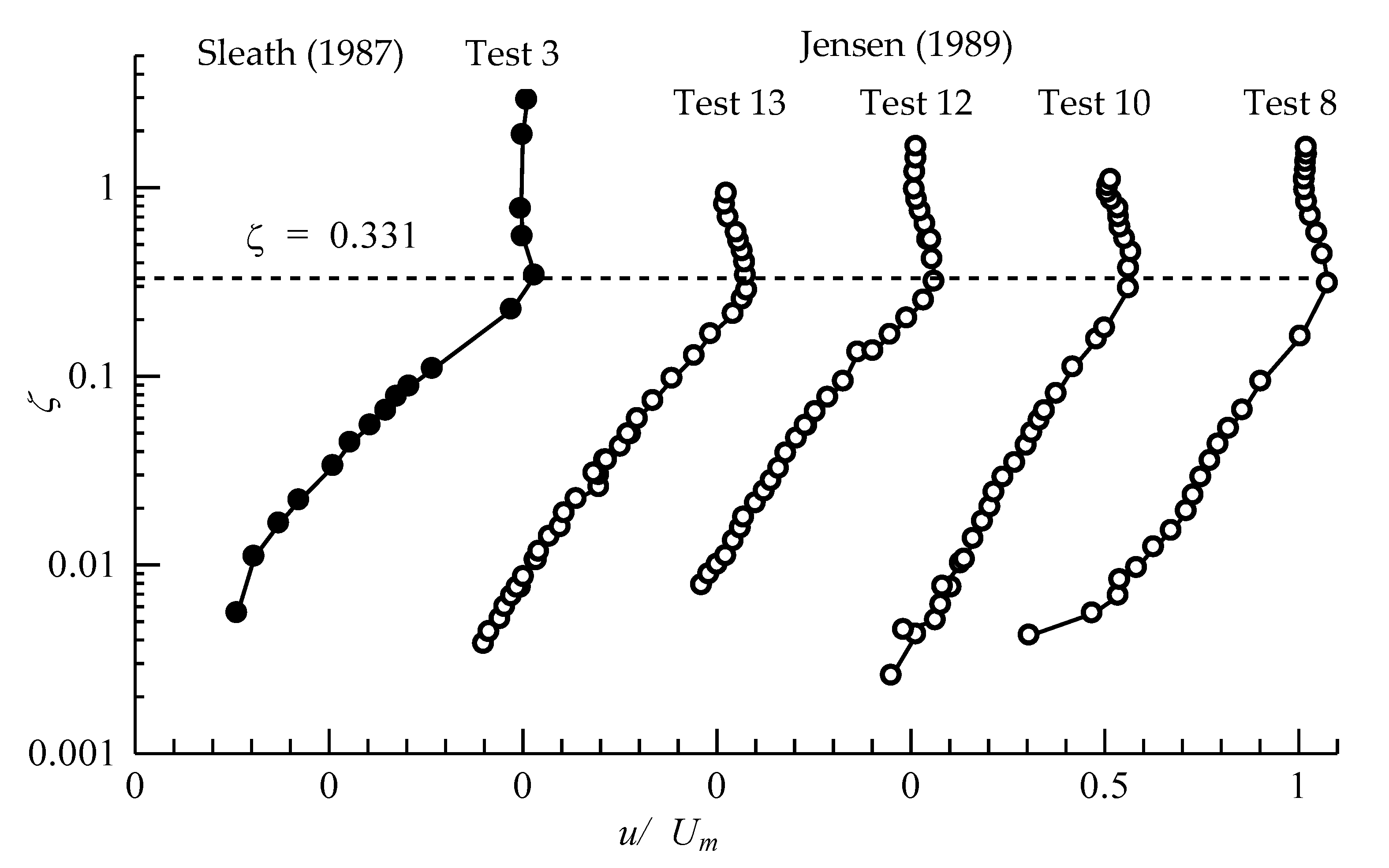
  8. Sleath, J.F.L. Turbulent oscillatory flow over rough beds. J. Fluid Mech. 1987, 82, 369–409. [Google Scholar] [CrossRef]
  9. Jensen, B.L.; Sumer, B.M.; Fredsøe, J. Turbulent oscillatory boundary layers at high Reynolds numbers. J. Fluid Mech. 1989, 206, 265–297. [Google Scholar] [CrossRef] [Green Version]
  10. Fredsøe, J.; Deigaard, R. Mechanics of Coastal Sediment Transport; World Scientific: Singapore, 1992; 369p. [Google Scholar]
  11. Sana, A.; Tanaka, H. Full-range equation for wave boundary layer thickness. Coast. Eng. 2007, 54, 639–642. [Google Scholar] [CrossRef]
  12. Schlichting, H. Boundary Layer Theory, 9th ed.; Springer: Berlin/Heidelberg, Germany, 1979; 805p. [Google Scholar]
  13. Lundgren, H.; Sorensen, T. A pulsating water tunnel. In Proceedings of the 6th International Conference on Coast. Eng., Gainesville, FL, USA, 29 January 1957; pp. 356–358. [Google Scholar]
  14. Kamphuis, J.W. Friction factor under oscillatory waves. J. Waterw. Port Coast. Ocean Eng. 1975, 101, 135–144. [Google Scholar]
  15. Jonsson, I.G.; Carlsen, N.A. Experimental and theoretical investigation in an oscillatory turbulent boundary layer. J. Hydr. Res. 1976, 14, 45–60. [Google Scholar] [CrossRef]
  16. Jonsson, I.G. Wave boundary Layers and Friction Factors. In Proceedings of the 10th International Conference on Coast. Eng., Tokyo, Japan, 5–8 September 1966; ASCE: New York, NY, USA, 1966; pp. 127–148. [Google Scholar]
  17. Tanaka, H.; Sana, A. Characteristics of turbulent boundary layers over a rough bed under saw-tooth waves and its application to sediment transport. Coast. Eng. 2008, 55, 1102–1112. [Google Scholar]
  18. Yuan, J.; Madsen, O.S. Experimental study of turbulent oscillatory boundary layers in an oscillating water tunnel. Coast. Eng. 2014, 89, 63–84. [Google Scholar] [CrossRef]
  19. Tanaka, H.; Sana, A. Numerical study on Transition to Turbulence in a Wave Boundary Layer. In Sediment Transport Mechanisms in Coastal Environments and Rivers; World Scientific: Singapore, 1994; pp. 14–25. [Google Scholar]
  20. Tanaka, H.; Thu, A. Full-range equation of friction coefficient and phase difference in a wave-current boundary layer. Coast. Eng. 1994, 22, 237–254. [Google Scholar] [CrossRef]
  21. Jonsson, I.G. A new approach to oscillatory rough turbulent boundary layers. Ocean Eng. 1980, 7, 109–152. [Google Scholar] [CrossRef]
  22. Sumer, B.M.; Fuhrman, D.R. Turbulence in Coastal and Civil Engineering; World Scientific: Singapore, 2020; 758p. [Google Scholar]
  23. Carslaw, H.; Jaeger, J. Conduction of Heat in Solids; Clarendon Press: Oxford, UK, 1959. [Google Scholar]
  24. Larson, M.; Hanson, H.; Kraus, N.C. Analytical Solutions of the One-Line Model of Shoreline Change, Technical Report CERC-87-15; U.S. Army Engineer Waterways Experiment Station: Vicksburg, MS, USA, 1987; 72p.
  25. Larson, M.; Hanson, H.; Kraus, N.C. Analytical solution of one-line model for shoreline change near coastal structures. J. Waterw. Port Coast. Ocean Eng. 1997, 123, 180–191. [Google Scholar] [CrossRef]
  26. Kajiura, K. A model of the bottom boundary layer in water waves. Bullet. Earthq. Res. Inst. 1968, 46, 75–123. [Google Scholar]
  27. Tanaka, H.; Shuto, N. Friction laws and flow regimes under wave and current motion. J. Hydr. Res. 1984, 22, 245–261. [Google Scholar] [CrossRef]
  28. Grant, W.D.; Madsen, O.S. Combined wave and current interaction with a rough bottom. J. Geophys. Res. 1979, 84, 1797–1808. [Google Scholar] [CrossRef]
  29. Tanaka, H. Bottom boundary layer under nonlinear wave motion. J. Waterw. Port Coast. Ocean Eng. 1989, 115, 40–57. [Google Scholar] [CrossRef]
  30. Jensen, B.L. Experimental Investigation of Turbulent Oscillatory Boundary Layers; Series Paper; Technical University of Denmark: Kgs. Lyngby, Denmark, 1989; Volume 45, 157p. [Google Scholar]
  31. Sana, A.; Ghumman, A.R.; Tanaka, H. Modeling of a rough-wall oscillatory boundary layer using two-equation turbulence models. J. Hydr. Eng. 2009, 135, 60–65. [Google Scholar] [CrossRef]
  32. Tanaka, H.; Tinh, N.X. Numerical Study on Sea Bottom Boundary Layer and Bed Shear Stress under Tsunami. In Proceedings of the 29th International Ocean and Polar Engineering Conference (ISOPE), Honolulu, HI, USA, 16–21 June 2019; pp. 3189–3195. [Google Scholar]
  33. Tanaka, H. An explicit expression of friction coefficient for a wave-current coexistent motion. Coast. Eng. Jap. 1992, 35, 83–91. [Google Scholar] [CrossRef]
  34. Van der A, D.A.; O’Donoghue, T.; Davies, A.G.; Ribberink, J.S. Experimental study of the turbulent boundary layer in acceleration-skewed oscillatory flow. J. Fluid Mech. 2011, 684, 251–283. [Google Scholar] [CrossRef] [Green Version]
  35. Yuan, J.; Wang, D. An experimental investigation of acceleration-skewed oscillatory flow over vortex ripples. J. Geophys. Res. Oceans 2019, 124, 9620–9643. [Google Scholar] [CrossRef]
  36. Tanaka, H.; Sana, A.; Kawamura, I.; Yamaji, H. Depth-limited Oscillatory Boundary Layers on a Rough Bottom. Coastal Eng. J. 1999, 41, 85–105. [Google Scholar] [CrossRef]
  37. Larsen, B.E.; Fuhrman, D.R. Full-scale CFD simulation of tsunamis. Part 1: Model validation and run-up. Coast. Eng. 2019, 151, 22–41. [Google Scholar] [CrossRef]
  38. Larsen, B.E.; Fuhrman, D.R. Full-scale CFD simulation of tsunamis. Part 2: Boundary layers and bed shear stresses. Coast. Eng. 2019, 151, 42–57. [Google Scholar] [CrossRef]
Figure 1. Velocity distribution in laminar wave boundary layer.
Jmse 08 00573 g001
Figure 2. Comparison of calculation formulas for wave boundary layer thickness (smooth turbulent).
Jmse 08 00573 g002
Figure 3. Comparison of calculation formulas for wave boundary layer thickness (rough turbulent).
Jmse 08 00573 g003
Figure 4. Conditions of experimental studies and k- ω numerical simulation.
Jmse 08 00573 g004
Figure 5. Velocity profile at σ t = 0 from laboratory experiments of Sleath [8] and Jensen [30].
Jmse 08 00573 g005
Figure 6. Velocity profile at σ t = 0 from k- ω model computations. (a) h = 1000 m, 900 m, 800 m, 700 m, 600 m, 500 m. (b) h = 400 m, 300 m, 200 m, 100 m, 50 m, 20 m, 10 m.
Jmse 08 00573 g006
Figure 7. Wave boundary layer thickness in terms of Equation (15).
Jmse 08 00573 g007
Figure 8. Wave boundary thickness using the full-range equation, Equation (27).
Jmse 08 00573 g008
Figure 9. Demarcation criteria for wave friction zone and steady friction zone.
Jmse 08 00573 g009
Table 1. Conditions of laboratory experiments by Sleath [8] and Jensen [30] and k- ω model computation.
Data SourceTest No. T
(s)
U m
(m/s)
k s
(mm)
a m / k s Re
Experiment
(Sleath [8], 1987)
34.540.6863.261512.81 × 105
Experiment
(Jensen [30], 1989)
89.721.020.0 (smooth)1.6 × 10⁶
109.722.000.0 (smooth)6.0 × 10⁶
129.721.020.841.88 × 1031.6 × 106
139.722.000.843.70 × 1036.0 × 106
k- ω model computation19000.0700.601.67 × 1047.02 × 105
29000.0760.601.81 × 1048.22 × 105
39000.0830.601.98 × 1049.81 × 105
49000.0910.602.18 × 1041.20 × 106
59000.100.602.45 × 1041.51 × 106
69000.120.602.81 × 1041.98 × 106
79000.140.603.32 × 1042.77 × 106
89000.170.604.12 × 1044.27 × 106
99000.230.605.59 × 1047.85 × 106
109000.390.609.40 × 1042.22 × 107
119000.660.601.58 × 1056.28 × 107
129001.320.603.14 × 1052.48 × 108
139002.210.605.28 × 1057.02 × 108

