Article

Effect of a Coccolithophore Bloom on the Underwater Light Field and the Albedo of the Water Column

P. P. Shirshov Institute of Oceanology of the Russian Academy of Sciences (SIO RAS), 117997 Moscow, Russia
*
Author to whom correspondence should be addressed.
J. Mar. Sci. Eng. 2020, 8(6), 456; https://doi.org/10.3390/jmse8060456
Submission received: 19 May 2020 / Revised: 14 June 2020 / Accepted: 15 June 2020 / Published: 20 June 2020
(This article belongs to the Special Issue Light Fields in the Ocean from Natural and Artificial Sources)

Abstract

:
The goal of this work is to study the influence of coccolithophore blooms on the underwater light field and albedo of the water column. A coccolithophore is a single-celled alga with spherical cells surrounded by disk-shaped calcite plates (coccolites), which produce strong light scattering. Because of that, we can observe coccolithophore blooms on satellite ocean color images. We calculated the angular underwater radiance distributions and their integral parameters by the exact numerical method with the input parameters, corresponding to real conditions observed in the Barents Sea and Black Sea. Using the results of the exact calculations, we estimated, for various situations, the accuracy of the approximating formulas applied to the assessment of the water radiance reflectance and the diffuse attenuation coefficients and we make recommendations for their application. As a finding of practical importance, we can note the estimate of the accuracy of the widely used Gordon’s formula for the diffuse attenuation coefficient; this formula results in large errors under strong coccolithophore blooms. We also mention the interesting and important results concerning the features of the asymptotic regime under such conditions.

Graphical Abstract

1. Introduction

This work aims to study the influence of coccolithophore blooms on the underwater light field and albedo of the water column. This problem is connected to a planetary-scale phenomenon, because now coccolithophore blooms (CB) are widely distributed in the Atlantic, Pacific, and Indian oceans, and many seas. They cover areas exceeding 100,000 square kilometers and have a significant impact on essential physical and biogeochemical processes [1]. CBs are the most potent producers of CaCO3 and affect the exchange of carbon dioxide between the ocean and the atmosphere significantly, as well as the greenhouse effect, and, consequently, global climate change. The long-term flux of coccoliths to the ocean floor contributes to the formation of chalk and limestone rocks. The most common coccolithophore species, Emiliania huxleyi, can produce dimethyl sulfide, which is being released into the atmosphere and contributes to the formation of clouds and, thus, changes in planetary albedo [1].
In our work, we have formulated the following goals:
(1) Prepare a set of input parameters and software for numerical calculations of the angular distributions and spectral characteristics of underwater radiance and the integral characteristics of the underwater light field depending on the intensity of coccolithophorid blooms and other determining factors.
(2) Perform calculations for the Black Sea and Barents Sea and analyze the results obtained.
(3) Assess the errors of the available approximate formulas for calculating the spectral values of the water radiance and the diffuse attenuation coefficients of the water column by comparing them with the data of numerical calculations, and to present recommendations for choosing the optimal formula depending on the determining factors.
(4) Formulate the main conclusions and to evaluate the scientific and practical significance of the results.
Essential results in most of the directions of our research have been obtained before, but the methods have developed, allowing us to move to our target. Purposeful and meaningful studies of CBs have become regular with the advent of satellite color scanners. Such scanners can detect the coccolithophore blooms by observation of the visible spectrum where coccolithophorids manifest themselves, owing to their strong weakly selective light scattering. In our article, we consider CBs in the Barents Sea and Black Sea. CBs occur regularly in the Barents Sea in July–September and in the Black Sea in May–July. We have been collecting satellite data for these regions since 1998 and conducted regular field research [2,3,4,5,6,7,8].
Satellite observations give us a possibility to evaluate the CB phenological characteristics and to study their spatial and temporal variability. But they do not provide us with full information about the properties of individual cells; We can obtain such data only from direct laboratory determination. We know now that Emiliania huxleyi causes CBs in both the Barents Sea and Black Sea; coccolithophores (also called coccolithophorids) are single-celled algae with spherical cells (15–100 microns in diameter). Strong coccolithophore light scattering is produced by disk-shaped plates (coccoliths) surrounding each cell and consisting of calcium carbonate CaCO3. We have not enough information yet about coccolithophore optical characteristics and consider that in Section 2 and Section 4.
The satellite ocean color sensors can directly observe only the sub-surface layer in which the seawater optical characteristics depend on the depth. However, some problems need reliable and detailed information about optical conditions in deeper waters. These problems include the condition assessment of the underwater visibility, the exploitation of the systems for underwater observation, their construction and development, and the assessment of light regime on different depths for primary photosynthetic production. The most full and detailed information to satisfy the above needs contains in the underwater light field data. Strictly speaking, the term “light field” is determined as a complete description of the angular radiance distribution at a given point. Along with that, we also consider in our paper the derived quantities, such as the underwater irradiance, radiance reflectance, and diffuse reflectance.
The first measurements of the angular distributions of underwater radiance began before the Second World War [9]. Still, the extensive and complete field studies of the underwater light fields with acceptable accuracy became possible only with the advent of modern electronic photodetectors (see, as an example, the electro-optical camera system [10]). In the late 1960s, V. Timofeeva began to conduct model studies of underwater light fields in a specially equipped experimental pool, using milk media with the addition of dye and sorting the concentrations out to provide the required optical characteristics [11].
In 1936, the Russian physicist A. A. Gershun published the first fundamental work on light field theory [12]. He first introduced a concept of the light vector and derived an equation linking its divergence in a turbid medium with light absorption; now, this equation is widely used and known as a Gershun equation. Gershun also constructed a simple underwater radiance meter, currently named after him, the Gershun tube photometer [13].
Since the 1960s, both theoretical and experimental studies of the underwater light fields have developed rapidly; eleven monographs related to the above problem have been published [9,12,13,14,15,16,17,18,19,20,21]. Comparing the theoretical and experimental methods, we can note some advantages of the former: an ability to get more detailed and accurate results and to perform the calculations in cases when it is challenging to apply the experimental methods; the former is usually cheaper than the latter.
However, to realize these advantages, a theoretician must first have reliable information about the seawater’s optical properties, its vertical distribution, and the observation conditions. Secondly, the calculation method must be validated and appropriate to the problem. The researcher must have a sufficiently powerful computer to perform the required calculations. Currently, in most cases, these requirements are provided; in the case of modeling, the first requirement is set by the researcher himself or the customer, depending on the task.
The calculation of the underwater light field is based on the solution of the radiation transfer equation (RTE). This integrodifferential equation has no analytic solution, but effective numerical methods now exist. A description of strict and various approximate methods for RTE solving is given in [19].
We consider three of the most widely used numerical methods: Monte Carlo, Discrete Ordinates Radiative Transfer (DISORT), and Hydrolight. Monte Carlo (M-C) was first used to calculate the propagation of solar radiation in the atmosphere–ocean system [22]. This method applies to any experimental geometry and the spatial distribution of optical characteristics, but it requires much machine time for calculation.
The improved method of discrete ordinates, DISORT, implements RTE-solving in a plane-parallel environment, such as the atmosphere. The works [23] on a smooth interface and [24] on the rough sea surface generalize DISORT for the ocean–atmosphere system.
Hydrolight is a commercial program for numerical RTE solutions in a plane-parallel medium [25]. It allows for calculating the spectral radiance distribution at a given depth in the water column, both for downward and upward radiation fluxes, taking into account the reflection from the bottom and under and above the sea surface. The book [20] presented details of the method used for RTE. The advantage of the Hydrolight software is the high processing speed, saving the same accuracy, as compared with M-C. Due to the substantial elongation of the seawater phase function in the forward direction, to ensure the necessary skill for backscattering, the calculation requires a considerable number of photons (107 or more). A simplified version of the Hydrolight, called EcoLight, calculates only the irradiance and does it 30–100 times faster than Hydrolight [25].
The authors of [26,27] used Hydrolight to estimate errors in the measurements of the spectral absorption and attenuation coefficients by AC-9 instruments under conditions of intense coccolithophore blooms (the value of the scattering coefficient b reached 4 m−1). The values of the absorption and scattering coefficients a and b, measured under such conditions, were inconsistent with the measured data on the spectral values of the radiance coefficient R = Lu/Ed. The calculations by the Hydrolight method allowed the authors to estimate the errors that occurred.
In [28], the authors presented the results of the Monte Carlo modeling, providing precise calculations of the water radiance reflectance just beneath the sea surface and the ocean albedo during coccolithophore blooms. As CB effects, they noted more pronounced stratification, the net cooling of the water column, and decreased total water column productivity.
The structure of this article corresponds to the presented goals. This paper has five sections: 1. Introduction; 2. Materials and methods; 3–4. Results obtained; 5. Discussion and Conclusion. Section 3 and Section 4 present two different aspects of our work: 3. Effects of the coccolithophore bloom on the underwater light field (3.1), the water radiance reflectance (3.2), and the diffuse attenuation coefficient (3.3); 4. The influence of the coccolithophore bloom on the accuracy of the approximate formulas. Section 5 includes the formulated conclusions on the work and the significance of the results. The list of references counts 65 references.

2. Materials and Methods

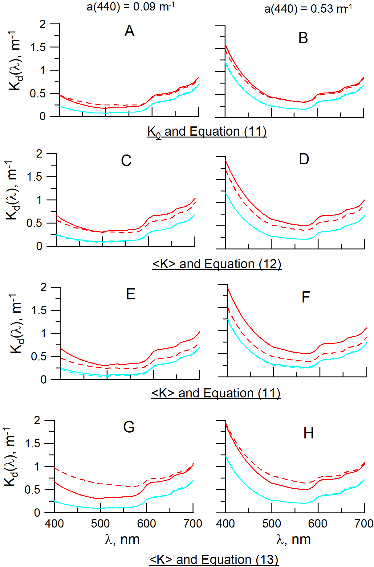
2.1. Field and Satellite Data for Modeling

In our work, we did not set out to reproduce the results of field measurements through numerical modeling; we used these results to approximate the input modeling parameters to the real conditions observed in the Barents Sea and Black Sea. The Shirshov Institute of Oceanology (SIORAS) conducts regular complex expeditions in these seas; one of the main tasks is to study coccolithophore blooms based on satellite and field measurements. In the Barents Sea, such expeditions have been conducted since 2014. During this period, five scientific cruises took place, in July–August 2014 and 2015, June–July 2016, and June–August 2017 and 2018 [5,6,29]. The complex optical measurements were carried out in almost all these expeditions (Figure 1 shows the main instruments) with simultaneous satellite ocean color observations (under favorable weather conditions), accompanied by hydrological and biogeochemical studies (the measurements were described the monograph [7] and articles [4,5]).
The results of the research in the Baltic, Norwegian, and Barents Seas in the 2014–2016 cruises demonstrate the effectiveness of an integrated approach to the use of optical methods combining the accuracy of contact ship measurements and the full coverage of the studied area with satellite images [29].
The 2017 voyage, the longest (51 days), proved to be the most fruitful; the measurements were carried out both at the drift stations and continuously on the ship’s course using a flow system [7]. At the drift stations, a submerged transparency meter measured the vertical profiles of seawater temperature and the beam attenuation coefficient; a laser spectrometer in the ship laboratory, measured the fluorescence spectra of colored dissolved organic matter (CDOM) and phytoplankton pigments in the water samples, taken from selected horizons; an Integrated Cavity Absorption Meter (ICAM) with an integrating sphere measured the absorption spectra of seawater, filtrates, and suspended particles [30,31]. A flow-through fluorometer with appropriate sensors, installed in a flow system, provided continuous measurements of the fluorescence of chlorophyll a (Chl a), CDOM, sea surface temperature (SST), and salinity (SSS). From the light measurements during daylight hours, we obtained data on the spectral upwelling radiance just beneath the sea surface Lu, spectral surface irradiance Es, the underwater Photosynthetically Available Radiation (PAR) values by a Li-COR device, and spectral values of the surface and underwater irradiance with E-meter and RAMSES devices (see Figure 1).
We took the data obtained at drift station 5580 north of the Kola peninsula (70.14° N, 35.27° E), the cruise AMK-68 2017 as the reference values for the Barents Sea input modeling parameters. As seen from the above text, we did not measure all parameters required for the numerical calculations. Still, we measured enough of them to derive the rest by using the appropriate models. We describe the algorithms used for that in Section 2.3. There we present the measured data which allowed the modeling mentioned above.
A spectral absorption meter ICAM provided the spectral absorption coefficients of the seawater (from the samples taken from different depths), a(λ); the filtrate (after filtration through a nuclear filter of 0.4μ), af(λ), and the particulate matter, ap(λ) (determined as the difference between the spectral values of the absorption coefficients of the seawater and the filtrate); ap(λ) = a(λ)−af(λ). The difference between the values of the filtrate and pure water absorption coefficients allowed for the estimation of the yellow substance (CDOM) absorption coefficient ag(λ) = af(λ)−aw(λ).
A submerged transparence meter PUM-A measured the vertical profiles of the beam attenuation coefficient c(530) at 530 nm with error 0.005 m−1 down to 200 m. After installing the plastic cuvette in the measuring channel, PUM-A can measure seawater samples in laboratory mode, in particular, in real-time, if it is involved in the flow system. Having the values of the attenuation and absorption coefficients, we obtained the scattering coefficient at 530 nm: b(530) = c(530)−a(530).
The measured data of the apparent optical characteristics, such as the spectral radiance reflectance ρ(λ), and the diffuse attenuation coefficient Kd(λ), allowed us to calculate the values of the inherent optical characteristics.
As seen from Figure 1, we had three devices to measure the downward and upward underwater irradiance that are useful for increasing the completeness of the information obtained and its accuracy. This is very important for the validation of the results of the numerical calculations.
A spectral underwater irradiation meter RAMSES ACC-VIS (TRIOS, Germany) has 190 spectral channels in the spectral range of 320–950 nm (spectral resolution is 3 nm) and an accuracy of ±5%. To conduct measurements in the sounding mode, we used a special frame and the data was transmitted to the ship laboratory by a cable. TRIOS provided calibration of the instrument to the National Institute of Standard and Technology (NIST) standards.
The other irradiance meter, E-meter (BIC 2100), has two measuring modules: the deck and underwater, which simultaneously measure the irradiance in four spectral bands 443, 490, 555, and 625 nm. The specialists from SIORAS modernized the device to perform measurements in an autonomous regime, without a cable. We calibrated the instrument at the SIORAS before each expedition, according to the working standard of the spectral irradiance density.
The PAR meter Li-192SA (Li-COR Company, USA–Canada) measured the surface and underwater quantum irradiance with an accuracy of ±5%. The underwater module included two submerged Li-192 photodiode sensors for measuring the downward and upward irradiance. The Li-190SA deck sensor measured the surface PAR. Our modernization made it possible to work autonomously without cables and with continuous recording of depth.
During our sea expeditions, we collected satellite data when the weather allowed us to get them. We used data from different satellite ocean color sensors, such as SeaWiFS, MODIS, OLCI, VIIRS, and AVHRR. Still, for constructing the long series data, the core information was from SeaWiFS and MODIS-Aqua, and we are now going to focus on the OLCI data [7].

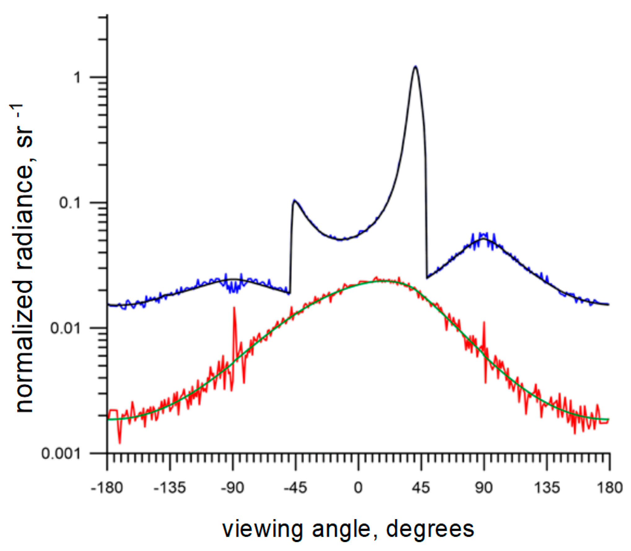
2.2. Calculation Method

We calculated the angular and spectral radiance distributions, the downward and upward irradiances, and others for real atmospheric and observation conditions, solving the radiative transfer equations by the matrix operator method developed in [32]. In our work, we use a modification [24] of this method.
We consider the ocean–atmosphere system as a set of plane-parallel homogeneous layers. To solve RTE (without taking into account the effects of polarization), we should specify the absorption coefficient of sea water a(λ) and the volume scattering function (VSF) β(θ,λ), where θ is the scattering angle and λ is the wavelength.
For the atmosphere, we use a two-layer model: the upper layer with Rayleigh optical thickness [33] and Rayleigh phase function, and the lower layer with the model phase scattering function by Gordon and Castaño [34] and the optical thickness τ = τ a ( 869 ) ( 869 λ ) A , where Angstrom index A and the aerosol optical thickness τa(869) are taken from the data of satellite color scanners.
The surface is considered as a separate layer. Formulas for a smooth surface are presented below; for a wind-roughened surface, we used the results of [35,36].
The layers are numbered downward from 1 to N; their optical properties are completely determined by optical thickness Δτi = cΔzi, single scattering albedo ω, and the phase function pi(θ). The radiances and irradiances can be calculated at the levels numbered as 0, 1, … N, the i-th level being a boundary between the layers i and i+1. Hence, level 0 corresponds to the top of the atmosphere (TOA), and level N is the bottom. The version of the matrix operator method used here is based on recurrence formulas (see below) applied to single-layer reflection and transmission operators. A distinctive feature of the algorithm is the ability to use the results obtained by different numerical methods in one calculation. The result for a multilayer system that includes (or does not include) a surface can be assembled from pre-calculated elements.
For each layer we define two reflectances, r i ( Ω , Ω 0 ) and r i ˜ ( Ω , Ω 0 ) , and two transmittances t i ( Ω , Ω 0 ) and t i ˜ ( Ω , Ω 0 ) . By definition, r i ( Ω , Ω 0 ) is the intensity of upwelling radiation in the direction Ω = ( μ φ ) if the incident downwelling radiance is L ( Ω ) = δ ( Ω , Ω 0 ) (µ = cos θ; θ and ϕ are the zenith and azimuthal angles of the incident light, µ is always positive here). The definition of transmittance is obvious; a tilde corresponds to the case of upwelling incident radiation in the water and atmosphere layers r i ( Ω , Ω i ) = r i ˜ ( Ω , Ω i ) and t i ( Ω , Ω i ) = t ˜ ( Ω , Ω i ) This does not apply to the surface; for example, for a smooth surface we have the formulas
r i ( Ω , Ω 0 ) = r f r ( μ , n w ) δ ( μ μ 0 ) δ ( φ φ 0 ) ,   r i ˜ ( Ω , Ω 0 ) = r f r ( μ , 1 n w ) δ ( μ μ 0 ) t i ( Ω , Ω 0 ) = t f r ( μ , n w ) n w 2 δ ( 1 n w 2 ( 1 μ 2 μ 0 ) δ ( φ φ 0 ) t i ˜ ( Ω , Ω 0 ) = t f r ( μ , n w ) n w 2 δ ( 1 n w 2 ( 1 μ 2 μ 0 ) δ ( φ φ 0 )
where rfr(μ,nw) is the Fresnel reflection coefficient, nw is the water refractive index, and tfr(μ,nw) = 1− rfr(nw).
From elementary probabilistic considerations, it follows that the formulas for the upwelling radiances Un and the downwelling radiances Dn at level n can be expressed in terms of the transmittance Tn and the reflectance Rn for truncated systems. In operator form,
D n = ( 1 ^ R ˜ n R n ) 1 T n ,     U n = R n D n
where Tn is the transmittance of the system including layers 1,2, … n, R ˜ n is backward reflectance for the same system, Rn—reflectance for layers n+1, n+2, … N, RN is the bidirectional reflectance distribution function of the bottom, and 1 ^ is the unity operator δ(μ−μ0 )δ(φ−φ0 ).
To calculate the truncated operators, we use the following recurrence formulas:
R n = r n + 1 + t ˜ n + 1 R n + 1 ( 1 ^ r ˜ n + 1 R n + 1 ) 1 t n + 1
Note that the transmittance operator Tn is not involved in calculation of the top of the atmosphere (TOA) radiance Lt ≡ R0.
T n = t n ( 1 ^ R ˜ n 1 r n ) 1 T n 1
R ˜ n = r ˜ n + t n R ˜ n 1 ( 1 ^ r n 1 R ˜ n 1 ) 1 t ˜ n
Equations (2)–(5) are a complete system of recurrence formulas for calculating the required radiances. The initial condition to Equation (2) is the bottom bi-directional reflectivity RN, the initial conditions of the coupled system of Equations (3) and (4) are T0 = 1 ^ and R ˜ 0 = 0 . The radiance at the TOA can be calculated in a single pass of N steps, starting from the bottom and ending with the TOA. To find the radiances at other levels, a second pass from the top layer down is required.
To obtain a working algorithm, the direct radiance should be separated from the diffuse one. Let us denote
r n = r n d i r + r n ,   t n = t n d i r + t n ,   R n = R n d i r + R n ,   T n = T n d i r + T n
where the operators denoted by the superscript dir are singular, i.e., proportional to a delta function, and boldface characters denote regular (not containing any delta functions) parts of the operators. Substituting this into Equations (3)–(5), one can obtain a system of Fredholm integral equations of the second kind with a kernel yielding a compact operator. Such equations can be easily solved using a standard numerical technique. Assuming that all of the above operators are axially symmetric, we can expand them into a Fourier series in the parameter φ-φ0, and obtain a decoupled system of recurrence formulas of the same form, with integration not over Ω but over the one-dimensional parameter μ. To find the solution, it is sufficient to choose a discretization method, i.e., a set of nodes and weights in a quadrature formula. Then the problem reduces to solving a system of linear algebraic equations. For atmospheric layers, we use the Gauss quadrature; for water layers, a set of nodes and weights proposed in [23]; For the surface, a combination of both.
To calculate the one-layer reflectance and transmittance, two methods were used: the discrete ordinate method [37] or Monte Carlo method. The discrete ordinate method and the program DISORT are described in detail in a series of publications by K. Stamnes et al. [38,39]. We use the part of the code intended for the one-layer system [38], simplified and modified so that it calculates and stores full matrices, rather than radiances for a limited set of user-defined angles. The result of the calculation can be stored on a hard disk and used afterwards as an imported one-layer operator. The Monte Carlo method has been included mainly for checking purpose (see Section 5.1).

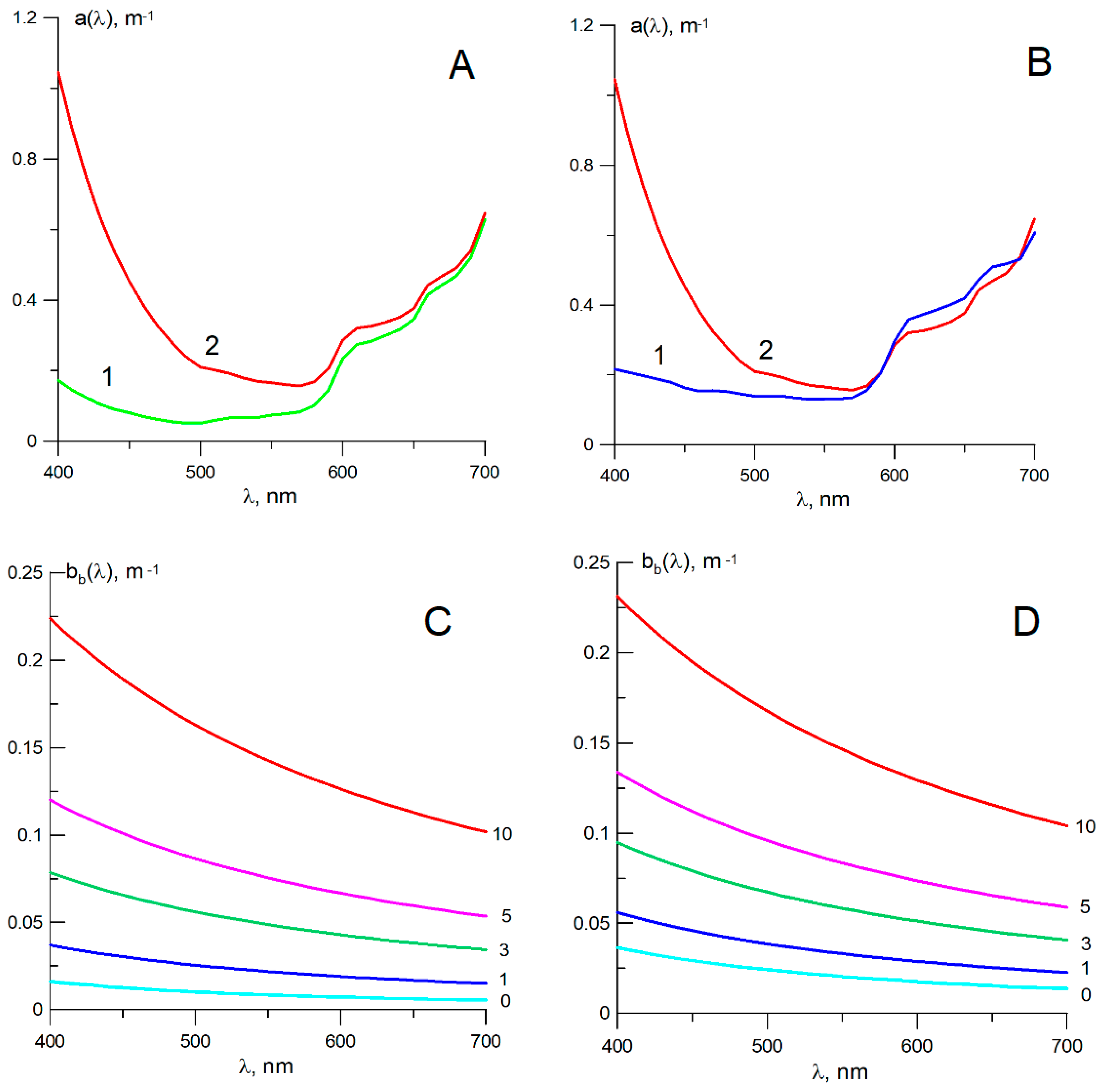
2.3. Input Parameters for the Modeling

As pointed out in Section 2.2, for the numerical calculation of the underwater radiance, we need a knowledge of the seawater absorption coefficient a(λ) and the seawater volume scattering function (VSF) β(θ,λ) (where θ is the scattering angle and λ is the wavelength). At that, we have to know the above parameters not only for the seawater as a whole, but for each of its optically active components. To bring our model to reality, as close as possible, we consider not only the plated cells and coccoliths, but the non-coccolithophore components, such as particles of another origin, colored organic matter, and of course the water itself. We used the parameters, based on the real optical and biological data, measured in our sea expeditions. Table 1 shows the origin of the user settings. Below we present the results obtained at drift stations in the Black Sea and Barents Sea, a procedure for the calculation of the coccolithophore optical characteristics is described afterwards.
For the Black Sea, we used the data from two stations, both in the northeastern part of the Black Sea near Gelendzhik, ~45°N, 38°E, at a depth of 30 m [31]. See Station 1_08.06.2017 as an example of a very intensive coccolithophore bloom with a concentration of coccolithophores at Ncoc = 8.2 × 10⁶ cell/L, and Station 1_08.06.2018 with no CB for assessing the effect of the “non-coccolithophore” particles (see below). At Station 1_08.06.2017, the favorable weather conditions (the solar zenith θ0 was 25°, a calm sea) supported both our field measurements and the satellite observations. From MODIS satellite data, the aerosol optical thickness τa(869) equaled 0.146 and the Angstrom parameter 1.70.
We assumed the total absorption coefficient was a sum of the contributions from pure water and the yellow substance (CDOM), neglecting the phytoplankton absorption, because, according to the ICAM data (see Section 2.1), it made an insignificant contribution. As the absorption coefficient for pure water, we took the data by [45] and the spectral CDOM absorption slope Syel = 0.017 nm−1 for the range 400–500 nm and 0.011 nm−1 for 500–700 nm [43].
As the absorption input parameter, we used the value of the seawater absorption coefficient a(440) = 0.09 m−1 at 440 nm, according to the ICAM data [31]. For studying the absorption effect on the light field and its integral parameters, we performed our modeling not only with the above input parameter but also with much higher inputs, up to 0.53 m−1.
As the input parameter of the coccolithophore bloom, we used the plated cell concentration Ncoc, and varied it from 0 to 107 cell/L. For the ratio of the coccolith concentration Nlith to the plated cell concentration Ncoc (Nlith/Ncoc), we assumed it to be equal to 35, according to measurements at the station 1_08.06.2017.
We also took into account the existence of the “non-coccolithophore” particles supplied by river runoff [4]; their optical parameters were calculated by using a model [40,41,42,43]. This model was built on the basis of the directly measured VSF data and validated by the results of the analysis of marine particles by microscopic and chemical studies and the retrieval of the size distribution of marine particles from the VSF. Using the model, we estimated the volume concentrations of small (radiuses less than 1 μ) and large (≥1 μ) “non-coccolithophore” particles from the measured data of 2018 under a no coccolithophore bloom condition [31], and obtained vs = 0.14 cm3 m−3 for the fine fraction and vl = 0.78 cm3 m−3 for the coarse fraction. The concentration of “non-coccolithophore” particles was assumed to be independent from the coccolithophore concentration and constant.
For the Barents Sea, we derived the model parameters based on the data of 15.07.2017 at station 5580 of the 68th cruise of R/V “Akademik Mstislav Keldysh”. The measured concentration of the coccolithophore plated cells was approximately Ncoc = 5 × 10⁶ cell/L, the detached coccoliths Nlith = 1.5 × 10⁸ cell/L.
After calculating the bcoc, blith, bbcoc, and bblith, we obtained the bn and bbn values of the non-coccolithophore particles: bn = b – (bcoc + blith), bbn = bb – (bbcoc + bblith), where the b and bb values are from the measured data (see Table 1). The obtained bn and bbn values allowed us to find the parameters vs and vl of the two-parameter model of the scattering properties [42,46]. Performing the calculation, we got vs = 0.35 cm3 m−3 and vl = 4.62 cm3 m−3.
As to the calculation of the coccolithophore optical characteristics, we can mention several publications which considered the results of theoretical calculations and experimental studies of the optical characteristics of coccoliths and plated cells [47,48,49,50,51,52]; we discuss them in Section 5.2.
To create a set of the input parameters for a calculation of the coccolithophore optical characteristics, we used the data of the work [51] which presents an almost full set of the optical characteristics, except polarization properties, obtained from comprehensive laboratory measurements. These measurements provided spectral data on the beam attenuation cross sections (m2 particle−l) for coccoliths, plated cells, and naked cells, and the values of the volume scattering function (VSF) at six wavelengths. They measured VSF at every degree between 10° and 170° and, for calculating the bb values, extrapolated the measured data from 170° to 180° by assuming VSF(θ) for 170–180° was constant. They estimated the error in the calculation of bb as ± 1%.
For our modeling, we need the whole phase scattering function (PSF) from 0° to 180° and to get it, we analyzed the data of [49] which comprise the Mueller scattering matrix, backscattering probability, and depolarization ratio for Emiliania huxleyi. For their numerical calculations, the authors used a realistic non-spherical model, based on electron micrographs of coccolithophore cells, and the discrete dipole approximation. They presented the phase scattering functions for different cell sizes with the equivalent diameters of the cell from 3.75 to 6.75 μ for the plated cells and from 1.63 to 4.73 μ for coccoliths. We compared their calculated functions and different combinations of them with the VSF from [51], sorting out the appropriate particle concentration. Figure 2 shows the final result as compared with the phase scattering functions for the Black Sea and Barents Sea non-coccolithophore particulates.
As seen from Figure 2A, the phase scattering functions for the plated cells and coccoliths are close to each other, as noted in [51], and they are not as elongated as the functions for non-coccolithophore particulates in Figure 2B. The comparison between the integral parameters for the coccolithophore systems (including both the plated cells and coccoliths) and for the non-coccolithophore particles in the Black Sea confirms the observed difference: the backscattering probability b ˜ b = bb/b at 555 nm equals 0.027 for the former and 0.017 for the latter; the values of the average cosine of the single scattering are equal to 0.892 and 0.922, respectively. The most elongated PSF for the in non-coccolithophore particles in the Barents Sea was b ˜ b ( 555 ) = 0.0091 , < cos θ 0.949 .
Figure 3 presents the spectral values of the absorption and the particle backscattering coefficients for the Black Sea and Barents Sea used in our numerical simulations.
There is a significant difference between the Black Sea and Barents Sea in their values of the absorption coefficient at a wavelength less than 550 nm—the values at 440 nm equal 0.09 and 018 m−1, respectively (see Table 2 below). A similar difference is also seen in Figure 3C,D between the values of the backscattering coefficient for Ncoc = 0: 0.008 and 0.020 m−1, respectively (Table 2).
The set of the optical characteristics in Table 2 looks nice for the modeling purposes because it presents a wide variety of the ratio between two the main processes determining the light propagation in the water medium: the scattering and absorption; the ratio b/a at 440 nm changes by a factor of about 70 at 555 nm—more than a factor of 22.

3. Results Obtained

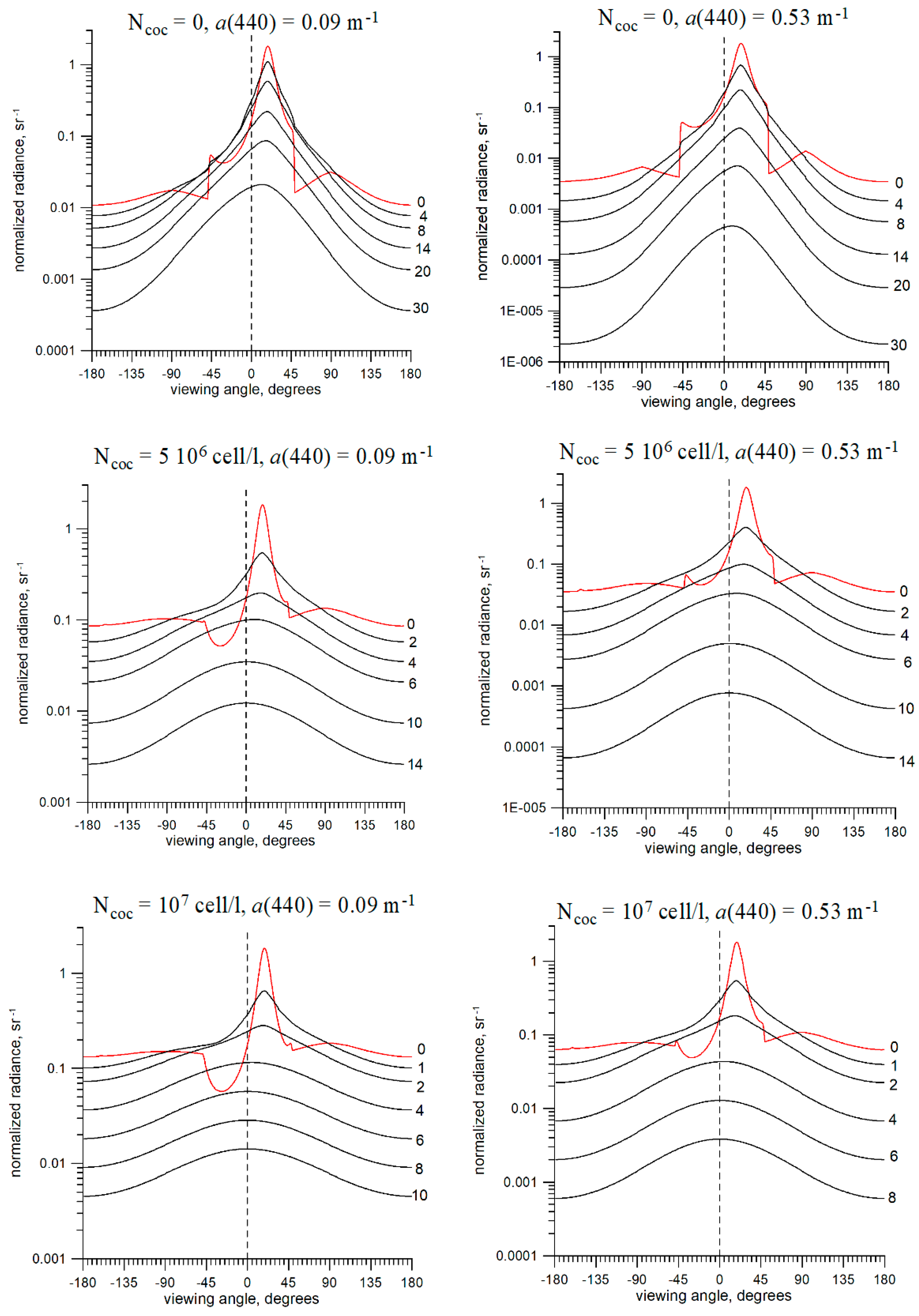
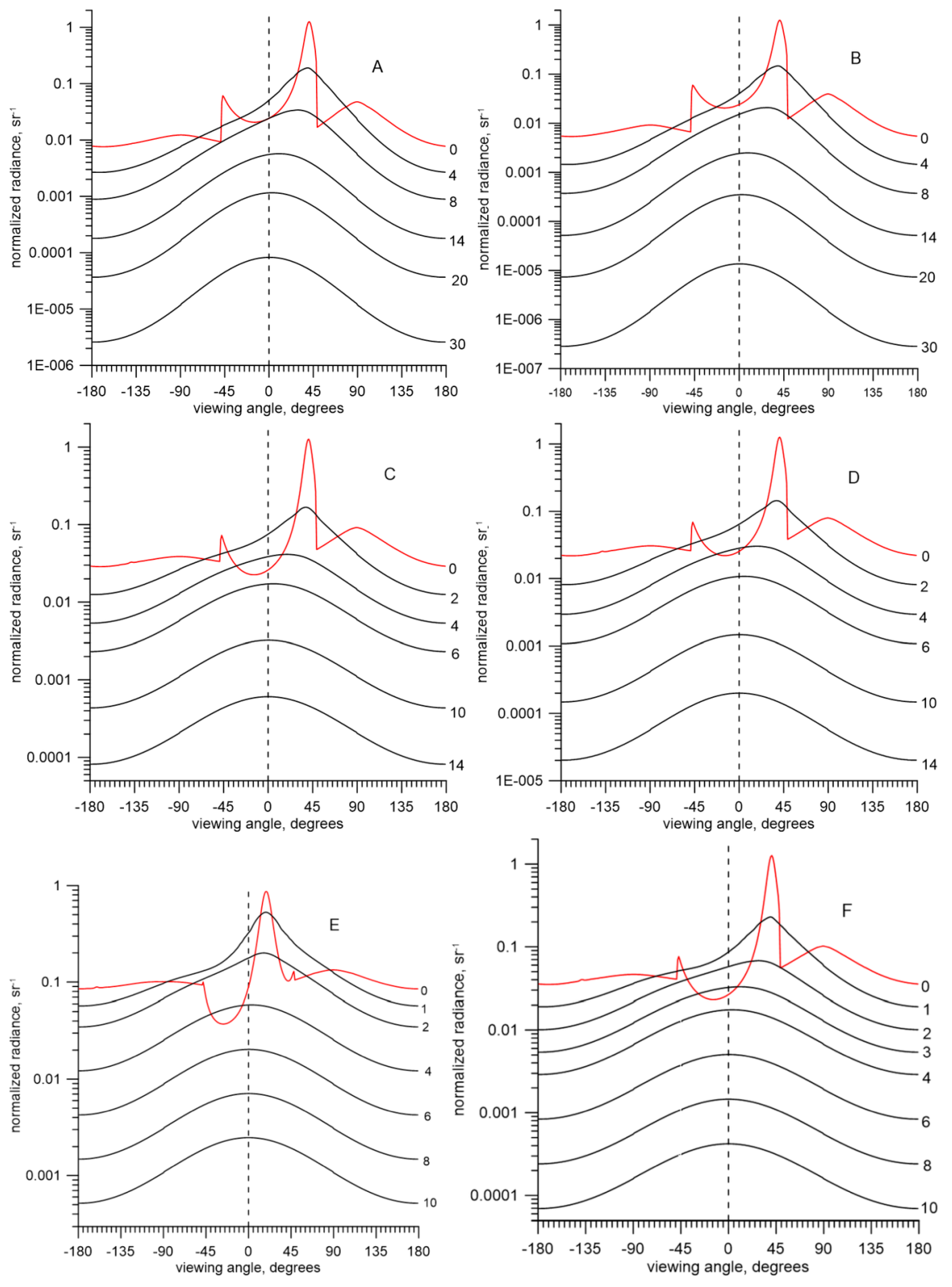
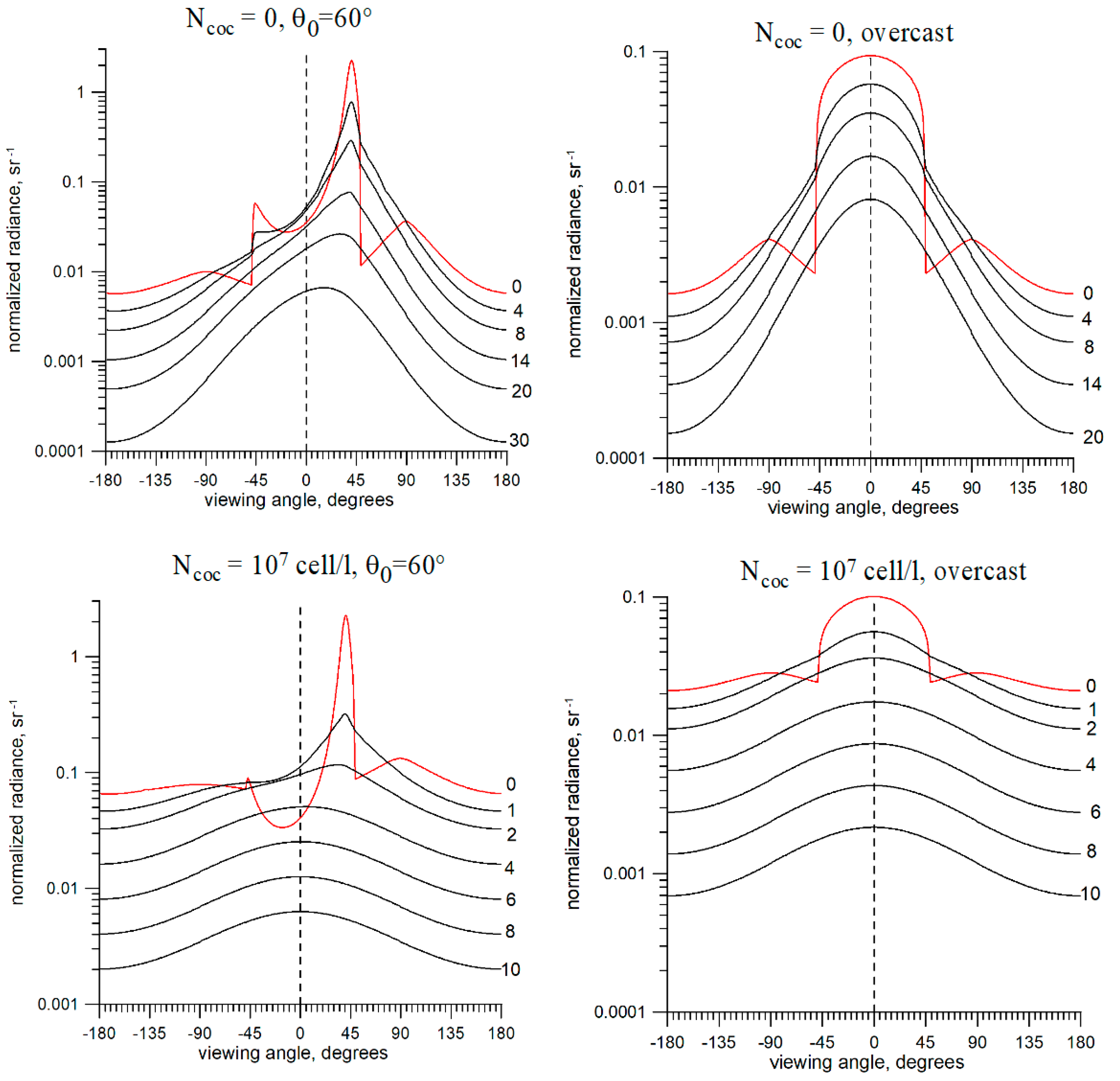
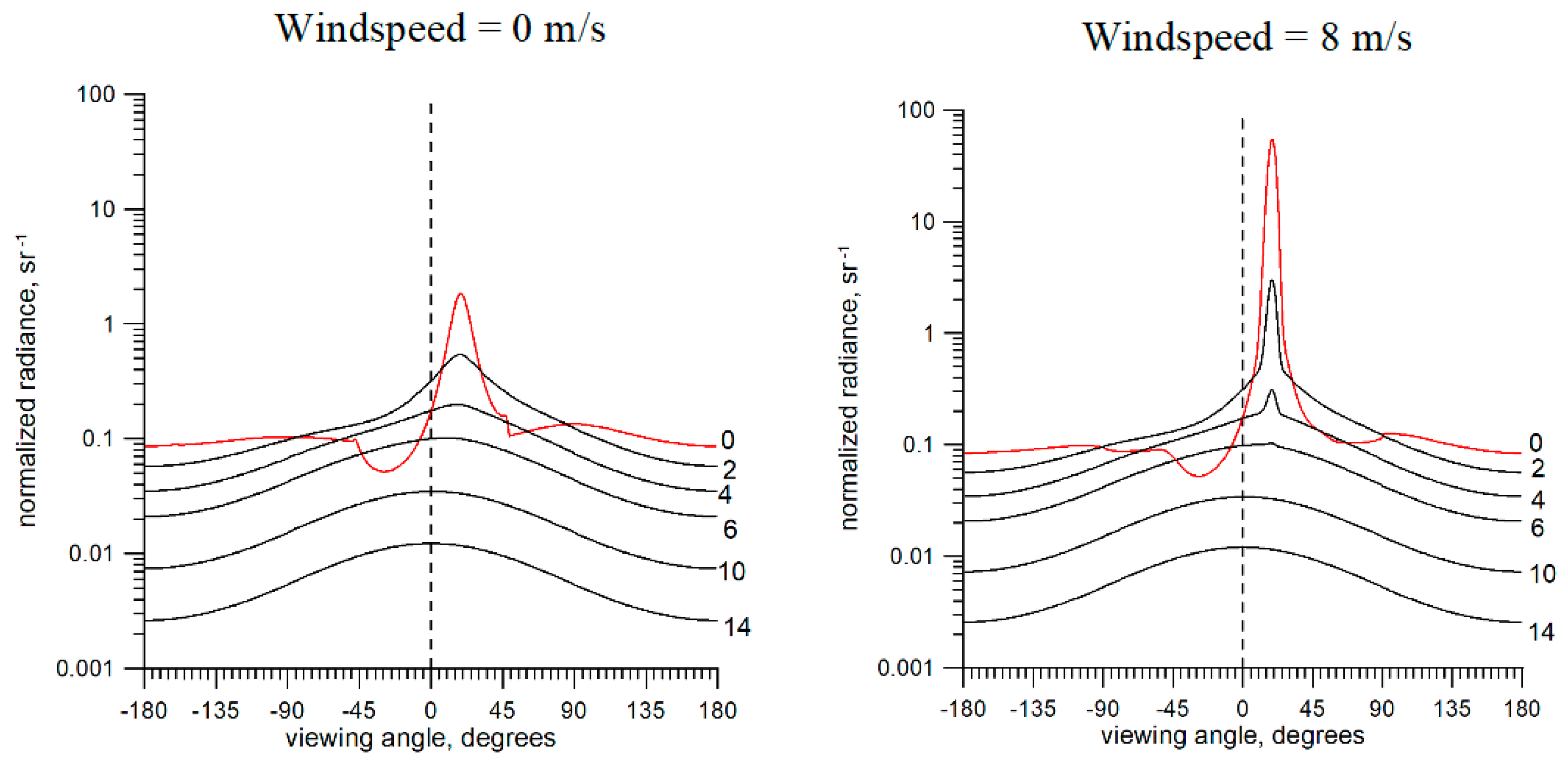
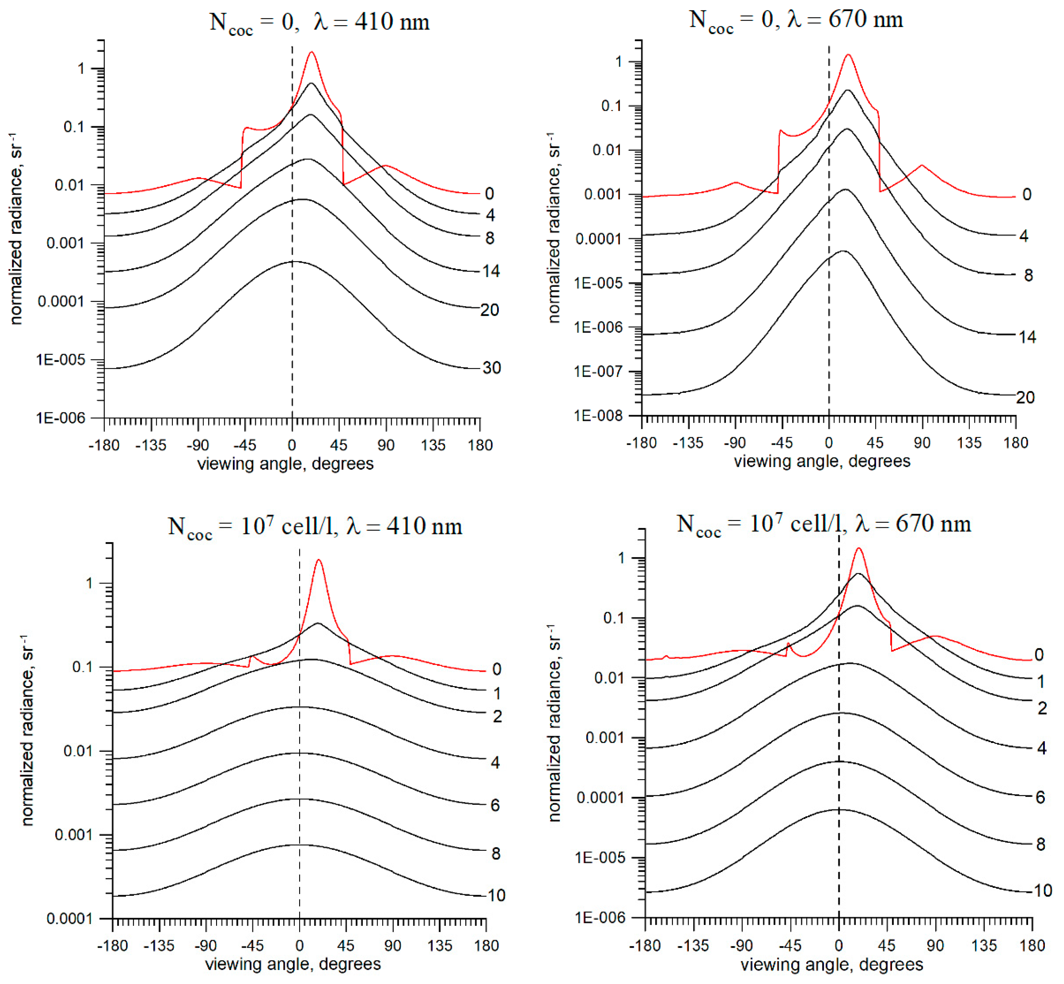
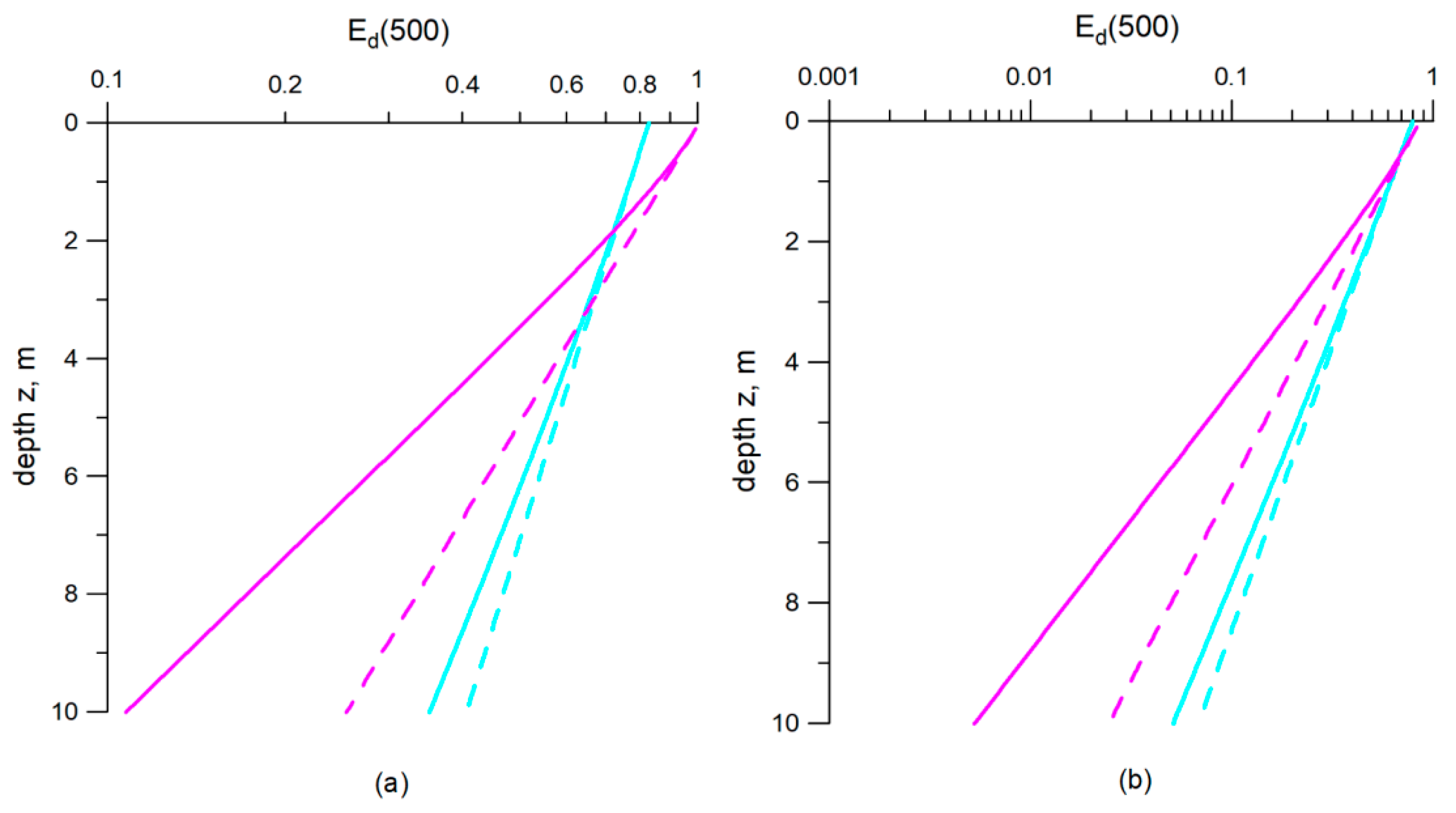
3.1. Effect of the Coccolithophore Bloom on the Underwater Light Field

The features of the underwater light fields depend on the seawater optical characteristics and their vertical distribution and the illumination conditions (solar zenith and azimuthal angles, atmosphere condition, cloudiness, sea surface state). We considered the general topics of the problem, including the approaches, in previous sections, now we present the results of our numerical calculations for different conditions and discuss them.
Figure 4, Figure 5, Figure 6, Figure 7 and Figure 8 show, for the Black Sea and the Barents Sea, the angular distributions of the underwater radiance at the plane of the sun, depending on the coccolithophore concentration Ncoc and the absorption coefficient a(440) for different observation conditions, such as the solar zenith angle θ0, the cloudiness, and the wind speed.
As already noted in the introduction, the research of laws and features of underwater light fields has been going on for several decades, including field and laboratory studies (with artificial media, imitating real seawater optical properties) and modeling. The last has several important advantages (see Introduction).
To date, there are general ideas developed about solar radiation propagation in the water column. One of these is the occurrence of the asymptotic radiance distribution in deep waters. Figure 4, Figure 5, Figure 6, Figure 7 and Figure 8 display this feature, and later we will pay special attention to it. We start with the subsurface horizon, just beneath the sea surface (commonly referred 0, as opposed to 0+, just above the sea surface). The red curves in Figure 4, Figure 5, Figure 6, Figure 7 and Figure 8 present the distributions at horizon 0. We see a classic picture showing the so-called Snellius circle, which corresponds to radiation entering the water column through the sea surface. This radiation propagates inside a cone with a cone angle of approximately 48°, corresponding to the maximum refraction angle in the absence of surface waves (wind speed is 0). We see the Snellius circle better in the bloom absence (Ncoc = 0); a strong scattering washes it out even directly below the surface.
Figure 4, Figure 5, Figure 6, Figure 7 and Figure 8 demonstrate the transformation of the angular radiance distributions with increasing depth. At small depths, we observe the asymmetry of distributions associated with direct sunlight—the maximum of the angular distribution corresponds to the solar zenith angle after refraction when crossing the sea surface. At large depths, the angular distribution gradually becomes symmetrical about the vertical axis and unchangeable with further increasing depth. Such a distribution depends only on the seawater optical characteristics at these depths and not at all on the illumination conditions. This is a so-called asymptotic regime and we discuss it more detail in Section 5.3.
Comparing Figure 4 and Figure 5, one can see the similarity of the presented results, despite the notable difference in the optical characteristics of the considered seas and the solar zenith angles.
Figure 5 shows the analogical angular distributions of the underwater radiance for the Barents Sea. The difference between distributions is more pronounced in the absence of blooming (Ncoc = 0), it is displayed in the shape of the distributions and the absolute radiance values. The comparison of distributions in Figure 4 (left) and Figure 6 (left) between the sun angles of 25° and 60° for the Black Sea shows a significant difference only for subsurface horizons and in the absence of blooming. Figure 6 (on the right) shows that cloud conditions significantly affect both the shape of the angular distribution and the absolute radiance values. The changes in the sea surface state due to an increase in wind speed has a significant effect on the crossing of the sea surface by direct sunlight and near the maximum (Figure 7, θ = 25°).
Analyzing the angular radiance distributions and absolute values of the underwater radiance in Figure 4 and Figure 5 and Table 3, we can note the effect both of the scattering and absorption. The absorption causes a vertical elongation of the angular distributions, increasing it (we characterize this parameter as the ratio of the normalized radiances for 0° and 90°). This effect is more significant for the Black Sea, where the initial absorption is less (for the Black Sea, Ncoc = 5 × 10⁶ cell/L, this ratio increased by the factor 1.5, for the Barents Sea, only 1.2). It is the same for the asymptotic diffuse attenuation coefficient k: it increased for a(440) = 0.53 m−1 by a factor of 1.7 for the Black Sea (Ncoc = 5 × 10⁶ cell/L), and only 1.2 for the Barents Sea (see Table 3).
The results of our calculations allow us to get information about the effect of coccolithophore blooms on the satellite ocean color observations. Figure 4, Figure 5, Figure 6, Figure 7 and Figure 8 comprise the data on the upwelling angular radiance distributions within the angle ranges of −180° ÷ (−90°) and 90° ÷ 180. The red curves in these figures provide us with the useful information about the impact of different factors on the upwelling radiance: the coccolithophore bloom intensity, the CDOM absorption (Figure 4 and Figure 5), the effects of the solar zenith angle and cloudiness (Figure 6), and the sea surface state determined by wind speed (Figure 7).
Figure 8 shows the influence of the coccolithophore bloom intensity and the CDOM absorption on the angular and spectral dependencies of the subsurface radiance reflectance rrs. The observation at nadir corresponds to the viewing angle of ±180°, and we can note that a CB with Ncoc = 107 cell/L results in increasing rrs by about an order of magnitude at 410 nm, and by about a factor of 20 at 670 nm as compared with no bloom. We can also observe a weak angular dependency of rrs at 410 nm for the case of Ncoc = 107 cell/L. In both cases, Ncoc = 0 or 107 cell/L, the rrs value is much higher at 410 nm than at 670 nm; the reason for that is that there is a significant difference between the values of the absorption coefficient a(410) and a(670), as well seen in Figure 3. However, we can note that the ratio rrs(410)/rrs(670) is less under a CB than in its absence. We can explain that by the effect of spectral dependency of bb(λ) on the parameter u = bb/( a+ bb); as seen from Figure 3, the bb coefficient is noticeably higher at 410 nm than at 670 nm for Ncoc = 107 cell/L. We can explain the observed changes by the behavior of the ratio of the backscattering and absorption coefficients bb/a that is seen in Figure 3.

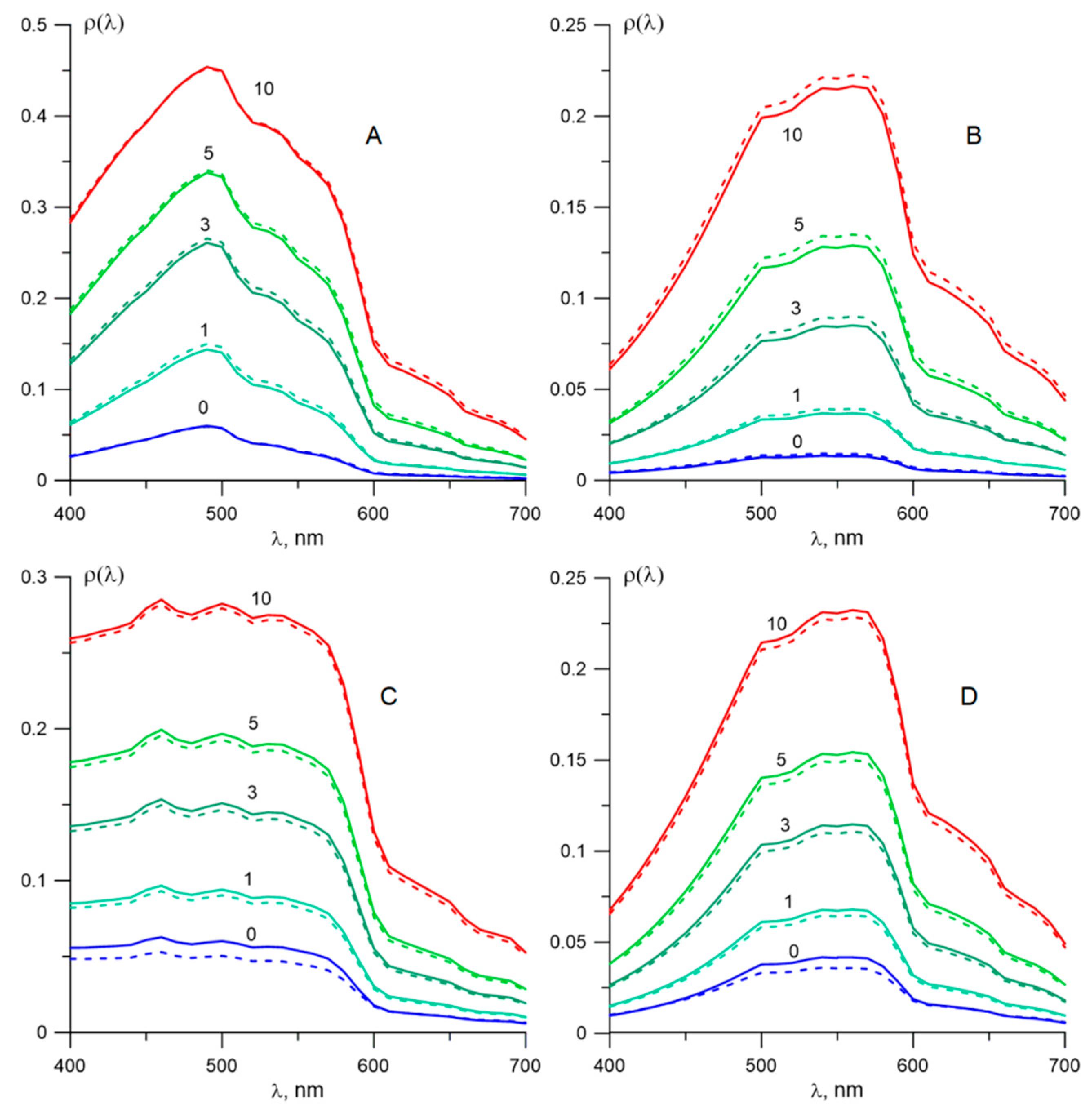
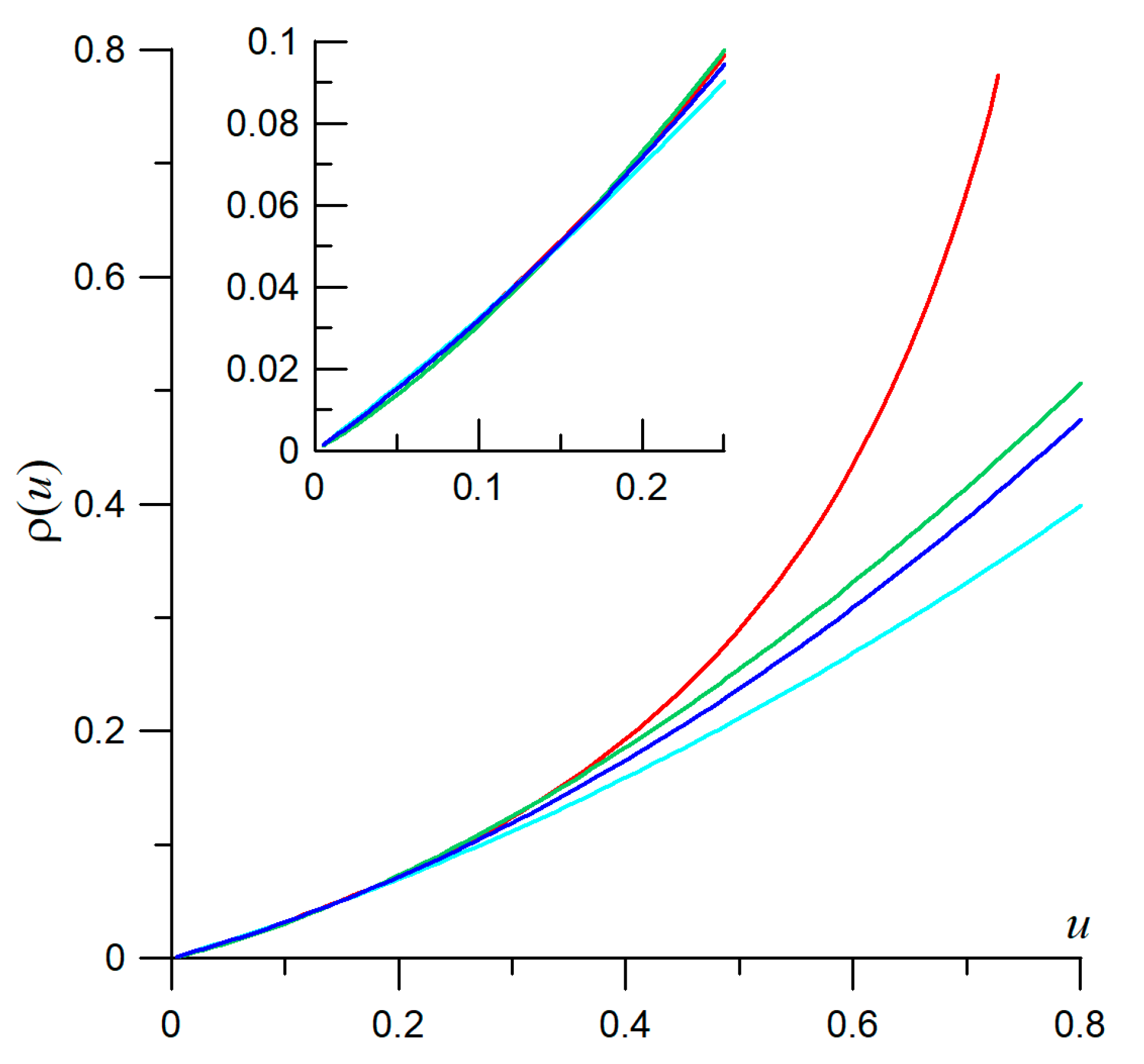
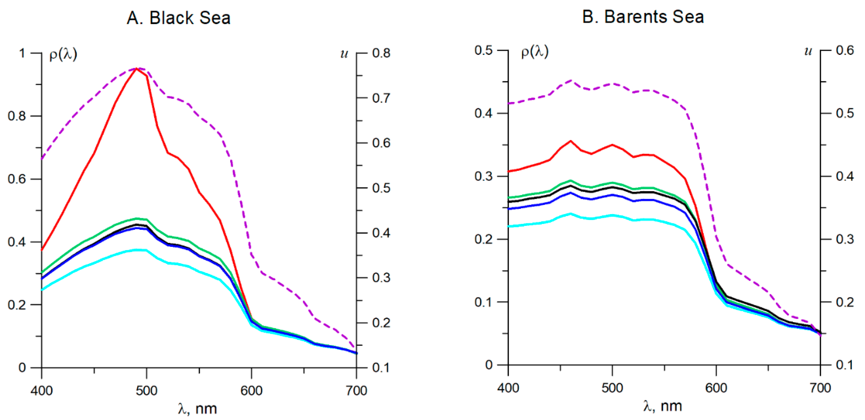
3.2. Coccolithophore Bloom Impact on the Water Radiance Reflectance

In Section 3.1, we focused on the angular distributions of the underwater radiance including the distribution just beneath the sea surface that determines the so-called water-leaving radiance just above the sea surface. The main effect of the coccolithophore bloom on the upwelling radiance is the sharp increase in its absolute values, but the processing algorithms for satellite ocean color data are based on the analysis of the spectral values measured by satellite sensors. Keeping this in mind, we consider in this section the spectral values of the water radiance reflectance ρ(λ).
Figure 9 shows the spectral values of ρ(λ) obtained by numerical calculation (see Section 2). We consider the changes of ρ(λ) depending on the coccolithophore concentration Ncoc for the Black Sea (the upper row in Figure 9) and the Barents Sea (the lower row). For each sea, we consider two cases of the spectral absorption (see Figure 3A,B): a(440) = 0.09 m−1 and 0.53 m−1 for the Black Sea, and 0.18 m−1 and 0.53 m−1 for the Barents Sea (the low values relate to Figure 9A,C and the high, Figure 9B,D).
For each value of the coccolithophore concentration we consider two variants of the observation conditions: clear sky with the solar zenith angles θ0 = 25° and 60° for the Black Sea, and clear sky with the solar zenith angle 60° and overcast for the Barents Sea (dashed lines show the second variants). As seen for the Black Sea, an increase in the solar zenith angle leads to a slight change in ρ(λ). For the Barents Sea, water radiance reflectance for θ0 = 60° is greater than for overcast. The difference is at a maximum for Ncoc = 0 and a(440) = 0.18 m−1, but even here it does not exceed 6%.
Comparing Figure 9A,C, it can be noted that all the curves in the blue part of the spectrum are much flatter for the Barents Sea than for the Black Sea. This can be easily explained: the spectral dependence of ρ is largely determined by the parameter u = bb/(a + bb), and therefore by the coefficient a. Spectral dependences of ρ shown in the right panel of the figure are much more similar due to coincidence of absorption coefficients. For Ncoc = 107 cell/L, and to a large extent Ncoc = 5 × 10⁶ cell/L, these curves are difficult to distinguish, since the scattering here is mainly determined by coccolithophores. At lower values of Ncoc, this similarity persists, although the scattering here is mainly due to non-coccolithophore suspension. The fact is that in this range of Ncoc values, the shapes of the ρ(λ) curves are largely determined by the spectral dependence of the absorption coefficient.
To track changes in the shape of the spectra ρ(λ) depending on the Ncoc concentration, we took the ratio ρ(490)/ρ(550) of the ρ spectral values at 490 and 550 nm; that is close to the parameters which are used in the processing algorithms OC2M and KD2M for the MODIS data [53]. Table 4 presents the results obtained.
The data in Table 4 correspond to the changes in the spectra ρ(λ) in Figure 9. In the case of significant absorption (a(440) = 0.53 m−1 and 0.18 m−1), the ratio ρ(490)/ρ(550) in Table 4 depends weakly on Ncoc concentration and varies no more than 6%. For weak absorption (a(440) = 0.09 m−1), we observe a significant decrease in the ratio ρ(490)/ρ(550) with increasing Ncoc. Even for Ncoc = 106 cell/L, the value of ρ(490)/ρ(550) reduces by 10%, as compared with the bloom absence (Ncoc = 0); for an intense bloom (Ncoc ≥ 5 × 10⁶ cell/L), the ratio ρ(490)/ρ(550) decreases by more than 26%. These results indicate the possibility of using the above parameter in the weak absorption case, and the need to choose another one for significant absorption.

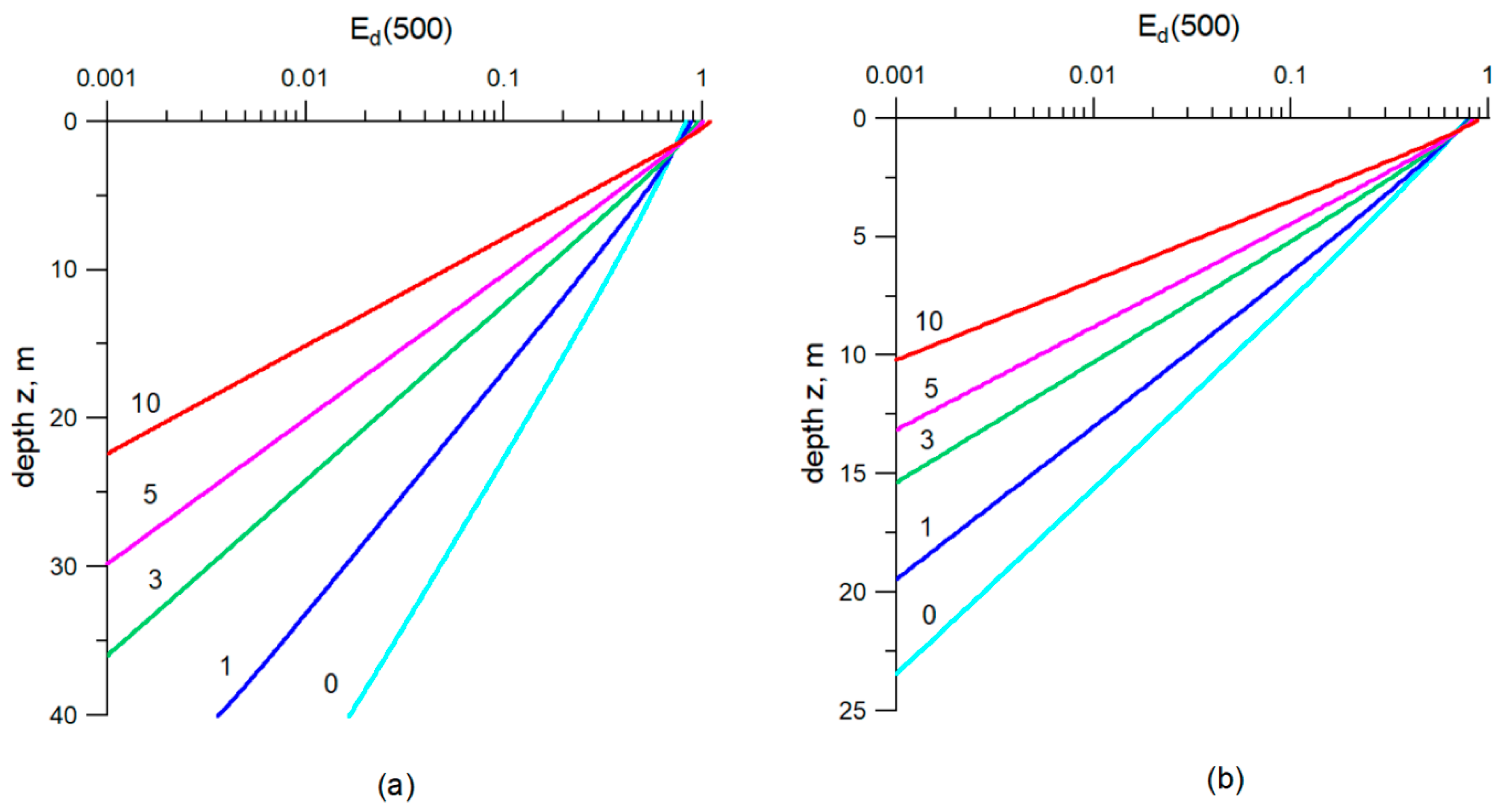
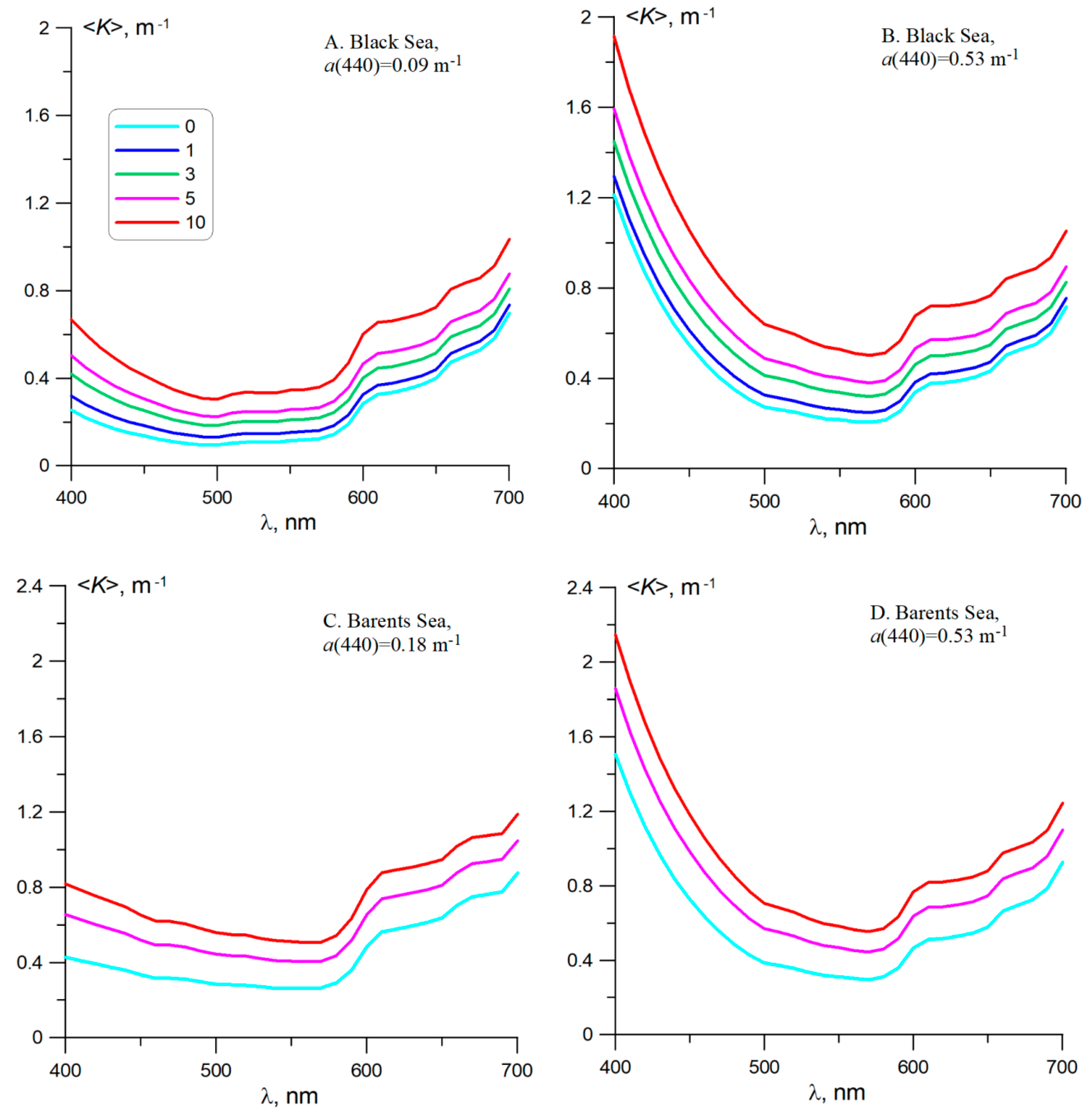
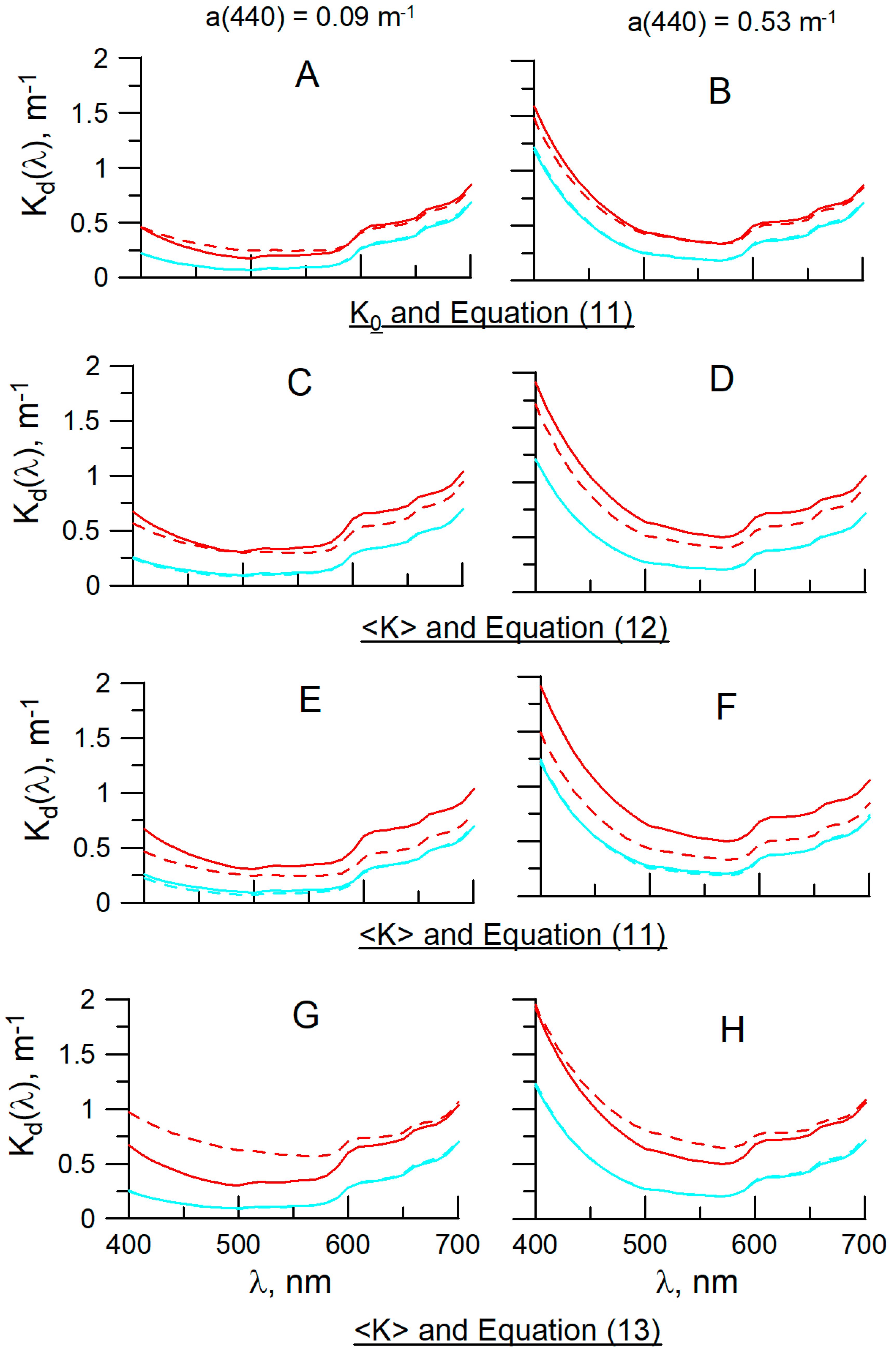
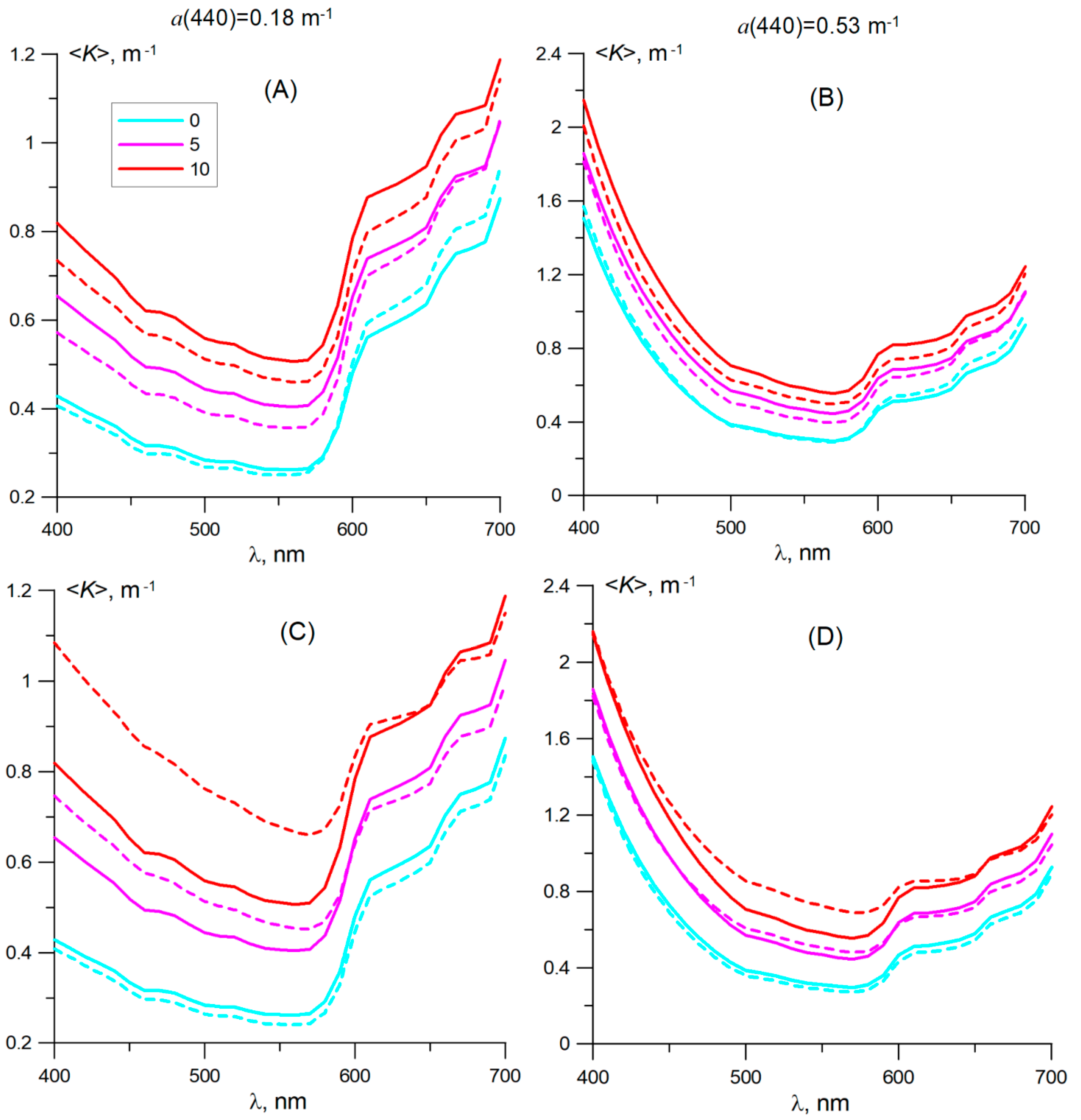
3.3. Coccolithophore Impact on the Diffuse Attenuation Coefficient

In this section, we consider the propagation of the solar radiation in the water column, focusing on the effect of the coccolithophore bloom on this process. Usually, we assume for the attenuation of the underwater irradiance with depth an exponential law with an exponent Kd called the diffuse attenuation coefficient. Kd depends strongly on the wavelength and the angular structure of the propagating light stream; this problem was discussed in detail in [54]; We consider the applicability of the approximate formulas in Section 4.2.
Figure 10 shows the vertical profiles of the downward irradiance Ed(500) calculated for the case of the Black Sea, depending on the coccolithophore concentration Ncoc and the absorption coefficient a(440). As seen, both factors have a significant effect on the depth of the photic layer Z1% (where PAR decreases to 1% of its surface value). In the case of a(440) = 0.09 m−1 and the CB absence, the Z1% value is more than 40 m, it decreases to 34.5 m for Ncoc = 1 × 10⁶ cell/L, and Z1% is only 15.5 m for Ncoc = 107 cell/L.
Table 5 presents the depth of the photic layer Z1% for the cases of the Black and Barents Seas, depending on the coccolithophore concentration Ncoc, the absorption coefficient a(440), and illumination conditions. If the CB is absent, the depth of the photic layer Z1% is much less in the Barents Sea than in the Black Sea, which is explained by a large amount of “non-coccolithophore” particles. In both seas, the intense CB leads to a significant reduction in the Z1% value. For Ncoc = 107 cell/L, it decreases by a factor of two, regardless of the value of a(440). The Z1% depends on the illumination conditions, in particular, on the low sun. The Z1% is less than in overcast conditions, and in this case, it is less than with the high sun; the influence of illumination conditions mitigates with increasing Ncoc.
It is known that the diffuse attenuation coefficient Kd depends on the depth, even if the optical properties do not change with depth, but how can the CB affect these changes? It seems that the profiles of the downward irradiation on a semi-logarithmic scale (Figure 10) are straight lines and there is no difference in the slope depending on the depth, but this is not so.
Figure 11 shows the difference between the profiles of the downward irradiation obtained as a result of numerical simulation, with the assumption that Kd is constant and equal to K0. In this case, we calculated the value K0 in the uppermost layer 0–0.1 m (as the increments of depth for calculations are 0.1 m) and then the irradiance profile using the exponential law with Kd = K0 = const. It is seen that even in the absence of a CB, the use of K0 overestimates the values of irradiance obtained; the difference for Ed estimates with a depth is especially large for small absorption and high coccolithophore concentrations.
Obviously, the use of K0 for calculating the attenuation of light with depth in the CB case results in large errors; it is better to use the Kd average for the photic layer. For example, in [54], the diffuse attenuation coefficient <K> was introduced as the average for layer τ10, in which the irradiance decreases by a factor of 10 compared to the surface value.
The values of the spectral coefficient of diffuse attenuation <K> obtained as a result of the simulation are shown on Figure 12. For the Black Sea, calculations were carried out for θ0 = 25°, and for the Barents Sea, –θ0 = 60°. It is seen that an increase in Ncoc leads to a significant increase in <K>, especially in the case of low absorption. For example, for the Black Sea, λ = 500 nm, and a(440) = 0.09 m−1, the diffuse attenuation coefficient <K> equals 0.094 m−1 in the absence of a CB, it increases by a factor of two for Ncoc = 3 × 10⁶ cell/L (0.183 m−1) and by three for Ncoc = 107 cell/L (0.304 m−1); for the Barents Sea and a(440) = 0.18 m−1, the diffuse attenuation coefficient <K> equals 0.28 m1 in the absence of a CB and it increases only by a factor of two for Ncoc = 107 cells/l (0.56 m1), unlike the case of Black Sea. For a(440) = 0.53 m1, the increase in <K> does not occur so rapidly with increasing Ncoc. Due to a large amount of “non-coccolithophore” particles in the Barents Sea, the obtained <K> values are significantly higher than similar estimates for the Black Sea (see Figure 12 and Table 6).
Table 6 shows the results of the <K> dependence from the illumination conditions for the Black Sea and Barents Sea. For both seas, the highest value of <K> is obtained in the case of a clear sky with a low sun (θ0 = 60°) and the smallest one with a high sun (θ0 = 25°).

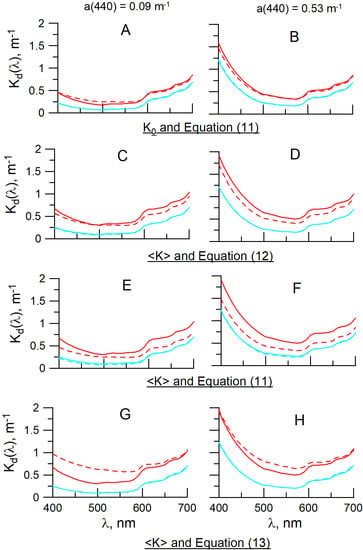
4. Influence of the Coccolithophore Blooms on the Accuracy of the Approximate Formulas

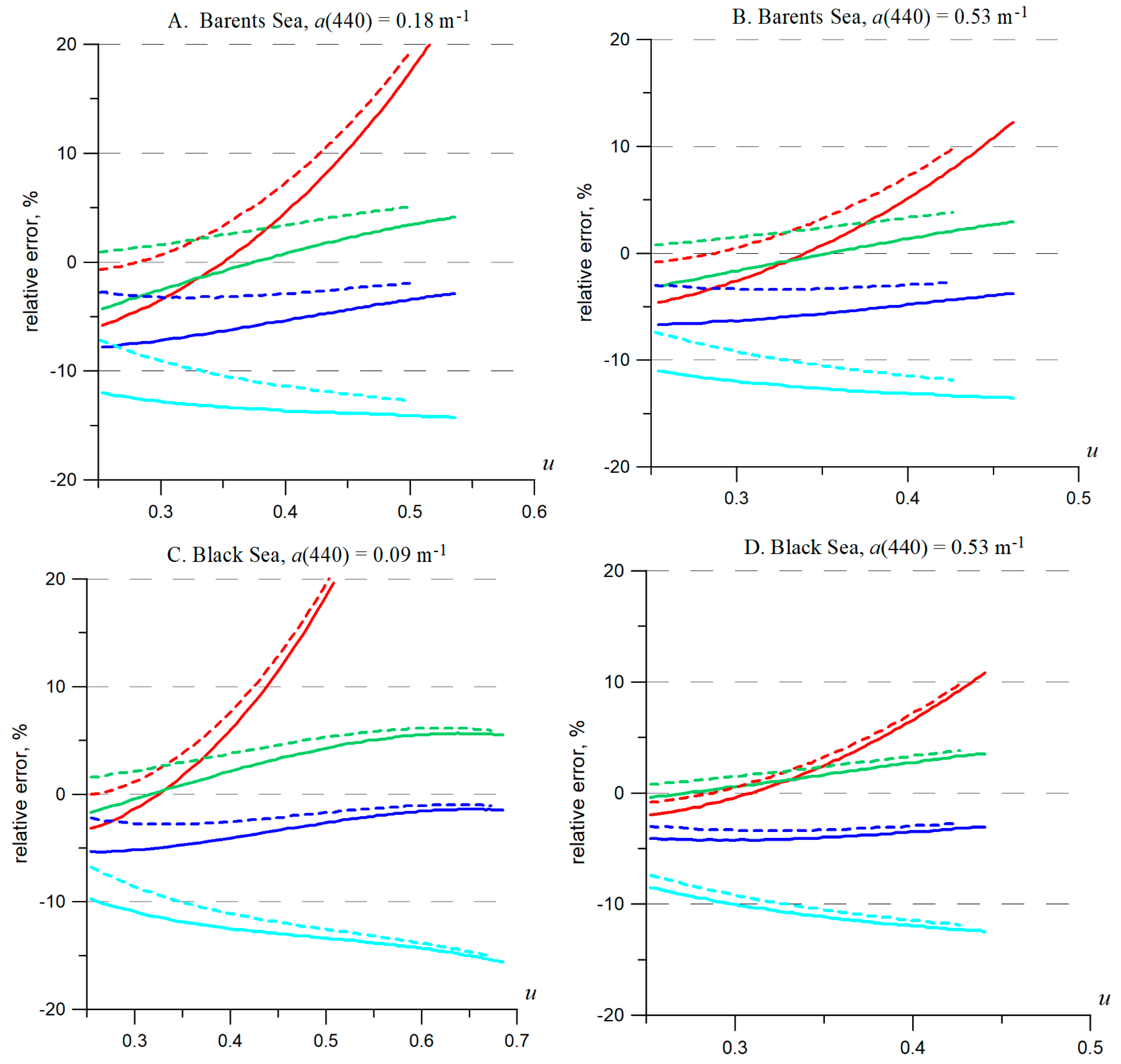
4.1. Water Radiance Reflectance

We tested four approximate formulas [55,56,57,58,59] allowing us to estimate the sub-surface water radiance reflectance ρ(λ) = πLu(λ, 0)/Ed(λ, 0) in terms of the parameter u = bb/(a + bb). The simplest of them [55] was derived by Morel and Gentili for open ocean case 1 waters, u < 0.3.
ρ(u) =π · 0.0922 u/(1 − u)
Lee et al. [56] derived their formula (6) by using the Hydrolight [57,59] simulations for infinitely deep coastal high-scattering water, u < 0.6.
ρ(u) = π (0.070 + 0.155 u0.752) u
Gordon et al. [58] presented their formula for oceanic case 1 waters, u < 0.3.
ρ(u) = π (0.0949 + 0.0794 u) u
Lee et al. [59] modified (9) for both the coastal and open ocean waters, suggesting to use it with other coefficients
ρ(u) = π (0.089 + 0.1245 u) u
Figure 13 shows the plots of ρ(λ), according to Equations (7)–(10) (a similar figure for Equations (7)–(9) was presented in [56]). We see that all Equations (7)–(10) are very close to each other for values u ≤ 0.25 when ρ(λ) ≤ 0.1, a noticeable difference appears only for u ≥ 0.2. For large values of the parameter u, corresponding to the high coccolithophore concentration, Equation (7) gives incredibly large values of ρ; Equations (8) and (10) give similar results; Equation (9) gives the lowest value of ρ, as compared to other formulas.
To assess the applicability of Equations (7)–(10) under the coccolithophore bloom conditions, a numerical simulation of the dependence of ρ on the coccolithophore concentration was made. We have set the acceptable absolute error for ρ equal to 0.01 for ρ ≤ 0.1 (u ≤ 0.25), and the acceptable relative error equal to 10% for ρ > 0.1 or u > 0.25.
It should be noted that all Equations (7)–(10) do not depend on the solar zenith angle θ0. As shown in Section 3.2, a difference between the values of ρ in various atmospheric conditions is quite insignificant. Keeping it in mind, we performed our numerical calculations, intended for the optimal choice between Equations (7)–(10) for the cloudy sky with an optical thickness of cloud τcl = 20, since it gives the value of ρ close to the average for the three considered cases of illumination conditions (clear sky with θ0 = 25° and 60°, and overcast).
Figure 14 presents the relative errors of Equations (7)–(10) as a function of the parameter u for u ≥ 0.25, various values of the absorption coefficient a, taking into account “non-coccolithophore” scattering particles, and without it. We estimated the relative errors of Equations (7)–(10) at 530 nm, performing our numerical simulation for Ncoc from 0 to 107 cell/L. The two upper pictures in Figure 14 correspond to the Barents Sea with the absorption a(440) = 0.18 and 0.53 m1, and the two lower pictures to the Black Sea with a(440) = 0.09 and 0.53 m1 (see Section 2.3).
The values of relative error are shown at the vertical axis (ρappr−ρ)/ρ, where ρ is the result of the numeric simulation and ρappr is calculated by one of the Equations (7)–(10). We took into account the “non-coccolithophore” particles (shown by dashed lines) and the solid lines show the relative errors without “non-coccolithophore” particles. In Figure 14, the minimum value of u = 0.25 corresponds ρ = 0.1, as we set the acceptable relative error (10%) for ρ > 0.1. The maximum values of the parameter u were obtained for Ncoc = 107 cell/L, and they are much larger in the case of low absorption.
It is seen that Equations (8) and (10) result in the acceptable error for all cases under consideration, in contrast to Equations (7) and (9). We explain it by the fact that the Equations (8) and (10) were derived for highly scattering waters. For u < 0.5, the Equation (8) is usually better than (10), for u > 0.5 Equation (10) it is otherwise. It is well seen for the highest u values in the Black Sea in the case of low absorption (Figure 14C). In the case of u < 0.25, all formulas result in 0.01, and all of them are acceptable.
Figure 15 shows the results of comparisons between the spectral values of ρ(λ) obtained by numerical simulation and the estimates by Equations (7)–(10) for the Barents Sea and the Black Sea. In the Black Sea, the numerical simulations were performed with a clear sky and θ0 = 25°, while in the Barents Sea at θ0 = 60°. We calculated the ρ(λ) values for Ncoc = 107 cell/L and low absorption, corresponding to the maximum u values. It is seen in Figure 15 that the values of ρ(λ) by the numerical calculations and Equations (7)–(10) are very close to each other in the case of u ≤ 0.25 for the wavelength λ > 600 nm, the lowest approximation errors are obtained by Equations (8) and (10) for u > 0.25 and λ < 600 nm, and the best approximation for u > 0.5 in the case of the Black Sea, is obtained by Equation (10).
Table 7 presents the absolute and relative errors of Equations (7)–(10) depending on the value of Ncoc and the solar zenith angle for the Black Sea, a(440) = 0.09 m−1 and λ = 490 nm, where the parameter u reaches its maximum value. In the absence of a CB for u = 0.17, the errors of the formulas increase significantly for the large solar zenith angle, but for all formulas, the absolute error does not exceed the threshold value of 0.01.
In the presence of a CB, even one that is not so intensive (Ncoc = 1 × 10⁶ cell/L, u = 0.34), the influence of the solar zenith angle weakens and acceptable values of the relative errors are obtained for the Equations (7), (8) and (10). For Ncoc ≥ 3 and 106 cell/L, u > 0.5 a good approximation and is obtained only by the Equations (8) and (10), regardless of the solar zenith angle.
Summing up the results of our calculations, we can conclude that for u ≤ 0.25, any Equation of (7)–(10) allows us to estimate ρ with an accuracy not worse than 0.01. For u > 0.25, the Equations (8) or (10) give an accuracy not worse than 10%; for u > 0.5, Equation (10) is more reliable.

4.2. Diffuse Attenuation Coefficient

Gordon [54] considered two variants for the diffuse attenuation coefficient Kd. The first case is K0 just beneath the sea surface, the second, <K>, averaged over half of the euphotic zone, corresponding to the optical depth τ10 = 2.3 [54]. In Section 3.3, we calculated both coefficients by using our numerical model and estimated the errors in the downward irradiance Ed(z) obtained by using the exponential law with the constant diffuse attenuation coefficient. In this section, we are estimating the possibility of the use of the approximate formulas for Kd, two of them are Gordon’s formulas [54], the third is developed by Lee et al. [60].
First, Gordon’s formula for K0:
K0 = 1.04 Do (a + bb)
where Do is the parameter of the angular radiance distribution just beneath the surface for a fully absorbing ocean. Do depends on the solar zenith angle θ0, atmospheric conditions (clear or overcast sky), and the wavelength (some results of the computed Do are given in Table 3 [54]). This simple formula is the most often used to calculate Kd through the inherent optical characteristics of seawater.
Gordon’s formula for <K> is a polynomial of the third degree from (1−ω0F):
< K > = c D o   n = 1 3 < k > n ( 1 0 F ) n = c D o   n = 1 3 < k > n [ a + bb c ] n
where F is the forward scattering probability, ω0 is the single scattering albedo, and c is the beam attenuation coefficient; the <k>n coefficients were derived from the results of simulations and its values are given in [54]. For applying Equation (12), we need to know not only the values of a and bb but also the value of c or b. The determining b through bb requires knowing the backscattering probability bb/b determined by the phase scattering function. In the case of a CB, the value of bb/b depends on the wavelength, the CB parameters, and the presence of other optically active components. In our work, we knew the values of bb/b because the phase scattering functions were determined.
Lee et al. [60] present several formulas for <K>, derived from a base of Hydrolight numerical simulations. The simplest of them uses the a and bb coefficients, and the solar zenith angle θ0 as the input parameters
<K> = (1 + 0.005 θ0) a + 3.47 bb
The formula was derived from the simulations with a clear sky, so it cannot be used for cloudy conditions.
Figure 16 and Table 8 present the accuracy estimates for the above formulas depending on the CB intensity in the Black Sea. Figure 16A,B show the applicability of Equation (11) for the estimation of K0. As seen in this case, the errors are practically independent of the CB presence; the average error equals 0.01–0.04 m−1, the maximum is 0.1 m−1. Figure 16C,D demonstrate that the errors of Equation (12) are noticeably larger for Ncoc = 107 cell/L and weakly depend on the absorption spectrum. For an intense CB, Equation (12) underestimates the values of <K> by no more than 0.21 m−1.
As mentioned above, for estimating the attenuation of underwater irradiance with depth, a simpler Equation (11) is often used instead of <K>. Figure 16E,F show that it is acceptable in the absence of a CB, but this formula results in noticeably increasing errors in the case of an intense CB. In this case, Equation (11) underestimates Kd by 0.06–0.21 m−1 (18–33%) for a small a and by 0.17–0.43 m−1 (20–33%) for a large a.
Figure 16G,H show the results of calculations by Equation (13), as compared with numerical calculations. In the absence of a CB, the error of this formula does not exceed 0.03 m−1 (4%), but in the case of Ncoc = 107 cell/L and the absorption value of a(440) = 0.53 m−1, Equation (11) results in overestimated values in the range of 480–590 nm near the absorption minimum, by approximately 0.11–0.16 m−1 (19–30%). For an extreme CB and low absorption (a(440) = 0.09 m−1), the overestimated values are observed in the range 400–590 nm, where the errors reach 0.14–0.34 m−1 (30–110%).
Table 8 presents the absolute errors of the Equations (11)–(13) depending on the Ncoc value, the solar zenith angle θ0, and the absorption coefficient a(440). As seen, all formulas give good results in the absence of a CB. For higher Ncoc values, the errors increase, and only Equations (12) and (13) formulas can provide reasonable results. We can see that in most cases, Equation (12) gives better results for a(440) = 0.09, (11) for a(440) = 0.53. For θ0 = 60°, the Equation (13), including the solar zenith angle θ0 as the input parameter, gives acceptable results for within the whole spectral range for Ncoc = 5⋅106 cell/L and for Ncoc = 107 only for a(440) = 0.53 (for a(440) = 0.09 only for the range of 600–700 nm).
The test results of the accuracy of Equations (11)–(13) for the Barents Sea are similar to the ones obtained for the Black Sea. Figure 17 presents, as an example, the results of comparing the <K> spectra in the Barents Sea (θ0 = 60°) obtained by numerical simulation and by Equations (12) and (13), depending on the value of Ncoc and the absorption coefficient a(440). As in the Black Sea, Equation (12) underestimates the value of <K> for an intense CB, but by a smaller value. For Ncoc = 107 cell/L Equation (12) underestimates <K> by no more than 0.08 m−1 when using the absorption spectrum with a(440) = 0.18 m−1 measured by ICAM and by no more than 0.14 m−1 in the case of the model absorption spectrum with a(440) = 0.53 m−1. As in Table 8, the errors of the Equation (13) are small in the case of a(440) = 0.53 with the exception of Ncoc = 107 cell/L and the spectral range 450–590 nm, where the value of bb is comparable with the value of a (bb ≥ 0.5 a). In the case of a(440) = 0.18 and an intense CB, Equation (13) significantly overestimates <K> for the range of 400–590 nm, also where bb ≥ 0.5 a.
Thus, in the CB case, a choice between Equations (12) and (13) depends on the absorption coefficient value. If the bb value is not too high, compared with the absorption value, it is better to use a simple Equation (13). But this formula results in large errors in the case of low absorption and intense scattering (bb ≥ 0.5 a); in this case, it is better to use Equation (12). However, for its application, knowledge of the bb/b ratio is needed. This raises a problem in its application in the case of remote sensing. The use of Equation (11) is possible only in the CB absence.
For the estimation of the diffuse attenuation coefficient value in the absence of a CB under clear sky conditions, you can use any of Equations (11)–(13); in the case of the cloudy sky, Equations (11) or (12). In the CB case and a clear sky, if the absorption is not too low (bb ≤ 0.5 a), you can use Equation (13). In the case of high scattering and low absorption, you can use Equation (12), if you know the value of bb/b.

5. Discussion and Conclusions

In this section, we will focus on the key issues of our modeling, the choice of a calculation method, forming a set of input parameters, a discussion of one of the most interesting results—the asymptotic regime—and formulate the main conclusions, in particular, the scientific and practical significance of the results.

5.1. Comments to the Calculation Methods

In the Introduction, we considered the most widely used numerical methods: Monte Carlo, DISORT, and Hydrolight. The last seems to be the most appropriate, having a high processing speed and accuracy comparable to Monte Carlo (M-C). But this is a commercial program, rather expensive, and we do not have it. The Monte Carlo method works slowly, but a good agreement with Monte Carlo indicates the reliability of the results. Therefore, we used the modified DISORT for our numerical calculations (see Section 2.2) and M-C for checking the obtained results in selected cases. As an example, we present the results of such a comparison between the underwater radiance calculation by Monte Carlo- and DISORT-based matrix operator methods (Figure 18).

5.2. Set of the Input Parameters

We indicated in Section 2.1 that we did not set out for our modeling to reproduce the results of the field measurements. Still, we needed in situ measured data to approximate the input modeling parameters to the real conditions observed in the Barents Sea and Black Sea. We did not measure all input parameters needed for the calculations, but the measured data allowed us to derive the unmeasured ones (see Table 1).
The choice of appropriate optical characteristics for the main CB components—plated cells and detached coccolites—is particularly difficult due to their complicated shape and noticeable variability depending on external conditions, in particular, on temperature and mineral nutrition. Balch [52] noted “changes in coccolith morphology would cause variability in their backscattering cross-sections, which would translate to changes in their reflectance.” Von Dassow et al. [61] reported about the coccoliths’ ability to rotate linearly polarized light.
Interest in optical characteristics has increased in the last twenty years in connection with the task of quantifying CB parameters from satellite color scanners. In addition to the works [47,48,49,50,51,52] listed in Section 2.3, there are several other publications in which optical parameters were estimated theoretically or from field measurements [62,63,64]. However, the representative set of optical parameters of CB components is only given in the publication [51]. That is the main reason why we took [51] as the base for our numerical calculations. The other reason is the possibility to use the data of [51] for the quantitative assessment of the intensity of coccolithophore blooms in the Barents Sea from satellite data [44].

5.3. Asymptotic Regime

Many researchers have studied the asymptotic regime and derived formulas to describe its angular radiance distribution and calculate the diffuse attenuation coefficient; the interested reader can find the references, including works from the first decade of this millennium, in the books of Kirk [13] and Gordon [21]. All authors agree that the single-scattering albedo, the single-scattering average cosine, and the average square angle are the main parameters determining the features of the asymptotic regime.
We pay attention to the theoretical results presented in [18]. The approach, based on solving the characteristic equation in the small-angle diffusion approximation, allowed the derivation of the formulas for the asymptotic radiance distribution in the range of angles 0°–45° and for estimating the optical depth corresponding to the establishment of the asymptotic regime [18,65]. The examples of estimating such depths for the clearest (1) and turbid coastal (2) waters are presented in [18].
The following parameters were taken at 555 nm: (1) The beam attenuation coefficient c(555) = 0.07 m−1, the single scattering albedo ω0(555) = 0.4, the scattering coefficient b(555) = 0.028 m−1, the average single-scattering cosine <cosθ> = 0.8; (2) 1.0 m−1, 0.9, 0.9 m−1, and 0.48, respectively. The boundary estimates are (1) 23 and 330 m, (2) 60 and 60 m, for the optical and geometrical depth, respectively. It would be interesting to compare these estimates with those obtained from our calculations. As mentioned above, two main conditions determine the asymptotic regime: the angular radiance distribution is symmetrical concerning the vertical axis and unchangeable with depth; The diffuse attenuation coefficient is constant over depth. Table 3 shows the necessary parameters for the depth estimation.
Because we deal with the asymptotic regime, we should set requirements for the accuracy of the fulfillment of the above conditions. As we noted in the Introduction, the advantage of numerical calculations is that their accuracy can be much higher than practically possible in field measurements. We set an accuracy of 3% for the angular distributions and 0.01 m−1 for the diffuse attenuation coefficient k. As can be seen from the Table 3, taking into account the depth discreteness of the presented data, we can accept the following values of the optical and geometrical depth as the boundary of the onset of the asymptotic regime: 6 m and 8 m, respectively, for Ncoc = 5 × 10⁶ cell/L, a(440) = 0.09 and 0.53 m−1, and 5 m for both cases of Ncoc = 107 cell/L. The values of the optical depth for the above boundaries equal 17, 24, 26, and 26, respectively. As compared with the results given in [18], we can note the close values of the optical depths for their clearest case, but the geometrical depths differ by factors of 40–50.
This is an important result from several points of view which have practical significance. In reality, we have a light curtain that creates a significant obstacle for observing underwater objects at shallow depths, as well as for transmitting signals across the surface when using laser communication with underwater objects. On the other hand, we get a natural laboratory, allowing us to study the features of the asymptotic regime in the subsurface layer; the cost of such research, no doubt, is much less than deep-sea research. Such studies can provide a possibility to develop fairly simple methods for evaluating a set of inherent optical characteristics, including the parameters of the phase scattering function.

5.4. Conclusions

The coccolithophore blooms are a planetary-scale phenomenon, a potent producer of CaCO3 in the ocean, affecting the exchange of carbon dioxide between the ocean and atmosphere, the greenhouse effect, and global climate change significantly. We studied the impact of intense coccolithophore blooms on the underwater light fields, which provide the most comprehensive information about the propagation of solar radiation in the water column. We prepared software and the sets of input parameters, corresponding to real conditions in the Barents Sea and Black Sea, for modeling the underwater light fields and their basic parameters under extreme coccolithophore bloom conditions. We used the modified DISORT code and the Monte Carlo method to get the exact data of our numerical calculations. The most interesting of the obtained results comprise data on the asymptotic regime features, whose border of onset can be about five meters as compared with a few hundred meters in the open ocean. This result is of practical significance, denoting an obstacle for observing underwater objects at shallow depths and transmitting the optical signals across the sea surface. On the other hand, we get a natural laboratory, allowing us to study the features of the asymptotic regime near the sea surface. The assessment of the accuracy of the approximating formulas with our exact data enables us to make recommendations for the choice of the optimal algorithm under intensive coccolithophore bloom conditions.

Author Contributions

Conceptualization, O.K.; Formal analysis, S.V.; Investigation, S.V. and S.S.; Methodology, O.K.; Software, S.S.; Writing—original draft, O.K., S.V. and S.S. All authors have read and agreed to the published version of the manuscript.

Funding

This research was supported by RFBR grant № 19-55-45024\19.

Acknowledgments

The results were obtained in the framework of the state assignment of Minobrnauki RF (theme No. 0149-2019-0003). We thank S.I. Pogosyan for a given opportunity to use the ICAM absorption meter in our expeditionary research; V.A. Artemiev, A.V. Grigoriev, A.N. Khrapko for their help in the field studies, V.A. Silkin and L.A. Pautova for providing data of related measurements.

Conflicts of Interest

The authors declare no conflict of interest.

References

  1. Thierstein, H.R.; Young, J.R. Coccolithophores—From Molecular Processes to Global Impact; Springer: Berlin, Germany, 2004. [Google Scholar]
  2. Kopelevich, O.V.; Burenkov, V.I.; Ershova, S.V.; Sheberstov, S.V.; Evdoshenko, M.A. Application of SeaWiFS data for studying variability of bio-optical characteristics in the Barents, Black and Caspian Seas. Deep. Sea Res. Part II Top. Stud. Oceanogr. 2004, 51, 1063–1091. [Google Scholar] [CrossRef]
  3. Kopelevich, O.V.; Burenkov, V.I.; Sheberstov, S.V. Case Studies of optical remote sensing in the Barents Sea, Black Sea, and Caspian Sea. In Remote Sensing of the European Seas; Springer: Dordrecht, Holland, 2008; pp. 53–66. [Google Scholar]
  4. Kopelevich, O.V.; Burenkov, V.I.; Sheberstov, S.V.; Vazyulya, S.V.; Kravchishina, M.D.; Pautova, L.; Silkin, V.A.; Artemiev, V.A.; Grigoriev, V. Satellite monitoring of coccolithophore blooms in the Black Sea from ocean color data. Remote Sens. Environ. 2014, 146, 113–123. [Google Scholar] [CrossRef]
  5. Kopelevich, O.V.; Artemiev, V.A. Comparison of biooptical characteristics of the Baltic, Norwegian, and Barents Seas: Summer 2016 (Cruise 65 of the R/V Akademik Mstislav Keldysh). Oceanology 2017, 57, 340–342. [Google Scholar] [CrossRef]
  6. Kopelevich, O.V.; Vazyulya, S.V.; Grigoriev, A.V.; Khrapko, A.N.; Sheberstov, S.V.; Sahling, I.V. Penetration of visible solar radiation in waters of the Barents sea depending on cloudiness and coccolithophore blooms. Oceanology 2017, 57, 402–409. [Google Scholar] [CrossRef]
  7. Kopelevich, O.V.; Sahling, I.V.; Vazyulya, S.V.; Glukhovets, D.I.; Sheberstov, S.V.; Burenkov, V.I.; Karalli, P.G.; Yushmanova, A.V. Bio-Optical Characteristics of the Seas, Surrounding the Western Part of Russia, from Data of the Satellite Ocean Color Scanners of 1998–2017; OOO «VASh FORMAT»: Moscow, Russia, 2018. [Google Scholar]
  8. Kopelevich, O.V.; Sahling, I.V.; Vazyulya, S.V.; Glukhovets, D.I.; Sheberstov, S.V.; Burenkov, V.I.; Karalli, P.G.; Yushmanova, A.V. Electronic Atlas. Bio-Optical Characteristics of the Seas, Surrounding the Western Part of Russia, from Data of the Satellite Ocean Color Scanners of 1998–2018. Available online: http://optics.ocean.ru/ (accessed on 12 May 2020).
  9. Jerlov, N.G. Marine Optics; Elsevier: Amsterdam, The Netherlands, 1976. [Google Scholar]
  10. Voss, K.J. Electro-optic camera system for measurement of the underwater radiance distribution. Opt. Eng. 1989, 28, 283241. [Google Scholar] [CrossRef]
  11. Timofeeva, V.A. Optics of turbid water. In Optical Aspects of Oceanography; Jerlov, N.G., Nielsen, E.S., Eds.; Academic Press: London, UK, 1974; pp. 177–219. [Google Scholar]
  12. Gershun, A. Light Field; ONTI NKTP: Moscow, Soviet Union, 1936. [Google Scholar]
  13. Gordon, H.R. Physical Principles of Ocean Color Remote Sensing. Available online: https://ioccg.org/wp-content/uploads/2019/11/gordon_book_nov_20_2019.pdf (accessed on 12 May 2020).
  14. Jerlov, N.G. Optical Oceanography; Elsevier: New York, NY, USA, 1968. [Google Scholar]
  15. Ivanoff, A. Introduction a L’oceanographie; Librairie Vuibert: Paris, France, 1975. [Google Scholar]
  16. Ivanov, A.P. Phyzical Background of Hydrooptics; Nauka i technika: Minsk, Soviet Union, 1975. [Google Scholar]
  17. Preizendorfer, R. Hydrologic Optics; NOAA: Honolulu, HI, USA, 1976.
  18. Dolin, L.S.; Levin, I.M. Handbook of the Theory of Underwater Vision; Gidrometeoizdat: Leningrad, Soviet Union, 1991. [Google Scholar]
  19. Monin, A. Ocean Optics; Nauka: Moscow, Soviet Union, 1983. [Google Scholar]
  20. Mobley, C.D. Light and Water: Radiative Transfer in Natural Waters; Academic Press: San Diego, CA, USA, 1994. [Google Scholar]
  21. Kirk, J.T.O. Light and Photosynthesis in Aquatic Ecosystems; Cambridge University Press: Cambridge, UK, 2011. [Google Scholar]
  22. Plass, G.N.; Kattawar, G.W. Monte Carlo calculations of radiative transfer in the earth’s atmosphere–ocean system. 1. Flux in the atmosphere and ocean. J. Phys. Oceanogr. 1972, 2, 139–145. [Google Scholar] [CrossRef] [Green Version]
  23. Jin, Z.; Stamnes, K. Radiative transfer in nonuniformly refracting layered media: Atmosphere-ocean system. Appl. Opt. 1994, 33, 431–442. [Google Scholar] [CrossRef]
  24. Sheberstov, S.V.; Nabiullina, M.V.; Lukyanova, E.A. Numerical modeling of radiative transfer in ocean-atmosphere system with wind-roughened surface. In Proceedings of the II International Conference «Current Problems in Optics of Natural Waters», St. Petersburg, Russia, 8–12 September 2003; pp. 90–95. [Google Scholar]
  25. Mobley, C.D.; Sundman, L.K. Hydrolight 5.2, Ecolight 5.2, Users Guide. Available online: http://www.sequoiasci.com/wp-content/uploads/2013/07/HE52UsersGuide.pdf (accessed on 12 May 2020).
  26. Smyth, T.J.; Moore, G.F.; Groom, S.B.; Land, P.E.; Tyrrell, T. Optical modeling and measurements of a coccolithophore bloom. Appl. Opt. 2002, 41, 7679–7688. [Google Scholar] [CrossRef]
  27. McKee, D.; Cunningham, A.; Craig, S. Semi-empirical correction algorithm for AC-9 measurements in a coccolithophore bloom. Appl. Opt. 2003, 42, 4369–4374. [Google Scholar] [CrossRef] [Green Version]
  28. Tyrrel, T.; Holligan, P.M.; Mobley, C. Optical impacts of oceanic coccoblooms. J. Geophys. Res. Atmos. 1999, 104, 3223–3242. [Google Scholar] [CrossRef]
  29. Glukhovets, D.I.; Kopelevich, O.V.; Sahling, I.V.; Artemiev, V.A.; Pautova, L.A.; Lange, E.K.; Kravchishina, M.D. Biooptical characteristics of the surface layer of the Baltic, Norwegian, and Barents seas in summer 2014–2016 from shipboard and satellite data. Oceanology 2017, 57, 410–418. [Google Scholar] [CrossRef]
  30. Glukhovets, D.I.; Sheberstov, S.V.; Kopelevich, O.V.; Zaytseva, A.F.; Pogosyan, S.I. Measuring the sea water absorption factor using integrating sphere. Light Eng. 2018, 26, 120–126. [Google Scholar] [CrossRef]
  31. Yushmanova, A.V.; Kopelevich, O.V.; Vazyulya, S.V.; Sahling, I.V. Inter-annual variability of the seawater light absorption in surface layer of the northeastern Black Sea in connection with hydrometeorological factors. J. Mar. Sci. Eng. 2019, 7, 326. [Google Scholar] [CrossRef] [Green Version]
  32. Plass, G.N.; Kattawar, G.W.; Catchings, F.E. Matrix operator theory of radiative transfer. 1: Rayleigh scattering. Appl. Opt. 1973, 12, 314–329. [Google Scholar] [CrossRef]
  33. Bates, D.R. Rayleigh scattering by air. Planet. Space Sci. 1984, 32, 785–790. [Google Scholar] [CrossRef]
  34. Gordon, H.R.; Castaño, D.J. Aerosol analysis with Coastal Zone Color Scanner. A simple method for including multiple scattering effects. Appl. Opt. 1989, 28, 1320–1326. [Google Scholar] [CrossRef]
  35. Gordon, H.R.; Wang, M. Surface-roughness considerations for atmospheric correction of ocean color sensors. I: The rayleigh-scattering component. Appl. Opt. 1992, 32, 4247–4260. [Google Scholar] [CrossRef]
  36. Nakajima, T.; Tanaka, M. Effect of wind-generated waves on the transfer of solar radiation in the atmosphere-ocean system. J. Quant. Spectrosc. Radiat. Transf. 1983, 29, 521–537. [Google Scholar] [CrossRef]
  37. Chandrasekhar, S. Radiative Transfer; Dover Publications: New York, NY, USA, 1960. [Google Scholar]
  38. Stamnes, K.; Swanson, R.A. A new look at the discrete ordinate method for radiative transfer calculations in anisotropically scattering atmospheres. J. Atmos. Sci. 1981, 38, 387–398. [Google Scholar] [CrossRef] [Green Version]
  39. Stamnes, K.; Tsay, S.-C.; Wiscombe, W.; Jayaweera, K. Numerically stable algorithm for discrete-ordinate-method radiative transfer in multiple scattering and emitting layered media. Appl. Opt. 1988, 27, 2502–2509. [Google Scholar] [CrossRef]
  40. Kopelevich, O.V. Application of data on seawater light scattering for the study of marine particles: A selective review focusing on Russian literature. Geo Mar. Lett. 2012, 32, 183–193. [Google Scholar] [CrossRef]
  41. Kopelevich, O.V. Low-parameter model of seawater optical properties. In Ocean Optics, Vol. 1: Physical Ocean Optics; Monin, A.S., Ed.; Nauka Pub., Nauka: Moscow, Russia, 1983; Volume 1, pp. 208–234. [Google Scholar]
  42. Levin, I.M.; Kopelevich, O.V. Correlations between the Inherent Hydrooptical Characteristics in the spectral range close to 550 nm. Oceanology 2007, 47, 344–348. [Google Scholar] [CrossRef]
  43. Kopelevich, O.V.; Lutsarev, S.V.; Rodionov, V.V. Spectral absorption by “yellow substance” of ocean waters. Oceanology 1989, 29, 409–414. [Google Scholar]
  44. Kopelevich, O.V.; Burenkov, V.I.; Vazyulya, S.V.; Sheberstov, S.V. Problems of detection of coccolithophore blooms from satellite data. Mod. Probl. Remote Sens. Earth Space 2012, 9, 241–250. [Google Scholar]
  45. Pope, R.M.; Fry, E.S. Absorption spectrum (380–700 nm) of pure water. I. Integrating cavity measurements. Appl. Opt. 1997, 36, 8710–8723. [Google Scholar] [CrossRef]
  46. Burenkov, V.I.; Sheberstov, S.V.; Artemiev, V.A.; Taskaev, V.R. Estimation of measurement error of the seawater beam attenuation coefficient in turbid water of Arctic seas. Light Eng. 2019, 27, 103–111. [Google Scholar] [CrossRef]
  47. Gordon, H.R.; Du, T. Light scattering by nonspherical particles: Application to coccoliths detached from Emiliania huxleyi. Limnol. Oceanogr. 2001, 46, 1438–1454. [Google Scholar] [CrossRef]
  48. Gordon, H.R. Light scattering and absorption by randomly-oriented cylinders: Dependence on aspect ratio for refractive indices applicable for marine particles. Opt. Express 2011, 19, 4673–4691. [Google Scholar] [CrossRef]
  49. Zhai, P.-W.; Hu, Y.; Trepte, C.R.; Winker, D.M.; Josset, D.B.; Lucker, P.L.; Kattawar, G.W. Inherent optical properties of the coccolithophore: Emiliania huxleyi. Opt. Express 2013, 21, 17625–17638. [Google Scholar] [CrossRef]
  50. Reynolds, R.A.; Stramski, D.; Neukermans, G. Optical backscattering by particles in Arctic seawater and relationships to particle mass concentration, size distribution, and bulk composition. Limnol. Oceanogr. 2016, 61, 1869–1890. [Google Scholar] [CrossRef] [Green Version]
  51. Voss, K.J.; Balch, W.M.; Kilpatrick, K.A. Scattering and attenuation properties of emiliania huxleyi cells and their detached coccoliths. Limnol. Oceanogr. 1998, 43, 870–876. [Google Scholar] [CrossRef] [Green Version]
  52. Balch, W.M. The ecology, biogeochemistry, and optical properties of coccolithophores. Annu. Rev. Mar. Sci. 2018, 10, 71–98. [Google Scholar] [CrossRef]
  53. Algorithm Descriptions. Available online: https://oceancolor.gsfc.nasa.gov/atbd/ (accessed on 16 May 2020).
  54. Gordon, H.R. Can the Lambert-Beer law be applied to the diffuse attenuation coefficient of ocean water? Limnol. Oceanogr. 1989, 34, 1389–1409. [Google Scholar] [CrossRef]
  55. Morel, A.; Gentili, B. Diffuse reflectance of oceanic waters. Bidirectional aspects. Appl. Opt. 1993, 32, 6864–6879. [Google Scholar] [CrossRef] [PubMed]
  56. Lee, Z.; Carder, K.L.; Mobley, C.D.; Steward, R.G.; Patch, J.S. Hyperspectral remote sensing for shallow waters. I. A semianalytical model. Appl. Opt. 1998, 37, 6329–6338. [Google Scholar] [CrossRef] [PubMed]
  57. Mobley, C.D.; Gentili, B.; Gordon, H.R.; Jin, Z.; Kattawar, G.W.; Morel, A.; Reinersman, P.; Stamnes, K.; Stavn, R.H. Comparison of numerical models for computing underwater light fields. Appl. Opt. 1993, 32, 7484–7504. [Google Scholar] [CrossRef] [Green Version]
  58. Gordon, H.R.; Brown, O.B.; Evans, R.H.; Brown, J.W.; Smith, R.C.; Baker, K.S.; Clark, D.K. A semianalytic radiance model of ocean color. J. Geophys. Res. Space Phys. 1988, 93, 10909–10924. [Google Scholar] [CrossRef]
  59. Lee, Z.; Carder, K.L.; Arnone, R.A. Deriving inherent optical properties from water color: A multiband quasi-analytical algorithm for optically deep waters. Appl. Opt. 2002, 41, 5755–5772. [Google Scholar] [CrossRef]
  60. Lee, Z.-P.; Du, K.-P.; Arnone, R. A model for the diffuse attenuation coefficient of downwelling irradiance. J. Geophys. Res. 2005, 110, 02016. [Google Scholar] [CrossRef]
  61. von Dassow, P.; Engh, G.; Iglesias-Rodrıguez, M.D.; Gittins, J.R. Calcification state of coccolithophores can be assessed by light scatter depolarization measurements with flow cytometry. J. Plankton Res. 2012, 34, 1011–1027. [Google Scholar] [CrossRef] [Green Version]
  62. Fournier, G.; Neukermans, G. An analytical model for light backscattering by coccoliths and coccospheres of Emiliania huxleyi. Opt. Express 2017, 25, 14996. [Google Scholar] [CrossRef] [PubMed]
  63. Hovland, E.K.; Hancke, K.; Alver, M.O.; Drinkwater, K.; Høkedal, J.; Johnsen, G.; Moline, M.; Sakshaug, E. Optical impact of an emiliania huxleyi bloom in the frontal region of the Barents Sea. J. Mar. Syst. 2014, 130, 228–240. [Google Scholar] [CrossRef] [Green Version]
  64. Poulton, A.J.; Young, J.R.; Bates, N.R.; Balch, W.M. Biometry of detached emiliania huxleyi coccoliths along the Patagonian Shelf. Mar. Ecol. Prog. Ser. 2011, 443, 1–17. [Google Scholar] [CrossRef] [Green Version]
  65. Dolin, L.S. Propagation of a narrow beam of light in a medium with strongly anisotropic scattering. Radiophys. Quantum Electron. 1967, 9, 40–47. [Google Scholar] [CrossRef]
Figure 1. The basic instruments for field measurements. Photos captured by A.V. Grigoriev (AD,F) and D. I. Glukhovets (E), both from the Shirshov Institute of Oceanology (SIO RAS) used here with permission.
Jmse 08 00456 g001
Figure 2. The phase scattering function: (A) For the plated cell and coccolith; (B) For the non-coccolithophore particles in the Black Sea (red curve) and the Barents Sea (blue).
Jmse 08 00456 g002
Figure 3. Spectral values of the absorption coefficient (A,B) and the backscattering coefficient depending on the Ncoc (106 cell/L) concentration (C,D): A, C, the Black Sea; B, D, the Barents Sea. The curves 1 and 2 in Figures A and B relate to two values of the seawater absorption coefficient: A, a(440) = 0.09 m−1 and 0.53 m−1, respectively; B, 0.18 and 0.53 m−1, respectively.
Jmse 08 00456 g003
Figure 4. Black Sea. The radiance distributions in the plane of the sun as a function of the viewing angle θ (the range of positive values of θ corresponds to the azimuthal viewing angle ϕ = 0°, the negative values ϕ = 180°; the downward radiance in the θ range of and −90° ÷ +90°, the upward radiances −180° ÷ (−90°) and 90° ÷ 180°). The left part shows the absorption a(440) = 0.09 m−1, the right, a(440) = 0.53 m−1. The numbers near the curves show the depth in meters. For θ0 = 25°, λ = 530 nm, wind speed 0 m/s.
Jmse 08 00456 g004
Figure 5. Barents Sea. The same as in Figure 4. (A) Ncoc = 0 cell/L, a(400) = 0.18 m−1; further respectively. (B) 0, 0.53; (C) 5 × 10⁶, 0.18; (D) 5 × 10⁶, 0.53; (E) 107, 0.18; (F) 107, 0.53; θ0 = 60°.
Jmse 08 00456 g005
Figure 6. Black Sea. The angular radiance distributions for different observation conditions. On the left, the solar zenith viewing angle θ0 = 60°, on the right, overcast condition. All others are the same as in Figure 4.
Jmse 08 00456 g006
Figure 7. Black Sea. Comparison of the radiance distributions for cases of smooth and rough surfaces; a(440 ) = 0.09 m−1, θ0 = 25°, λ = 530 HM, Ncoc = 5 106 cell/L. All others are the same as in Figure 4.
Jmse 08 00456 g007
Figure 8. Black Sea. The angular radiance distributions at 410 and 670 nm; a(440) = 0.09 m−1, θ0 = 25°, wind speed 0 m/s. All others are the same as in Figure 4.
Jmse 08 00456 g008
Figure 9. The spectra of the radiance reflectance as a function of the concentration of coccolithophores for the Black Sea (A,B) and the Barents Sea (C,D); the values of the absorption coefficient a(440) equal A, 0.09 m−1, B, 0.53 m−1, C, 0.18 m−1, D, 0.53 m−1. For the Black Sea, solid lines, θ0 = 25°; dashed lines, θ0 = 60°; for the Barents Sea, solid lines, θ0 = 60°; dashed lines, overcast. The numbers near the curves indicate Ncoc, 106 cell/L.
Jmse 08 00456 g009
Figure 10. The downward irradiance profiles calculated for the case of the Black Sea, λ = 500 nm and θ0 = 25°, depending on the coccolithophore concentration Ncoc for the absorption coefficient a(440) = 0.09 m−1 (a) and 0.53 m−1 (b). The numbers near the curves indicate the Ncoc, 106 cell/L values.
Jmse 08 00456 g010
Figure 11. The downward irradiance Ed(500) profiles for the case of the Black Sea and θ0 = 25°, depending on the coccolithophore concentration (Ncoc = 0, blue curves; Ncoc = 5 × 10⁶ cell/L, magenta) and the absorption coefficient (on (a) with a(440) = 0.09 m−1, on (b), 0.53 m−1). The solid line shows the results of numerical simulation, the dotted line shows calculation for Kd = K0 = const.
Jmse 08 00456 g011
Figure 12. The results of model simulation of the diffuse attenuation coefficient <K> for the photic layer as a function of Ncoc (106 cell/L) and the absorption coefficient a(440). The cases (A,B) are calculated for the Black Sea and θ0 = 25°; (C,D) For the Barents Sea and θ0 = 60°.
Jmse 08 00456 g012
Figure 13. Functions ρ(λ) according to Equations (7)–(10). Red line, Equation (7); Green, Equation (8); light blue, Equation (9); Blue, Equation (10).
Jmse 08 00456 g013
Figure 14. Relative errors of Equations (7)–(10), depending on the parameter u, taking into account the “non-coccolithophore” particles (dashed lines) and without it (solid lines). The color of the curves is the same as in Figure 13.
Jmse 08 00456 g014
Figure 15. Spectral values of ρ(λ) obtained for Ncoc = 107 cell/L by numerical simulation (black curves) and by using approximate formulas (the color of the curves corresponds to Figure 13), in comparison with parameter u (dashed purple lines and right axis). (A) Black Sea, a(440) = 0.09 m−1, θ0 = 25°; (B) Barents Sea, a(440) = 0.18 m−1, θ0 = 60°.
Jmse 08 00456 g015
Figure 16. Spectral values of the diffuse attenuation coefficient Kd in the Black Sea, θ0 = 25°, Ncoc = 107 cell/L (red curves) and Ncoc = 0 (blue curves), a(440) = 0.09 m−1 (left column) and 0.53 m−1 (right column). The cases (A,B) are calculated for K0, the all others for <K>; solid lines, by numerical calculations; dashed lines, with the approximated Equations; (A,B) and (E,F), Equation (11), (C,D), Equation (12), (G,H), Equation (13).
Jmse 08 00456 g016
Figure 17. Spectral values of the diffuse attenuation coefficient <K> depending on the Ncoc (106 cell/L), clear sky, θ0 = 60°. Solid lines, numerical simulation; dashed curves, the approximate formulas. (A,C), ICAM absorption a(440) = 0.18 m−1; (B,D), the modeling absorption a(440) = 0.53 m−1. (A,B), Equation (12); C, D, Equation (13).
Jmse 08 00456 g017
Figure 18. Comparison between the radiance calculation results by Monte Carlo and discrete ordinate methods. Coccolithophore concentration 5⋅106 cell/L, wavelength 410 nm, depths 0 and 4 m. Red and blue lines present the Monte Carlo results; black and green, matrix operator method.
Jmse 08 00456 g018
Table 1. Measured and derived parameters 1 for modeling.
Seawater Optical
Parameters
absorption coefficients: seawater—a(λ), filtrate—af(λ),
CDOM—ag(λ) = af(λ)−aw(λ), particulate—ap(λ);
Beam attenuation coefficient—c(530);
Scattering coefficient—b(530) = c(530)−a(530);
Backscattering coefficient—bb(λ) from ρ(λ);
b(λ), β(λ), P(λ)—using model [40,41,42,43]
Coccolithophore
Parameters
plated cell and coccolith concentration Ncoc and Nlith—from direct determination or by setting for model;
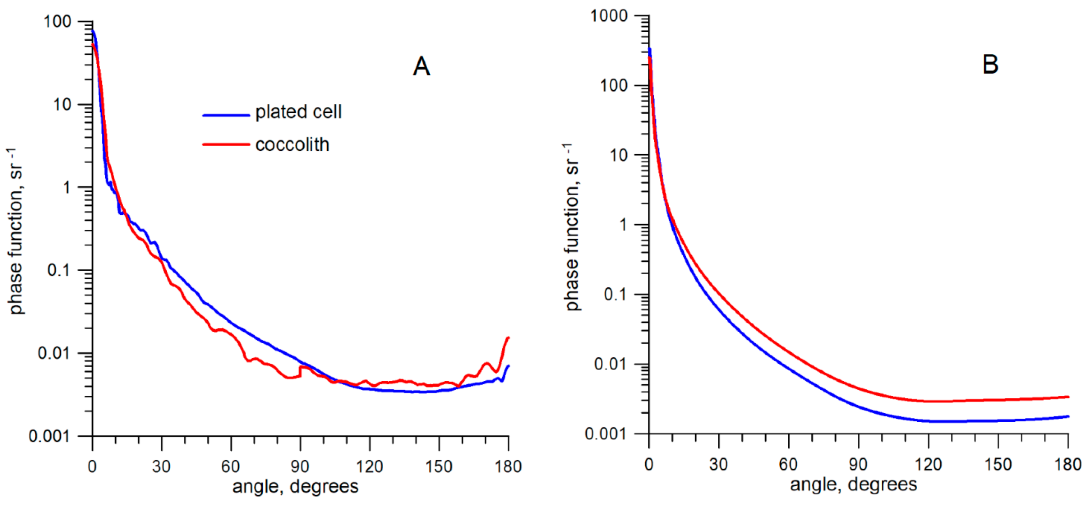
Optical characteristics—from [4,44].
Non-coccolithophore Parametersparticle scattering coefficients bp(λ), βp(λ), Pp(λ)—using model [40,41,42,43];
absorption coefficient from ICAM measurements as a(λ)−aw(λ) or by setting for model;
1 the inherent seawater characteristics are assumed to be independent from depth.
Table 2. Set of optical characteristics * for the modeling.
Input ParametersOptical Characteristics
Ncoca(440)b(440)ω0(440)b(555)bb(555)ω0(555) b ˜ b ( 555 ) <cos>
Black Sea
00.090.600.870.480.0080.8640.0170.922
00.530.600.5310.480.0080.7480.0170.922
50.093.820.9772.810.0750.9740.0270.895
50.533.780.8772.810.0750.9450.0270.895
100.096.830.9875.130.1410.9850.0270.892
100.536.930.9295.130.1410.9690.0270.892
Barents Sea
00.182.550.9342.180.020.9430.00910.949
00.532.530.8272.180.020.930.00910.949
50.185.630.9694.370.0820.9710.01880.918
50.535.560.9134.370.0820.9640.01880.918
100.188.390.9796.560.1450.9850.02210.908
100.538.610.9426.560.1450.9750.02210.908
* Ncoc, the coccolithophore concentration, 106 cell/L; a(440), the seawater absorption coefficient at 440 nm, m−1; b(555) and bb(555), the total scattering and backscattering coefficients at 555 nm, m−1; ω0(440) and ω0(555), the single scattering albedo at 440 and 550 nm (non-dimensional); b ˜ b ( 555 ) ,   the backscattering probability; <cos>, the average cosine of the single scattering (non-dimensional)
Table 3. Normalized angular distributions of underwater radiance in the Black Sea and Barents Sea.
Black Sea
Ncoc = 5 × 10⁶ cell/L, a(440) = 0.09 m−1Ncoc = 5 × 10⁶ cell/L, a(440) = 0.53 m−1
z, m−90−4504590k *z, m−90−4504590k
40.9101.4912.3661.9491-40.8672.0234.0332.8811
60.9671.6802.3011.84410.28160.9462.3663.9752.70810.485
100.9961.7772.2921.79510.264100.9932.5703.9862.61610.471
141.0001.7882.2931.79010.260140.9992.5983.9932.60410.467
Ncoc = 107 cell/L, a(440) = 0.09 m−1Ncoc = 107 cell/L, a(440) = 0.53 m−1
z, m−90−4504590kz, m−90−4504590k
40.9901.4991.8311.5471-40.9811.9562.7462.0571
60.9991.5271.8301.53210.35060.9982.0152.7482.02910.608
81.0001.5301.8301.53110.34881.0002.0232.7502.02510.605
101.0001.5301.8311.53010.349101.0002.0242.7502.02410.605
Barents Sea
Ncoc = 5 × 10⁶ cell/L, a(440) = 0.18 m−1Ncoc = 5 × 10⁶ cell/L, a(440) = 0.53 m−1
z, m−90−4504590kz, m−90−4504590k
40.8861.7562.6852.3761-40.8721.9363.1562.6911
60.9692.0292.9042.19410.40660.9642.2683.4462.47510.485
100,9961,7772,2921,79510.417100.9972.3993.5292.41410.497
141.0001.7882.2931.79010.418141.0002.4093.5342.41010.499
Ncoc = 107 cell/L, a(440) = 0.18 m−1Ncoc = 107 cell/L, a(440) = 0.53 m−1
z, m−90-4504590kz, m−90−4504590k
40.9771.7552.2901.8241-40.9830.9832.6182.0061
60.9991.7962.3111.80310.52560.9980.9982.6471.98010.621
81.0001.8002.3131.80110.52681.0001.0002.6491.97710.620
101.0001.8012.3131.80110.526101.0001.0002.6491.97610.623
* k (m−1) is the diffuse attenuation coefficient in the asymptotic regime.
Table 4. The changes in the ratio ρ(490)/ρ(550) depending on the Ncoc concentration.
Ncoc, 106 cell/L013510
Black Sea, a(440) = 0.09 m−1, θ0 = 25°1.91.71.51.41.3
Black Sea, a(440) = 0.53 m−1, θ0 = 25°0.870.820.820.830.86
Barents Sea, a(440) = 0.18 m−1, θ0 = 60°1.101.081.061.051.04
Barents Sea, a(440) = 0.53 m−1, θ0 = 60°0.820.810.820.840.82
Table 5. The depth of the photic layer Z1% (m) for λ = 500 nm, in the cases of the Black Sea and Barents Sea, depending on the value of Ncoc, the illumination conditions, and the absorption coefficient.
Ncoc, 106 cell/L05100510
Illumination ConditionsBlack Sea, a(440) = 0.09 m−1Black Sea, a(440) = 0.53 m−1
Clear Sky,θ0 = 25°>4020.815.616.39.27.1
Clear Sky,θ0 = 60°>4020.215.214.48.76.8
Overcast>4020.515.515.69.07.0
Illumination ConditionsBarents Sea, a(440) = 0.18 m−1Barents Sea, a(440) = 0.53 m−1
Clear Sky,θ0 = 25°17.510.88.513.18.56.8
Clear Sky,θ0 = 60°16.310.48.312.18.16.5
Overcast17.010.68.412.78.46.7
Table 6. The value of <K> (500) m−1 for the cases of the Black Sea and Barents Sea, depending on the value of Ncoc, illumination conditions, and the absorption coefficient.
Ncoc, 106 cell/L05100510
Illumination ConditionsBlack Sea, a(440) = 0.09 m−1Black Sea, a(440) = 0.53 m−1
Clear Sky, θ0 = 25°0.0940.2240.3040.2720.4870.639
Clear Sky, θ0 = 60°0.1050.2360.3170.3170.5320.684
Overcast0.0980.2280.3090.2880.5030.656
Illumination ConditionsBarents Sea, a(440) = 0.18 m−1Barents Sea, a(440) = 0.53 m−1
Clear Sky, θ0 = 25°0.2520.4110.5250.3350.5200.661
Clear Sky, θ0 = 60°0.2840.4440.5580.3850.5690.705
Overcast0.2630.4230.5380.3540.5380.675
Table 7. Absolute and relative errors of Equations (7–10), depending on the Ncoc value and the solar zenith angle for the Black Sea, λ = 490 nm and a(440) = 0.09 m−1. The value of parameter u is shown in the first column in brackets.
Ncoc, 106 Cells/Lθ0, °Absolute Formula ErrorsRelative Formula Errors
(7)(8)(9)(10)(7)(8)(9)(10)
0
(0.17)
25−0.004−0.004−0.005−0.004−6%−6%−8%−6%
60−0.008−0.008−0.010−0.009−12%−12%−14%−13%
1
(0.34)
250.0020.001−0.017−0.0071%1%−12%−5%
60−0.004−0.005−0.023−0.013−3%−3%−15%−8%
3
(0.53)
250.0640.014−0.035−0.00424%5%−13%−2%
600.0590.009−0.039−0.00922%4%−15%−3%
5
(0.63)
250.170.021−0.049−0.00349%6%−14%−1%
600.160.018−0.052−0.00648%5%−15%−2%
10
(0.77)
250.500.020−0.080−0.011109%4%−18%−2%
600.500.021−0.079−0.009109%5%−17%−2%
Table 8. The absolute errors (m−1) of the Equations (11–13) for determining <K>, depending on the value of Ncoc (106 cell/L), the solar zenith angle θ0 (°), and the absorption coefficients a(440), m−1.
a(440)0.090.53
θ025602560
λ, nm(13)(12)(11)(13)(13)(12)(11)(13)
Ncoc = 0
400−0.004−0.010−0.032−0.0020.018−0.0080.0320.039
450−0.002−0.012−0.029−0.0040.006−0.001−0.007−0.001
500−0.001−0.012−0.024−0.0030.000−0.001−0.019−0.009
550−0.003−0.007−0.021−0.007−0.0010.000−0.017−0.010
6000.0040.004−0.011−0.0100.0070.004−0.007−0.010
6500.0110.005−0.001−0.0100.0130.0040.001−0.010
7000.0290.0010.017−0.0090.0300.0010.018−0.009
Ncoc = 5
4000.11−0.09−0.160.11−0.001−0.08−0.220.01
4500.13−0.05−0.100.130.02−0.09−0.190.01
5000.13−0.03−0.070.130.05−0.08−0.150.04
5500.09−0.05−0.080.090.05−0.07−0.120.04
6000.03−0.07−0.130.010.02−0.07−0.130.002
6500.01−0.05−0.12−0.010.01−0.05−0.12−0.01
7000.02−0.03−0.11−0.030.02−0.03−0.11−0.03
Ncoc = 10
4000.30−0.11−0.200.300.04−0.20−0.430.05
4500.33−0.03−0.100.330.11−0.17−0.310.10
5000.32−0.004−0.060.310.16−0.12−0.210.16
5500.23−0.04−0.100.230.15−0.10−0.180.14
6000.10−0.11−0.190.080.08−0.12−0.210.06
6500.06−0.11−0.210.030.05−0.11−0.210.02
7000.03−0.09−0.21-0.020.03−0.09−0.21−0.02

