Monthly and Quarterly Sea Surface Temperature Prediction Based on Gated Recurrent Unit Neural Network

Abstract

The sea surface temperature (SST) is an important parameter of the energy balance on the Earth’s surface. SST prediction is crucial to marine production, marine protection, and climate prediction. However, the current SST prediction model still has low precision and poor stability. In this study, a medium and long-term SST prediction model is designed on the basis of the gated recurrent unit (GRU) neural network algorithm. This model captures the SST time regularity by using the GRU layer and outputs the predicted results through the fully connected layer. The Bohai Sea, which is characterized by a large annual temperature difference, is selected as the study area, and the SSTs on different time scales (monthly and quarterly) are used to verify the practicability and stability of the model. The results show that the designed SST prediction model can efficiently fit the results of the real sea surface temperature, and the correlation coefficient is above 0.98. Regardless of whether monthly or quarterly data are used, the proposed network model performs better than long short-term memory in terms of stability and accuracy when the length of the prediction increases. The root mean square error and mean absolute error of the predicted SST are mostly within 0–2.5 °C.

1. Introduction

The sea surface temperature (SST) is an important parameter of the energy balance on the Earth’s surface, and it plays a fundamental role in energy, momentum, and water exchange between the ocean and atmosphere [1,2,3]. SST changes have an immeasurable effect on global climate and biological systems [4,5,6]. Therefore, the timely prediction of SST is crucial in many application fields, such as climate prediction, marine fishery production, and marine environmental protection [7,8,9]. However, the prediction accuracy is unsatisfactory due to the influence of many uncertain factors, such as heat flux, radiation, and diurnal wind near the sea surface [10].

At present, SST prediction is mainly divided into physics-based numerical prediction [11,12] and data-driven prediction methods. The former achieves SST prediction by modeling the physical environment. The accuracy of this method depends on the degree of refinement of the model parameters. The more refined the physical environment parameters, the higher the prediction accuracy; however, various problems, such as increased computational complexity and difficulty in obtaining many parameters, also emerge. The seasonal prediction based on a physics-based numerical model has satisfactory performance and prediction accuracy, but it performs poorly for the prediction of long time-series data at a smaller scale. Data-driven prediction methods have gradually developed into traditional statistical methods, machine learning, and artificial neural network learning algorithms. Traditional statistical methods include regression analysis [13], Markov model [14] and harmonic analysis [15]. Although these methods can predict the trend of SST to a certain extent, the overall prediction accuracy is low, and the length of prediction time is limited. When the forecast length is nine in the monthly data, these values basically reach their maximum prediction length. Shallow machine learning methods, such as the support vector machine [16,17] and genetic algorithm [18,19], have been applied to SST prediction. These methods can avoid the multiple minima problem associated with nonlinear optimization and have better prediction accuracy than the traditional prediction method. However, the performance of these machine learning methods depends on a set of parameters that appear in the related learning problem. In this way, the choice of appropriate values is a difficult task that demands the application of structured methods.

With the continuous innovation of deep learning techniques and algorithms, these methods have been widely used in SST prediction because of their powerful learning and modeling capabilities [20,21]. The recurrent neural network (RNN) can effectively manage time series, but when it processes long time-series data, a serious problem of gradient disappearance or explosion arises. Long short-term memory (LSTM) is a special recursive neural network that can preserve and remove data information by adding “gate” settings and a “cell state” to solve the gradient explosion or disappearance of back propagation. The approach has been proven to perform better in processing time data than RNN [22]. LSTM can avoid the problem of gradient explosion and dissipation and solve the problem of long-term dependence. The root mean square error (RMSE) of the daily data for a prediction length of 30 days is within 1.2 °C. The CFCC–LSTM (combined full convolution LSTM and convolution neural network) model is an end-to-end spatiotemporal sequence prediction method which was proposed by Yang [23] on the basis of LSTM. The spatial information of the image sequences can be considered in this CFCC-LSTM model to improve the prediction performance. The RMSE of daily data for a prediction length of 30 days is within 0.75 °C, which is obviously better than LSTM. Besides, to decrease the prediction error of the LSTM model, some scholars use a hybrid mechanism combining different models to predict time-series data and achieve improved results [24,25,26]. However, problems of over-fitting and under-fitting remain due to the high network complexity. The gated recurrent unit (GRU) [27] is a variant of LSTM that maintains the advantages of LSTM for memorizing long-term sequences while simplifying the structure, reducing the training parameters, and alleviating the over and under-fitting phenomena of the network. Although GRU has played a role in acoustic feature extraction [28], network security [29], text information extraction [30] and other fields, to the best of our knowledge, this study is the first to attempt to use GRU to solve the problem of SST prediction.

The main contributions of this paper are the following: (1) a fully connected neural network model based on GRU is designed to predict SST with high accuracy over the medium and long term. This model uses the GRU layer to capture the SST time regularity and the fully connected layer to output the prediction results; (2) the effectiveness and stability of the proposed method are verified by selecting a sea area with a large temperature fluctuation and conducting prediction tests on the SST product data of remote sensing radiometers with long time-series on monthly and quarterly time scales.

The remainder of this article is organized as follows: Section 2 describes the study area and time-series SST data obtained from the satellite used in this study. Section 3 presents the proposed network model for SST prediction. Section 4 provides the experimental results and discussion. Finally, Section 5 summarizes the paper.

2. Materials and Methods

2.1. Study Area

Testing the stability and validity of the prediction algorithm to ensure that the annual temperature fluctuation varies greatly is an important consideration. The Bohai Sea is located northeast of China, between latitude 37°07′ N–40°56′ N and longitude 117°33′ E–122°08′ E. The eastern side of the Bohai Sea is adjacent to the Yellow Sea, by the boundary between the Laotie Mountain of the Liaodong Peninsula and the Penglai Mountain at the northern end of the Shandong Peninsula; the other three sides are surrounded by land. The Bohai Sea has the largest temperature difference and highest latitude of the four seas in China. Therefore, this study uses the Bohai Sea, with large temperature changes, as the study area. From this sea area, six sites are selected for prediction research. Figure 1 shows the study area.

2.2. Data Source

The U.S. National Oceanic and Atmospheric Administration 1/4° daily Optimum Interpolation (OISST) is used in this study. This resource contains a global grid SST formed by combining observation data from different platforms, such as satellites, ships, and buoys. The OISST dataset consists of two types of data, namely from the Advanced Very-High-Resolution Radiometer (AVHRR) and Advanced Microwave Scanning Radiometer for the Earth Observing System (AMSR-E). Since the AMSR-E stopped working in October 2011, the AVHRR-only dataset with a longer time series than AMSR-E was adopted in this study. The dataset covers the global daily SST values from 89.975°S to 89.875°N and 0.125°E to 359.875°E from September 1, 1981 to the present. This study selects the site data from January 1982 to December 2019 and reorganizes the data on the basis of the monthly and seasonal averages. Therefore, each site from P1 to P6, as shown in Figure 1, generates 456 items of monthly data from January 1982 to December 2019 and 152 items of quarterly data from spring 1982 to winter 2019.

Table 1. Statistics of the sea surface temperature (SST) time series at P1 to P6 from Januaray 1982 to December 2019 (the unit is °C).

Site	Month				Quarter
	Mean	Coldest	Warmest	Std.dev	Coldest	Warmest	Std.dev
P1	13.12	−0.44	27.05	8.48	2.18	24.09	7.69
P2	12.99	0.22	26.51	8.16	2.65	23.13	7.46
P3	13.59	−0.31	28.59	8.90	1.83	26.06	8.09
P4	12.86	−0.22	26.57	8.33	2.11	23.36	7.62
P5	13.13	0.66	26.79	7.86	3.13	23.21	7.19
P6	12.53	0.26	25.82	7.95	2.75	22.66	7.29

The headings “Mean”, “Coldest”, and “Warmest” represent the mean value, minimum value, and maximum value for monthly or quarterly data, respectively. Std.dev represents the standard deviation for monthly or quarterly data. There is no subitem “Mean” for quarter data in Table 1 because the mean values of all quarterly data are the same as those of monthly data, which are the average temperature of the region for 38 years. Thus, in order to avoid duplication, only the means of monthly data are shown in the table.

shows the basic statistical characteristics of the data used in the experiments.

3. Methods

A neural network model for the high-precision prediction of medium and long-term SSTs based on GRU and a fully connected layer is constructed. The sequential prediction of the time series of SST data is performed by observing and learning the regular characteristics of historical data over a certain time window. The time window is moved forward to make predictions for the next time node until all training data have been covered. The number of trainings can be set to repeat this learning process, enhancing the accuracy and generalization of the predictive model.

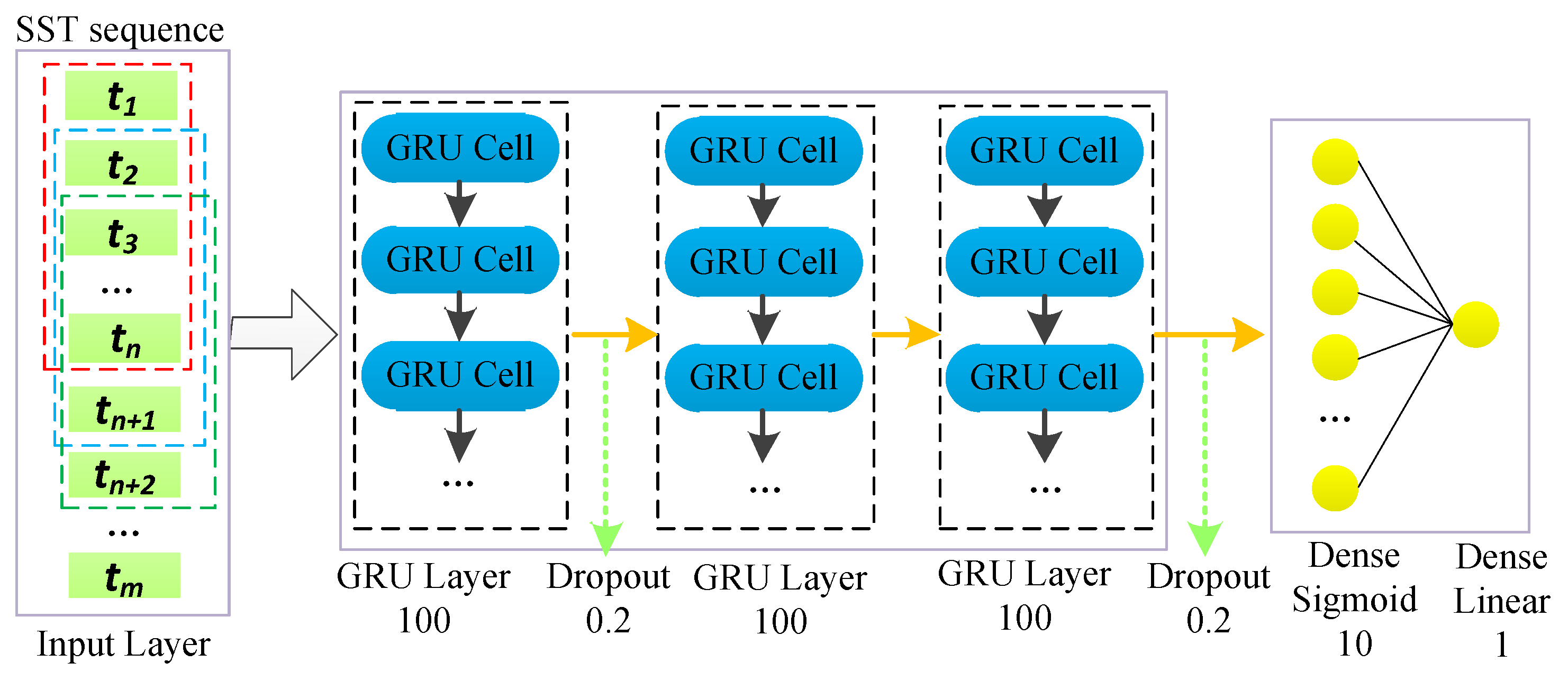
3.1. GRU Neural Network Model

GRU is a variant of LSTM. LSTM adds three gate functions on the basis of the RNN network, namely the input, forgetting, and output gates to the control input, memory, and output values, respectively. However, only two gates are present in the GRU model: update and reset gates. Figure 2 presents the specific structure, where σ is the gating function.

GRU combines the forgetting and input gates of LSTM into a single update gate. This process effectively reduces the amount of calculation and the probability of gradient explosion or disappearance. The specific working mechanism is as follows [27]:

$$Z_t=\mathsf{\sigma }\left(W_z·\left[h_{t-1},x_t\right]+b_z\right),$$

(1)

$$r_t=\mathsf{\sigma }\left(W_r·\left[h_{t-1},x_t\right]+b_r\right),$$

(2)

$$h_t^{\prime }=tanh\left(W·\left[r_t\ast h_{t-1},x_t\right]+b_h\right),$$

(3)

$$h_t=(1-z_t)\ast h_{t-1}+z_t\ast h_t^{\prime },$$

(4)

$$y_t=\mathsf{\sigma }\left(W_0·h_t\right),$$

(5)

where Z_t and r_t represent the update and reset gates, respectively. $W_z$, $W_r$, $W$, and W are the weight parameters of the input data, $h_{t-1}$ is the output of the previous layer, and $x_t$ is the input of the current layer. $b_z$, $b_r$, and $b_h$ are the biases, $\sigma$ is the sigmoid function, and tanh is used to help adjust the value flowing through the network. The output values after $\sigma$ and tanh functions are controlled between (0, 1) and (−1, 1), respectively.

After obtaining the final output, the loss value can be calculated by the loss function:

$$E_t=\frac{1}{2}{\left(y_d-y_t^0\right)}^2,$$

(6)

$$E={{\displaystyle \sum }}_{t=1}^T{E}_t,$$

(7)

where E_t is the loss of a single sample at a certain time, $y_d$ is the real label data, $y_t^0$ is the output value of the first iteration, and $E$ is the loss of a single sample at all times.

The back-error propagation algorithm is used to learn the network, so the partial derivative of the loss function for each parameter must be calculated. After calculating the partial derivative of each parameter, the parameters can be updated and the loss convergence can be determined iteratively.

3.2. Construction of GRU Model for Medium- and Long-term SST Prediction

On the basis of the GRU network structure, we build a six-layer neural network model, which includes one input layer, three GRU layers, and two dense layers. Figure 3 displays the predictive model framework structure. The input data are the time series of the SST. In this experiment, the time series of monthly and quarterly scales are used to verify the model, and the amount of data fed into the network at one time is determined by the length of the set learning sequence and the number of batch trainings. On the basis of the variation law of SST, the lengths of learning sequences used in monthly and quarterly trainings are set to 12 and 4, respectively. The number of neurons in each layer of the three GRU layers is 100, and the numbers of neurons in the two dense layers are 10 and 1. The dense layers use the sigmoid and linear activation functions, respectively, to optimize the output. The dropout with 0.2 is used behind the first and third layers of the GRU neural network layer.

3.3. Data Preprocessing

The 38-year history of SST observation data is sorted on the basis of two different scales: monthly and quarterly. They are fed into the established GRU SST medium and long-term prediction models. The monthly average data refer to the average daily SST data for each month. From January 1982 to December 2019, 456 items of monthly time series data are used. The SST in spring is defined as the average of three months (March, April, and May); summer is the average of June, July, and August; autumn is the average of September, October, and November; and winter is the average of December and January and February of the following year. A total of 152 items of quarterly time series data are used. Normalizing the SST time series data of each site is beneficial for accelerating network convergence and preventing under-fitting during network training.

$$x_{norm}=\frac{x-x_{min}}{x_{max}-x_{min}},$$

(8)

where x_norm is the result after normalization, x is the SST value before normalization, and x_max and x_min are the maximum and minimum SST values in all time-series data, respectively.

The divisions of training, testing and validating datasets are different according to the predicted length. However, this generally complies with the following equation:

L_all = L_training + L_testing + L_validating = L_training + L_testing + L_prediction

(9)

where L_all is data for all series lengths. L_training, L_testing, and L_validating represent the lengths of training, testing, and validating data, respectively. It should be noted that the length of the validating dataset is our prediction length; that is, L_validating = L_prediction. Meanwhile, the values of the training data and testing data are 85% and 15%, respectively.

4. Results and Discussion

4.1. Experiment Setup

The established neural network model is implemented by Keras under the background of Tensorflow 1.6 (GPU). The GPU is an NVIDIA GTX 1080 graphics card with 8 GB video memory.

Three evaluation indexes, namely the root mean square error (RMSE), mean absolute error (MAE), and correlation coefficient (r), are used for the SST prediction results in this study, and they are defined as follows:

$$RMSE=\sqrt{\frac{1}{n}{{\displaystyle \sum }}_{i=1}^n{\left(y_{pre}^i-y_{true}^i\right)}^2},$$

(10)

$$MAE=\frac{1}{n}{{\displaystyle \sum }}_{i=1}^n\left|y_{pre}^i-y_{true}^i\right|,$$

(11)

$$r=\frac{{{\displaystyle \sum }}_{i=1}^n\left(y_{pre}^i-\overline{y_{pre}}\right)\left(y_{true}^i-\overline{y_{true}}\right)}{\sqrt{{{\displaystyle \sum }}_{i=1}^n{\left(y_{pre}^i-\overline{y_{pre}}\right)}^2}\sqrt{{{\displaystyle \sum }}_{i=1}^n{\left(y_{true}^i-\overline{y_{true}}\right)}^2}},$$

(12)

where $y_{pre}^i$ is the predicted SST value, $y_{true}^i$ is the true SST value, $\overline{y_{pre}}$ is the mean value of the predicted SST value, and $\overline{y_{true}}$ is the mean value of the true SST value.

On the basis of the annual periodic change rule of SST, the time window length of monthly data is set as 12, and the time window length of quarterly data is set as 4. By using monthly data, we make different predictions for the last 4, 6, 12, 18, and 24 months. By using quarterly data, we make different predictions for the last 2, 4, 6, and 8 quarters.

The monthly and quarterly data used in this paper are shown in the Figure 4 below.

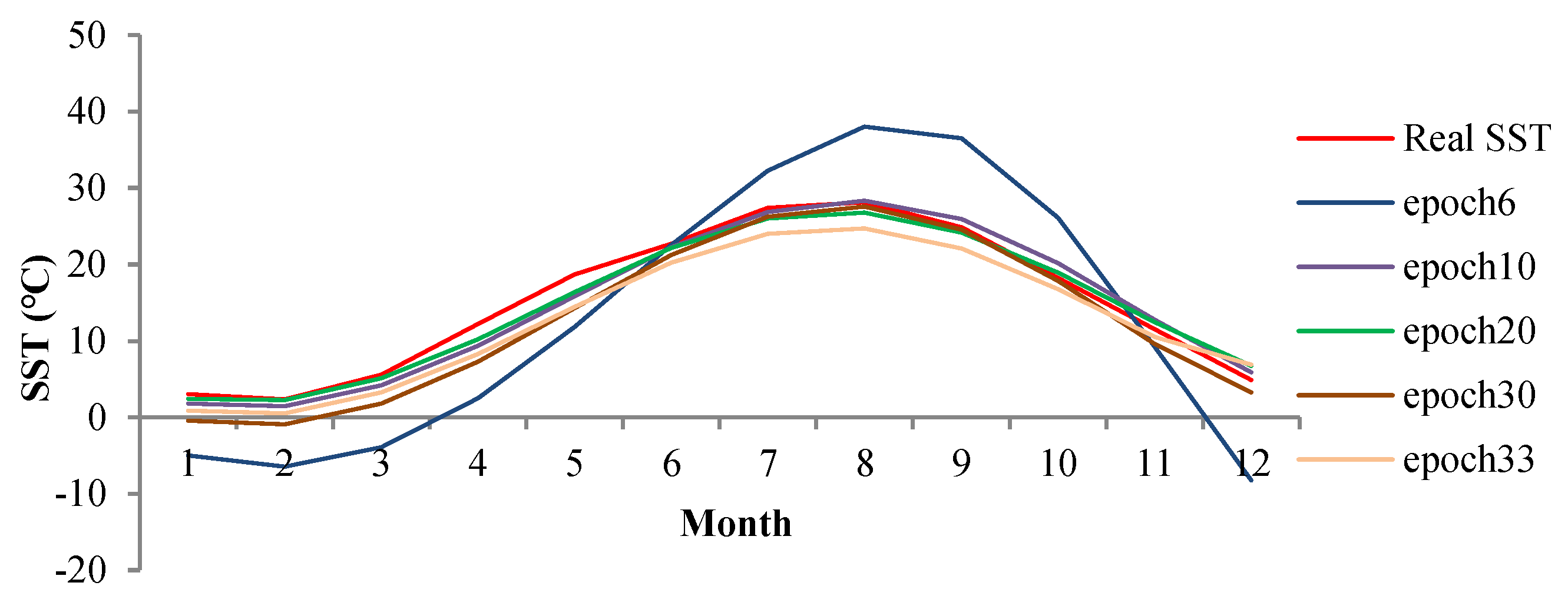
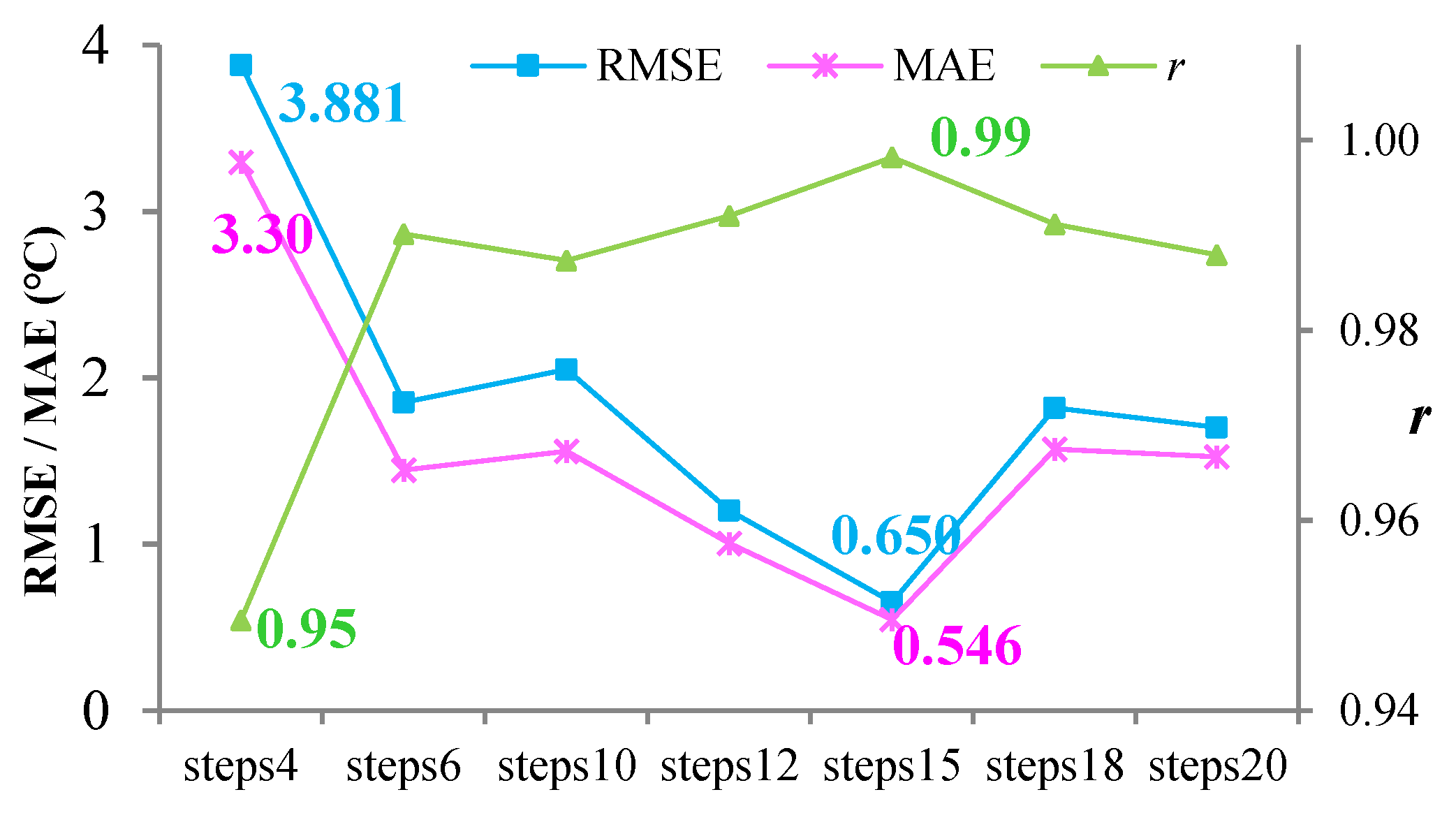
4.2. Results of Using Different Parameters

In the network model, steps_per_epoch (steps) refers to the number of steps contained in an epoch, and each step is a batch of data input; epochs indicate each data traversal time. The proposed model is trained by reading data in time series. When all data are covered, the iteration stops. Therefore, epochs and steps in the network model cannot be simultaneously set to be too large. This study uses the monthly data of a P2 site to predict the SST for the next 12 months (January 2019 to December 2019) and explores the optimal parameters by setting different steps and epochs.

Figure 5 shows the SST prediction results for 12 months under different epochs. The results show that epoch 6 cannot accurately predict the overall trend of SST, whereas the other four epochs can effectively predict the trend of SST. For epoch 6, the prediction performance of August is the worst of the entire year, and an unrealistic SST is predicted for winter months as well. Figure 6 presents the quantitative prediction accuracy. With the increase in epochs, the prediction accuracy of the model initially increases and then tends to stabilize with a slight decrease. For epoch 20, the prediction accuracy is the highest, with an RMSE of 1.273 °C, MAE of 1.077 °C, and r of 0.99.

Figure 7 displays the SST prediction results for 12 months under different steps. The results show that the predictions of the SST variation—except for step 4—are satisfactory and agree with the real SST. Figure 8 exhibits the prediction accuracy under different steps, and the results continue to show that the prediction accuracy initially increases and then decreases with the increase in steps. In this study, step 15 has the highest accuracy with an RMSE of 0.650 °C, MAE of 0.546 °C, and r of 1.00.

4.3. Monthly Data Prediction

The last 4, 6, 12, 18, and 24 months are predicted using the optimal parameters of steps and epochs, which are set as 15 and 20, respectively. The P2 site is used as an example to draw the prediction curves, as shown in Figure 9. The horizontal axis is the predicted monthly SST data. For example, the last 4 months refer to the 4 months from December 2019 to the historical months; i.e., the predicted months are September, October, November, and December 2019.

In terms of the fitting degree, the proposed network model is superior to LSTM except for the prediction length of step 4. With the increase in prediction length, the advantage is gradually evident. Figure 10 illustrates the prediction accuracy of quantitative analysis.

Figure 10 shows that the accuracy of the proposed model and LSTM tends to decline with the increase in prediction time. However, in comparison with LSTM, the SST prediction error based on the proposed model fluctuates and exhibits a more stable accuracy. The r values of the proposed model using different prediction lengths are all above 0.98; in contrast, when using LSTM, r is lower than 0.88 when the prediction runs for 24 months. The accuracy of LSTM prediction is slightly higher than that of the proposed model when the prediction length is 4 months, with an RMSE of 0.325 °C and MAE of 0.251 °C. However, when the prediction length is increased, the accuracy of the SST prediction model based on the proposed model is significantly higher than that of LSTM, especially for 18 and 24 months, and the RMSE is 1.129 °C and MAE is 1.275 °C.

However, as shown in Figure 11, we can see from the quantitative prediction results of each month that the LSTM and the proposed model have a large prediction error in May of each year. The MAEs of the proposed model and LSTM are 2.641 °C and 4.401 °C for the first May (fifth month) and 4.159 °C and 7.030 °C for the second May (17th month), respectively. The possible reason for this is that April to May is the period with the largest temperature change in the entire year, and the prediction model conservatively predicts the SST. In terms of the monthly prediction accuracy of Figure 11, the maximum error occurs in the 17th month, with an MAE of 4.2 °C by the proposed model and 7.0 °C by LSTM.

To test the stability of the SST prediction neural network model based on the proposed model, we conducted a quantitative evaluation of the prediction results of six sites with different time lengths.

Table 2. Monthly RMSE and MAE of six sites with different predicted lengths (the unit is °C).

	Site	Pre_4m 1		Pre_6m 1		Pre_12m 1		Pre_18m 1		Pre_24m 1
		RMSE	MAE	RMSE	MAE	RMSE	MAE	RMSE	MAE	RMSE	MAE
LSTM	P1	0.631	0.567	1.345	1.176	1.603	1.373	1.386	1.108	2.881	2.238
	P2	0.324	0.263	1.670	1.512	2.189	1.908	2.097	4.389	9.954	3.440
	P3	1.000	0.937	1.742	1.582	1.772	1.486	1.973	1.736	3.785	2.644
	P4	0.616	0.545	1.423	1.183	4.248	3.288	1.958	1.750	1.986	1.494
	P5	0.517	0.457	2.298	1.929	1.899	1.565	1.496	1.247	1.775	1.402
	P6	0.231	0.200	1.711	1.384	1.466	1.246	2.645	2.060	1.328	0.986
Proposed model	P1	1.362	1.286	0.598	0.552	1.247	1.168	1.112	1.026	1.613	1.275
	P2	0.653	0.569	0.717	0.570	1.258	1.027	1.129	1.275	3.196	1.124
	P3	0.677	0.539	1.370	1.261	1.128	0.933	1.645	1.461	2.891	2.353
	P4	1.205	1.160	1.216	1.061	1.293	1.153	1.271	1.018	1.419	1.083
	P5	0.862	0.807	1.089	0.908	1.256	1.044	1.355	1.158	1.636	1.286
	P6	1.155	1.106	1.159	1.477	0.929	0.810	1.676	1.294	1.167	0.991

¹ Pre_4m, Pre_6m, Pre_12m, Pre_18m, Pre_24m refer to the prediction lengths of 4, 6, 12, 18, and 24 months for monthly data, respectively.

presents the results.

A comparison of the prediction results of the six sites indicates that, except for P3, LSTM has a slight advantage over the proposed model in predicting the SST in a short time; for example, in the 4 month prediction. The maximum differences of RMSE and MAE between LSTM and the proposed model occurred at P6, at 0.924 °C and 0.906 °C, respectively. On the whole, in the short prediction length (4 month prediction), the mean differences of RMSE and MAE between LSTM and the proposed model are 0.540 °C and 0.549 °C, respectively, and LSTM is better than the proposed method in terms of prediction performance. However, with an increased prediction time, the SST prediction results of the proposed model are significantly better than those of LSTM. The mean differences of RMSE and MAE between the proposed model and LSTM are 1.292 °C and 0.701 °C, respectively, and the proposed method is better than LSTM in terms of prediction performance. Moreover, the monthly SST data prediction based on the proposed method is more robust and accurate.

4.4. Quarterly Data Prediction

A total of 152 items of quarterly data are used in every site. Different time lengths, such as the last 2, 4, 6, and 8 quarters, are predicted on the basis of the model trained by quarterly data. P2 site data are used as an example to draw the prediction curves, as shown in Figure 12.

From the perspective of fitting degree, although the proposed model and LSTM can effectively predict the trend of SST, the SST prediction model based on the proposed model is superior to the LSTM regardless of the prediction length. When the prediction length is small, such as over two quarters, the difference of prediction accuracy between the two models is small, at about 0.3 °C. Overall, the SST prediction error of quarterly data is within 2 °C based on the proposed method; however, the prediction error based on LSTM can reach 3.5 °C. With the increase of prediction length, the GRU model is relatively stable, while LSTM fluctuates greatly, especially when the prediction length is 4. By comparing the curves under the four prediction lengths, the prediction results of the two prediction models are slightly lower than the true SST value. Thus, both models have the characteristics of conservative prediction. Figure 13 presents the prediction accuracy of the P2 site’s quarterly data.

As shown in Figure 13, with the increase in prediction time, the error based on the proposed prediction model does not present a significant increasing trend. The proposed model exhibits a further stable performance with high prediction accuracy. The RMSE and MAE are both within 2 °C, and r is above 0.98.

Table 3. Quarterly RMSE and MAE of six sites with different predicted lengths (the unit is °C).

	Location	Pre_2q 1		Pre_4q 1		Pre_6q 1		Pre_8q 1
		RMSE	MAE	RMSE	MAE	RMSE	MAE	RMSE	MAE
LSTM	P1	1.676	1.636	2.150	2.023	2.810	3.045	3.482	3.336
	P2	1.964	1.842	3.907	3.513	2.276	2.315	2.980	2.865
	P3	3.006	2.334	2.829	2.039	2.175	2.042	3.426	2.711
	P4	2.698	2.683	2.292	1.975	1.245	0.993	1.748	1.496
	P5	1.578	1.325	2.751	2.433	0.727	0.699	1.395	1.025
	P6	1.856	1.587	2.214	1.882	1.593	1.737	2.415	2.264
Proposed model	P1	1.593	1.575	2.153	1.848	1.86	1.976	1.577	1.305
	P2	1.636	1.636	1.628	1.545	1.536	1.553	1.948	1.743
	P3	2.239	1.955	0.993	0.794	1.692	1.679	3.423	2.896
	P4	2.302	2.165	1.673	1.267	0.937	0.909	0.892	0.687
	P5	1.326	1.012	2.635	2.393	0.714	0.705	1.049	0.883
	P6	1.504	1.153	1.870	1.763	1.135	1.126	1.600	1.275

¹ Pre_2q, Pre_4q, Pre_6q, Pre_8q refer to the prediction length of 2, 4, 6, and 8 for quarterly data, respectively.

displays the quantitative results of prediction accuracy for different quarterly lengths for the six sites. In contrast to the monthly data, quarterly SST prediction results based on the proposed model indicate better prediction accuracy than those based on LSTM, even with a short-term prediction length. The maximum differences of RMSE and MAE between LSTM and proposed model occurred at P2, at 1.095 °C and 1.015 °C, respectively. The minimum is P5, and the differences of RMSE and MAE are 0.182 °C and 0.122 °C, respectively. The mean MAEs of the six sites for a predicting length of 2, 4, 6, and 8 quarters based on the proposed method are 1.422 °C, 1.675°C, 1.246°C, and 1.536 °C respectively. For LSTM, these values are 1.801 °C, 1.924 °C, 1.537 °C, and 1.843 °C, respectively. Moreover, the quarterly SST data prediction based on the proposed method is more robust and accurate.

5. Conclusions

In this study, a neural network model based on GRU with fully connected layers is designed to predict short and medium-term SST. By using the Bohai Sea, characterized by a large annual temperature difference, as the research area, two different time scales of monthly and quarterly SST data are used to verify the practicability and stability of the proposed model. The main conclusions are as follows:

(1)

The designed SST prediction model based on GRU can efficiently fit the trend of the real SST and has high reliability. Additionally, the proposed model in this paper has the characteristics of a conservative estimation for SST prediction; that is, the predicted value of SST is smaller than the real value. Furthermore, LSTM experiences the same problem as the proposed method in this paper.

(2)

In the prediction at the monthly time scale, RMSE and MAE are mostly concentrated in the range of 0–2.5 °C. In the prediction at the quarterly time scale, RMSE and MAE are mostly concentrated in the range of 0–2 °C. The r values of both time scales are above 0.98, indicating high prediction accuracy.

(3)

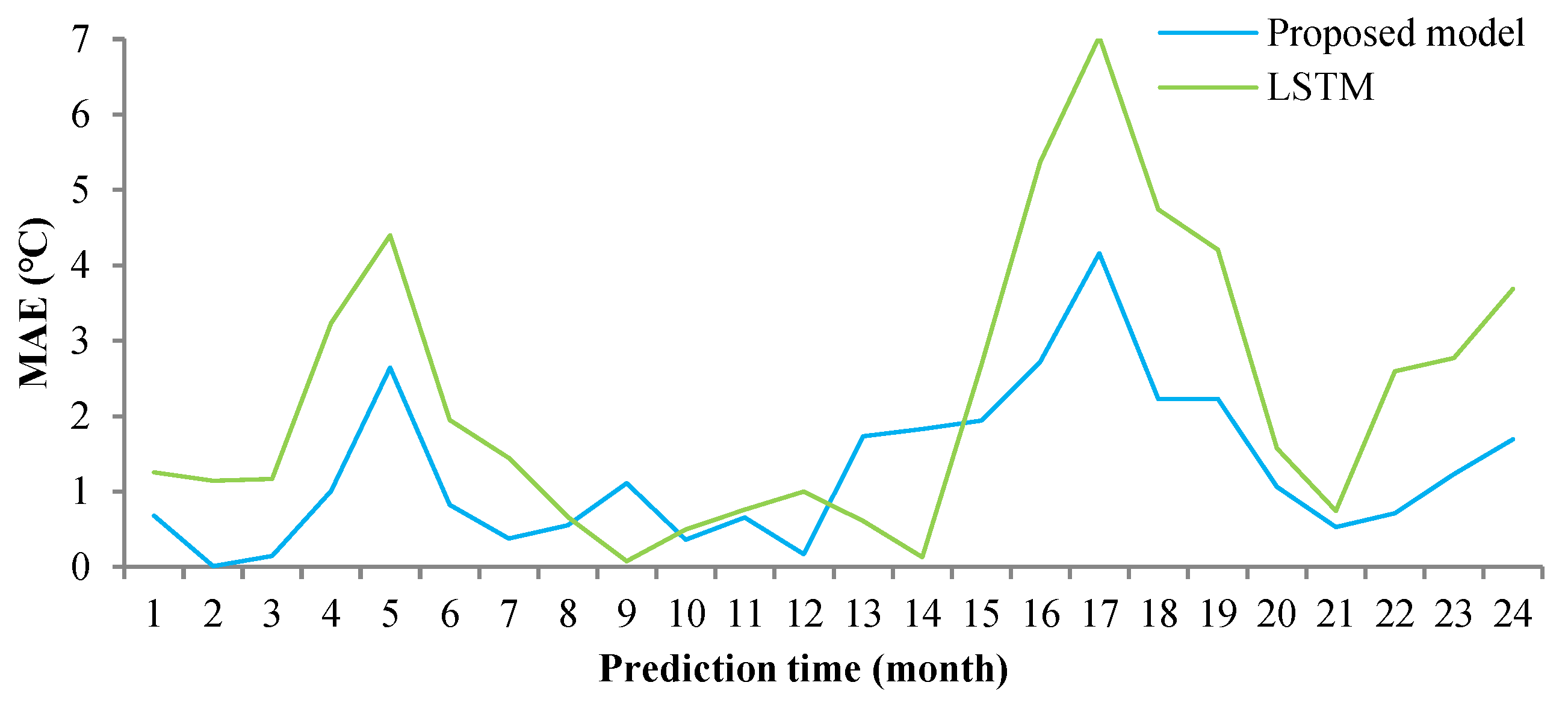
The proposed prediction model has more stable results than LSTM. The advantages are more evident with an increase in prediction length.

In future, the multi-source physical ocean parameters of the GRU network can be investigated to construct a physical prediction model of SST. Besides, there may be local outliers on a smaller spatial scale, so the GRU SST prediction method considering the spatial relationship may effectively improve the fault tolerance and prediction accuracy of SST.

References

1. Frank, J.; Wentz, C.G.; Smith, D.; Chelton, D. Satellite measurements of sea surface temperature through clouds. Science 2000, 288, 847–850. [Google Scholar] [CrossRef] [Green Version]
2. Sumner, M.D.; Michael, K.J.; Bradshaw, C.J.; Hindell, M.A. Remote sensing of Southern Ocean sea surface temperature: Implications for marine biophysical models. Remote Sens. Environ. 2003, 84, 161–173. [Google Scholar] [CrossRef]
3. Sun, W.; Zhang, J.; Meng, J.; Liu, Y. Sea surface temperature characteristics and trends in China offshore seas from 1982 to 2017. J. Coast. Res. 2019, 90, 27–34. [Google Scholar] [CrossRef]
4. Bouali, M.; Sato, O.T.; Polito, P.S. Temporal trends in sea surface temperature gradients in the South Atlantic Ocean. Remote Sens. Environ. 2017, 194, 100–114. [Google Scholar] [CrossRef]
5. Herbert, T.D.; Peterson, L.C.; Lawrence, K.T.; Liu, Z. Tropical Ocean Temperatures over the Past 3.5 Million Years. Science 2010, 328, 1530–1534. [Google Scholar] [CrossRef] [PubMed]
6. Yao, S.-L.; Luo, J.-J.; Huang, G.; Wang, P. Distinct global warming rates tied to multiple ocean surface temperature changes. Nat. Clim. Chang. 2017, 7, 486–491. [Google Scholar] [CrossRef]
7. Solanki, H.U.; Bhatpuria, D.; Chauhan, P. Signature analysis of satellite derived SSHa, SST and chlorophyll concentration and their linkage with marine fishery resources. J. Mar. Syst. 2015, 150, 12–21. [Google Scholar] [CrossRef]
8. Kim, D.-I. Effects of temperature, salinity and irradiance on the growth of the harmful red tide dinoflagellate Cochlodinium polykrikoides Margalef (Dinophyceae). J. Plankton Res. 2004, 26, 61–66. [Google Scholar] [CrossRef]
9. Li, S.; Goddard, L.; Dewitt, D.G. Predictive Skill of AGCM Seasonal Climate Forecasts Subject to Different SST Prediction Methodologies. J. Clim. 2008, 21, 2169–2186. [Google Scholar] [CrossRef]
10. Patil, K.; Deo, M.C.; Ravichandran, M. Prediction of Sea Surface Temperature by Combining Numerical and Neural Techniques. J. Atmos. Ocean. Technol. 2016, 33, 1715–1726. [Google Scholar] [CrossRef]
11. Krishnamurti, T.N.; Chakraborty, A.; Krishnamurti, R.; Dewar, W.K.; Clayson, C.A. Seasonal Prediction of Sea Surface Temperature Anomalies Using a Suite of 13 Coupled Atmosphere–Ocean Models. J. Clim. 2006, 19, 6069–6088. [Google Scholar] [CrossRef]
12. Stockdale, T.N.; Balmaseda, M.A.; Vidard, A. Tropical Atlantic SST prediction with coupled ocean–atmosphere GCMs. J. Clim. 2006, 19, 6047–6061. [Google Scholar] [CrossRef]
13. Laepple, T.; Jewson, S. Five Year Ahead Prediction of Sea Surface Temperature in the Tropical Atlantic: A Comparison between IPCC Climate Models and Simple Statistical Methods. arXiv 2007, arXiv:physics/0701165. [Google Scholar]
14. Xue, Y.; Leetmaa, A. Forecasts of tropical Pacific SST and sea level using a Markov model. Geophys. Res. Lett. 2000, 27, 2701–2704. [Google Scholar] [CrossRef] [Green Version]
15. Li, J.K.; Zhao, Y.; Liao, H.L. SST forecast based on BP neural network and improved EMD algorithm. Clim. Environ. Res. 2017, 22, 587–600. [Google Scholar] [CrossRef]
16. Lins, I.D.; Araujo, M.; das Chagas Moura, M.; Silva, M.A.; Droguett, E.L. Prediction of sea surface temperature in the tropical Atlantic by support vector machines. Comput. Stat. Data Anal. 2013, 61, 187–198. [Google Scholar] [CrossRef]
17. Martinez, S.A.; Hsieh, W.W. Forecasts of tropical Pacific sea surface temperatures by neural networks and support vector regression. Int. J. Oceanogr. 2009, 1–13. [Google Scholar] [CrossRef] [Green Version]
18. Álvarez, A.; López, C.; Riera, M.; Hernández-García, E.; Tintoré, J. Forecasting the SST Space-time variability of the Alboran Sea with genetic algorithms. Geophys. Res. Lett. 2000, 27, 2709–2712. [Google Scholar] [CrossRef] [Green Version]
19. Garcia-Gorriz, E.; Garcia-Sanchez, J. Prediction of sea surface temperatures in the western Mediterranean Sea by neural networks using satellite observations. Geophys. Res. Lett. 2007, 34. [Google Scholar] [CrossRef]
20. Patil, K.; Deo, M.C. Prediction of daily sea surface temperature using efficient neural networks. Ocean Dyn. 2017, 67, 357–368. [Google Scholar] [CrossRef]
21. Zhang, Q.; Wang, H.; Dong, J.; Zhong, G.; Sun, X. Prediction of Sea Surface Temperature Using Long Short-Term Memory. IEEE Geosci. Remote Sens. Lett. 2017, 14, 1745–1749. [Google Scholar] [CrossRef] [Green Version]
22. LeCun, Y.; Bengio, Y.; Hinton, G. Deep learning. Nature 2015, 521, 436–444. [Google Scholar] [CrossRef] [PubMed]
23. Yang, Y.; Dong, J.; Sun, X.; Lima, E.; Mu, Q.; Wang, X. A CFCC-LSTM Model for Sea Surface Temperature Prediction. IEEE Geosci. Remote Sens. Lett. 2018, 15, 207–211. [Google Scholar] [CrossRef]
24. Liu, H.; Tian, H.; Li, Y.; Zhang, L. Comparison of four Adaboost algorithm based artificial neural networks in wind speed predictions. Energy Conv. Manag. 2015, 92, 67–81. [Google Scholar] [CrossRef]
25. Xiao, C.; Chen, N.; Hu, C.; Wang, K.; Gong, J.; Chen, Z. Short and mid-term sea surface temperature prediction using time-series satellite data and LSTM-AdaBoost combination approach. Remote Sens. Environ. 2019, 233, 111358. [Google Scholar] [CrossRef]
26. Messias, V.R.; Estrella, J.C.; Ehlers, R.; Santana, M.J.; Santana, R.C.; Reiff-Marganiec, S. Combining time series prediction models using genetic algorithm to autoscaling Web applications hosted in the cloud infrastructure. Neural Comput. Appl. 2015, 27, 2383–2406. [Google Scholar] [CrossRef] [Green Version]
27. Dey, R.; Salemt, F.M. Gate-variants of Gated Recurrent Unit (GRU) neural networks. In Proceedings of the IEEE 60th International Midwest Symposium on Circuits and Systems (MWSCAS), Boston, MA, USA , 6–9 August 2017; pp. 1597–1600. [Google Scholar] [CrossRef] [Green Version]
28. Rana, Rajib. Gated Recurrent Unit (GRU) for Emotion Classification from Noisy Speech. arXiv 2016, arXiv:1612.07778.
29. Agarap, A.F.M. A Neural Network Architecture Combining Gated Recurrent Unit (GRU) and Support Vector Machine (SVM) for Intrusion Detection in Network Traffic Data. In Proceedings of the 2018 10th International Conference on Machine Learning and Computing-ICMLC 2018, Macau, China, 26–28 February 2018; 2018; pp. 26–30. [Google Scholar] [CrossRef] [Green Version]
30. Wang, F.; Shi, X.; Su, J. A Sentence Segmentation Method for Ancient Chinese Texts Based on Recurrent Neural Network. Acta Sci. Nat. Univ. Pekin. 2017, 53, 255–261. [Google Scholar] [CrossRef]
Figure 1. Study area in the Bohai Sea. The six selected sites are as follows: P1 (118.625° E, 38.375° N), P2 (119.125° E, 38.875° N), P3 (119.625° E, 37.375° N), P4 (119.625° E, 39.375° N), P5 (120.125° E, 38.375° N), and P6 (120.625° E, 39.375° N).
Jmse 08 00249 g001
Figure 2. Structure diagram of long short-term memory (LSTM) and gated recurrent unit (GRU) methods. The upper part is LSTM [25] and the lower part is GRU [27]. Jmse 08 00249 i001 indicates the sigmoid and tanh neural network layers. Jmse 08 00249 i002 represents the pointwise multiplication and addition operations. Jmse 08 00249 i003 is the operation subtracted by 1. Jmse 08 00249 i004 depicts the input time series data. Jmse 08 00249 i005 exhibits the output data.
Jmse 08 00249 g002
Figure 3. Model structure used in this study for medium and long-term SST prediction.
Jmse 08 00249 g003
Figure 4. Monthly and quarterly data used in this paper. (a) Monthly data used in this paper. (b) Quarterly data used in this paper.
Jmse 08 00249 g004
Figure 5. SST prediction for 12 months under different epochs.
Jmse 08 00249 g005
Figure 6. Prediction accuracy for 12 months under different epochs. RMSE: root mean square error; MAE: mean absolute error.
Jmse 08 00249 g006
Figure 7. SST prediction for 12 months under different steps.
Jmse 08 00249 g007
Figure 8. Prediction accuracy for 12 months under different steps.
Jmse 08 00249 g008
Figure 9. P2 prediction results for different time lengths. The horizontal axis is the predicted length (month). (a) Prediction for the last 4 months; (b) Prediction for the last 6 months; (c) Prediction for the last 12 months; (d) Prediction for the last 18 months; (e) Prediction for the last 24 months.
Jmse 08 00249 g009
Figure 10. Prediction accuracy for different monthly lengths of the P2 site. (a) RMSE with different prediction length; (b) MAE with different prediction length; (c) r with different prediction length.
Jmse 08 00249 g010
Figure 11. Twenty-four-month prediction accuracy.
Jmse 08 00249 g011
Figure 12. Prediction results under different quarterly lengths for the P2 site. (a) Prediction for the last 2 quarters; (b) Prediction for the last 4 quarters; (c) Prediction for the last 6 quarters; (d) Prediction for the last 8 quarters.
Jmse 08 00249 g012
Figure 13. Prediction accuracy for different time lengths for the P2 site. (a) RMSE with different prediction lengths; (b) MAE with different prediction lengths; (c) r with different prediction lengths.
Jmse 08 00249 g013