An Overview of the Expected Shoreline Impact of the Marine Energy Farms Operating in Different Coastal Environments

Abstract

The aim of the present work is to provide an overview of the possible implications involving the influence of a generic marine energy farm on the nearshore processes. Several case studies covering various European coastal areas are considered for illustration purposes. These include different nearshore areas, such as the Portuguese coast, Sardinia Island or a coastal sector close to the Danube Delta in the Black Sea. For the case studies related to the Portuguese coast, it is noted that a marine energy farm may reduce the velocity of the longshore currents, with a complete attenuation of the current velocity for some case studies in the coastal area from Leixoes region being observed. For the area located close to the Danube Delta, it is estimated that in the proposed configuration, a marine energy farm would provide an efficient protection against the wave action, but it will have a relatively negligible impact on the longshore currents. Summarizing the results, we can conclude that a marine energy farm seems to be beneficial for coastal protection, even in the case of the enclosed areas, such as the Mediterranean or Black seas, where the erosion generated by the wave action represents a real problem.

1. Introduction

A significant part of the global population lives near the coastal areas. It is estimated that almost 20% of the total population is located in a strip area of 25 km from the coast. The share increases to up to 40% of the total population when extending the considered strip area to 100 km. A particularity of these areas is that they are very dynamic environments, which present an annual urban growth of 2.6%. At the same time, the number of coastal cities has itself increased about 4.5 times since 1950 [1,2]. Although these areas are defined by numerous opportunities, they are also facing some threats coming from the surrounding environment, such as coastal erosion, a natural event during which the balance between accretion and erosion is continuously shifting [3,4,5,6]. These natural events occur on various spatial and temporal scales, being influenced by many factors, such as wind, waves and nearshore currents. Moreover, it is expected that climate change will have a negative impact on coastal areas in the future, with sea levels being supposed to rise and the marine conditions becoming more aggressive [7,8,9].

Although multiple parameters shape the coastline processes, the wave action has a significant impact on the coastal erosion [10,11,12]. This aspect was highlighted by Bacino et al. [13], when assessing a beach sector (Samborombón Bay) near the Argentinean coast. In this case, a direct correlation was established between the higher levels of the wave energy and the severe erosion. The wave run-up erosion was studied by Feagin et al. [14], who concluded that dune vegetation will significantly reduce the coastal erosion caused by the storm events. In the work of Serafim et al. [15], the importance of considering the wave action in the set-up of a coastal management plan was highlighted through a case study focused on the Santa Catarina region (southern Brazil). An extreme event is expected to have a negative impact on the beach stability, as in the case of the storm Xynthia that hit the French Atlantic coast in February 2010 [16]. During this event, most of the coastal dunes were affected by breaches, with a strong shoreline retreat being noticed for Saint-Hilaire-de-Riez (−5 m) and La Tranche-sur-Mer (−15 m). The correlation between the storm intensity and coastal erosion was also addressed in Montreuil et al. [17], where an erosion index was established.

At present, most of the erosion management strategies involve the use of hard solutions, such as seawalls, interlocking blocks, rubble mound, detached breakwaters, groins, dunes, tyres or jetties [18,19,20,21]. Nevertheless, there are studies indicating that this approach is not the best way to tackle coastal erosion. In this sense, either soft solutions on a standalone basis or an optimal combination of the soft and hard solutions are expected to provide better results. This aspect was highlighted by Liu et al. [22] when investigating China’s coastal engineering system, as well as by Pranzini [23] when focusing on the Italian costal area and by Williams et al. [24] who provided a general overview of this topic.

As the industry evolves, some new technological solutions emerge, such as renewable systems, with wave energy converters (WECs) [25,26,27,28,29] being a prime example. Since the purpose of a WEC farm is to extract energy from the waves, the use of such projects for coastal protection was developed in recent years. Taking into account that at this moment there are no operational wave farms, most of the studies have been based on numerical simulations in which various “what-if’’ scenarios have been considered. This is the case of Bento et al. [30], Rusu and Onea [31] or Zanopol et al. [32], who considered for assessment the effects induced by a wave farm on different coastal environments. A common way to implement a wave farm is by using a line (or an area), defined as a single obstacle which is characterized by various absorption coefficients. This approach is commonly used for the Portuguese environment [33,34]. Furthermore, it is possible to simulate a wave farm that incorporates multiple WECs, this method being used in Diaconu and Rusu [35] or Rusu and Guedes Soares [36].

A full understanding of a wave farm’s impact can be done by considering various transmission coefficients, that can go from 0% (compact farm) up to 90% (widely spaced WECs). This particular aspect was considered in Millar et al. [37] and in Zanopol et al. [38]. A more sophisticated approach involves the combination of a wave propagation model and a coastal circulation model in order to highlight the impact of a wave project on the beach stability. Following this approach, there are numerous studies indicating that the implementation of a marine energy farm is a viable solution for coastal protection [39,40,41]. Driven by the fact that the offshore wind sector is already a mature market, some other works are focused on the analysis of dual wind-wave farms considering various point of views. For example, in Astariz and Iglesias [42,43], the possibility to reduce the downtime period was evaluated by taking into account some specific wind projects, such as Alpha Ventus and Horns Rev I. Various wave farm configurations were also proposed in order to improve the accessibility for operation tasks. Since the wave energy sector is moving forward, the next step is to assemble various wave farms and test their operation. Therefore, it is important to predict in advance the expected coastal impact of such a project [44,45,46,47].

By looking at similar works, we can notice that most of the discussions have been focused on the nearshore impact related to the changes induced in the local wave conditions and little attention has been given to the coastal hydrodynamics and sediment transport processes. As a consequence, the present work aims to cover this gap by providing some insights regarding the littoral drift budget that may be encountered in the presence of a marine energy farm. From the knowledge of the authors, another element of novelty is that for the first time this work considers a generic marine energy farm defined by the same characteristics (length and distance to the shoreline) that are assumed to be implemented in different coastal environments (two located in the ocean and two in enclosed seas). Therefore, the objectives are:

(a) to establish the spatial distribution of the significant wave heights in the presence of a generic wave farm. In addition to this, the shoreline variation of various wave parameters will be considered for investigation;

(b) to identify the distribution of the longshore currents (especially as regards the maximum velocity);

(c) to determine the implications for the coastal hydrodynamics by evaluating the connection between the significant wave heights, the longshore current velocities and the sediment transport.

2. Materials and Methods

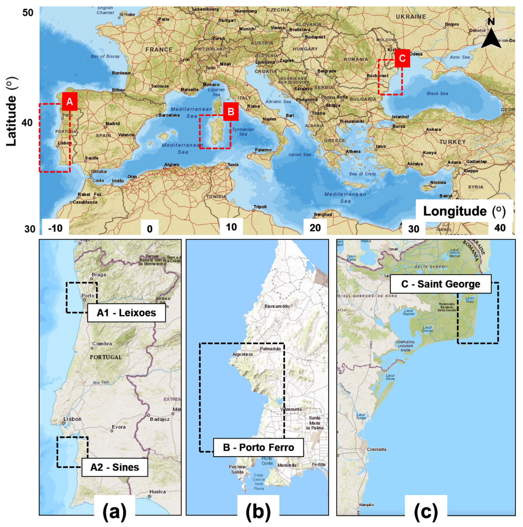
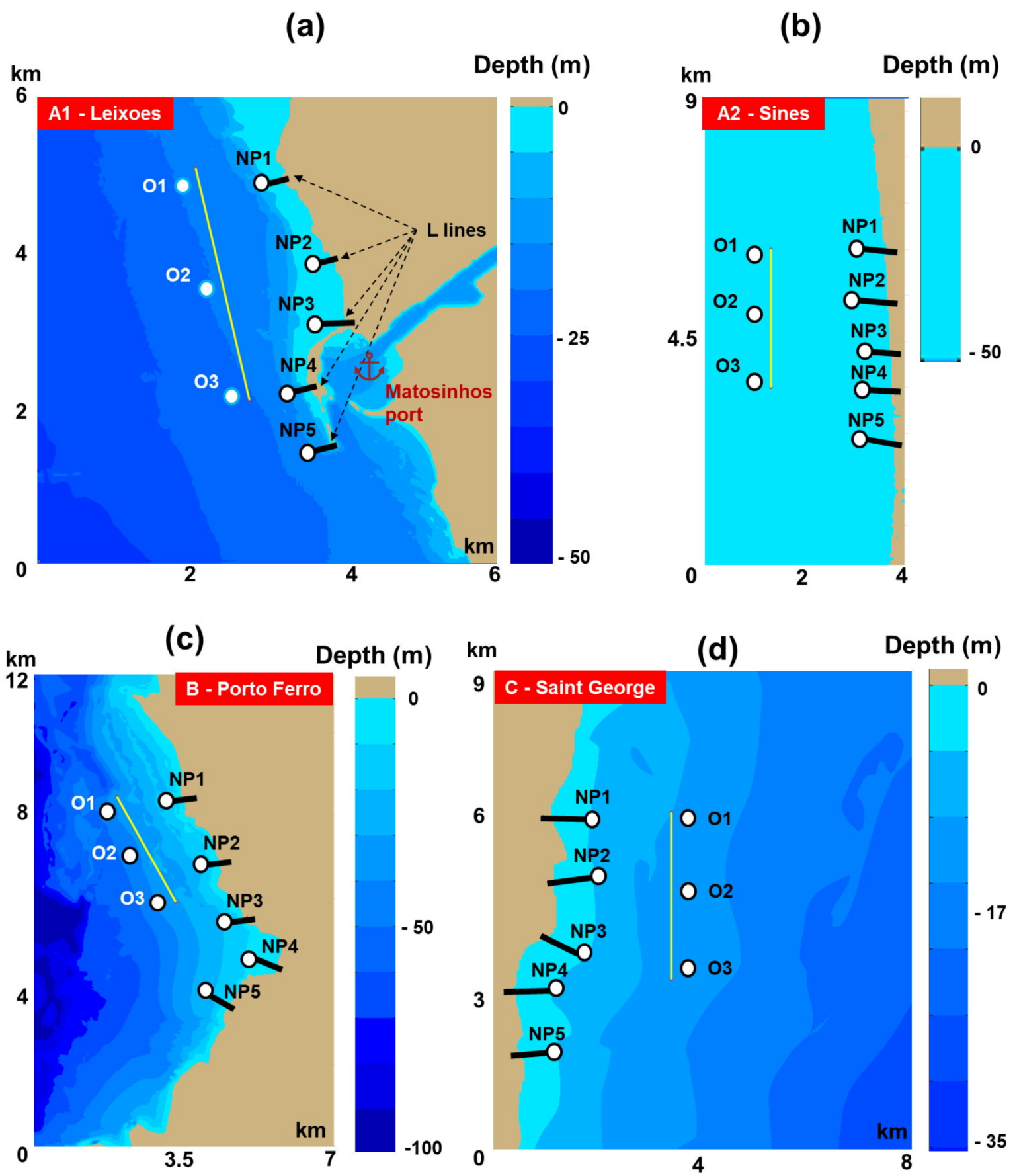
2.1. Target Areas

Four different European coastal areas were considered in this work, two at the North Atlantic Ocean and other two in sea environments (Mediterranean and Black Sea, respectively). These four target areas are illustrated in Figure 1. The first two are related to the nearshore areas facing the ocean environment, more precisely on the Portuguese continental coast (zone A).

In the south of this zone, a coastal sector located close to the Sines peninsula was evaluated, while, in the north, a sector located close to the Leixoes area (north of the city of Porto) was considered. Going east, we identified a second target area (zone B) that is located in the Mediterranean Sea. In this case we evaluated an island environment, Sardinia. The north-western part of the Black Sea was also taken into account (zone C), more precisely the Saint George sector (in the Romanian nearshore), which is part of the Danube Delta.

A first step in the evaluation of the coastal impact is related to the identification of some relevant environmental conditions. In this case, such conditions would be the most important wave parameters, namely: significant wave height—Hs (in meters); mean wave period—Tm (in seconds); mean wave direction—Dir (in degree).

Table 1. Wave conditions defined for the different coastal areas targeted and their characteristics according to various sources [31,32,33,34,38,48].

Area	Conditions	Hs (m)	Tm (s)	Dir (°)
A1—Leixoes (North Atlantic)	Total time average (denoted with total average) Winter time average (winter average) High non-storm (non-storm) Regular storm (storm)	1.5 3 4.5 6	7 8 9 11	300 (corresponding to 30 ° in relation to the normal to the shoreline)
A2—Sines (North Atlantic)	Total average Winter average Non-storm Storm	1.5 3 4.5 6	7 8 9 11	300 (corresponding to 30 ° in relation to the normal to the shoreline)
B—Porto Ferro (Mediterranean Sea)	Winter average Non-storm Storm High storm (denoted with high-storm)	1.5 3 4.5 6	5 6 7 9	300 (corresponding to 30 ° in relation to the normal to the shoreline)
C—Saint George(Black Sea)	Winter average Non-storm Storm High-storm	1.5 3 4.5 6	5 6 7 9	60 (corresponding to 30 ° in relation to the normal to the shoreline)

summarizes the wave statistics. The main idea was to consider approximately the same wave conditions, which are identified as most relevant, in all areas in order to assess and compare the coastal response to the presence of the marine energy farms. From this perspective, it must be highlighted that, although all the four different wave conditions defined are realistic for all the coastal environments considered, they represent in general different categories for the ocean waves than for the sea waves. For example, what represents total time average for the ocean waves is very close to the winter time average in the case of the sea waves and the conditions corresponding to a regular storm in the European side of the North Atlantic is close to a high storm in the nearshores considered for the Mediterranean and Black seas. This assumption was based on various analyses that were performed on the general characteristics of the wave climates in the areas targeted. See, for example, the results presented in [31,32,33,34,38,48].

2.2. The ISSM Model System and the Case Studies Considered

The case studies presented in this work were processed by using the ISSM (Interface for SWAN and Surf Models) modelling tool that combines a wave model with a surf model [49,50,51]. As a first step, the SWAN spectral wave model was used to assess the wave transformation in the coastal areas. This model solves the wave action balance equation that describes the variation of the wave spectrum in geographical, time and spectral spaces. This equation can be summarized as [52]:

$$\frac{\partial N}{\partial t}+\nabla [({\overrightarrow{c}}_g+\overrightarrow{U})N]+\frac{\partial }{\partial \sigma }{c}_{\sigma }N+\frac{\partial }{\partial \theta }{c}_{\theta }N=\frac{S}{\sigma }$$

(1)

where N represents the action density spectrum, $\sigma$ is the relative frequency, $\theta$ is the wave direction, and $\overrightarrow{U}\hspace{0.17em}$ is the velocity of the ambient current (assumed to be uniform). The propagation velocities of the wave energy are the group velocity ${\overrightarrow{c}}_g$ in physical space $\left({\overrightarrow{c}}_g=\partial \sigma /\partial \overrightarrow{k}\right)$, $\hspace{0.17em}{c}_{\sigma }=\dot{\sigma }\hspace{0.17em}$ and $c_{\theta }=\overline{\theta }\hspace{0.17em}$ in spectral space. S represents the sink and source terms.

A more detailed assessment of the nearshore processes (including the longshore currents) was provided by the Navy Standard Surf Model (denoted as Surf) [50], that uses as input in the present case the results coming from the SWAN model, more precisely the parameters Hs, Tm and Dir. Tm and Dir are used as direct inputs, while for the wave height it is required to use the root mean square wave height (Hrms) and therefore this parameter is deduced from the significant wave height with the relationship Hrms = 0.707Hs. As for the longshore currents variations, the Surf model uses the following expression [53]:

$${\tau }_y^r+\rho \frac{\partial }{\partial x}\left[\mu h\frac{\partial V}{\partial x}\right]-\langle {\tau }_y^b\rangle +\langle {\tau }_y^w\rangle =0$$

(2)

where ${\tau }_y^r$ represents the longshore directed radiation stress (induced by the incident waves), the second term is the horizontal mixing due to cross-shore gradients in the longshore current velocity V, ${\tau }_y^b$ is the wave averaged bottom stress, and ${\tau }_y^w$ is the long-shore wind stress. At this point, it is important to mention that this modelling system was implemented and validated for all the target areas considered for evaluation [54,55,56]. Some additional details regarding the main characteristics and physical processes are presented in

Table 2. Characteristics of the SWAN simulations corresponding to the computational domains defined for the target areas considered.

Input/ Process	Wave	Wind	Tide	Crt	Gen	Wcap	Quad	Triad	Diff	Bfric	Setup	Br
	x	x	-	x	x	x	x	x	x	x	x	x
Model SWAN	Coordinates	∆x × ∆y (m)		∆θ (°)		Mod		nf	nθ	ngx × ngy = np
Leixoes	Cartesian	25 × 25		5		Stat/BSBT		34	36	233 × 236 = 54,988
Sines	Cartesian	50 × 50		5		Stat/BSBT		34	36	218 × 502 = 109,436
Porto Ferro	Cartesian	25 × 25		5		Stat/BSBT		34	36	288 × 459 = 132,192
Saint George	Cartesian	50 × 50		5		Stat/BSBT		36	34	354 × 405 = 143,370

. In this table, $\Delta x$ and $\Delta y$ are the resolutions in the geographical space,$\Delta \theta$ is the resolution in the directional space, $nf$ is the number of frequencies in the spectral space, $n\theta$ is the number of directions in the spectral space, $ngx$ and $ngy$ are the number of grid points in x and y direction, and $np$ is the total number of grid points. The input fields considered in the computational domain are: wave forcing (wave), tide forcing (tide), wind forcing (wind) and currents fields (crt). The physical processes activated are: generation by wind (gen), whitecapping process (wcap), quadruplet nonlinear interactions (quad), triad nonlinear interactions (triad), diffraction process (dif), bottom friction (bfric), wave-induced setup (setup) and activation of the depth-induced wave breaking (br).

Figure 2 illustrates the case studies considered. For each target area, a line of 3 km in length was considered, aiming to replicate the influence of a generic marine energy farm. A 2 km distance between the marine energy farm and the shoreline was considered, while the orientation of the farm was made according to the particularity of each target area.

The variations of the wave conditions in the presence of the marine energy farm will be assessed in the geographical space through spatial maps, while a deeper analysis of these fluctuations will be highlighted along the L—reference lines, or by the analysis performed in some offshore and nearshore points (O—points or NP—points).

In order to provide a complete picture of the influence of an energy farm, two case studies were evaluated, as can be noticed from

Table 3. Set-up of the generic wave farm.

Case Study	Transmission (0%—No Farm; 100%—Complete Blockage)	Reflection (0%—No Farm; 100%—Complete Reflection)
Moderate absorption (M-farm)	20%	5%
High absorption (H-farm)	40%	10%

. The first one involved a realistic scenario where the wave farm was defined by a moderate absorption (denoted with M-farm) considering an absorption percentage of only 20% of the incoming waves. The other case study was related to a high absorption scenario (denoted with H-farm) and involved absorption of almost 40% of the waves, this being the case of a wave farm defined by several lines of WECs.

3. Results

3.1. Assessment of the Wave Characteristics

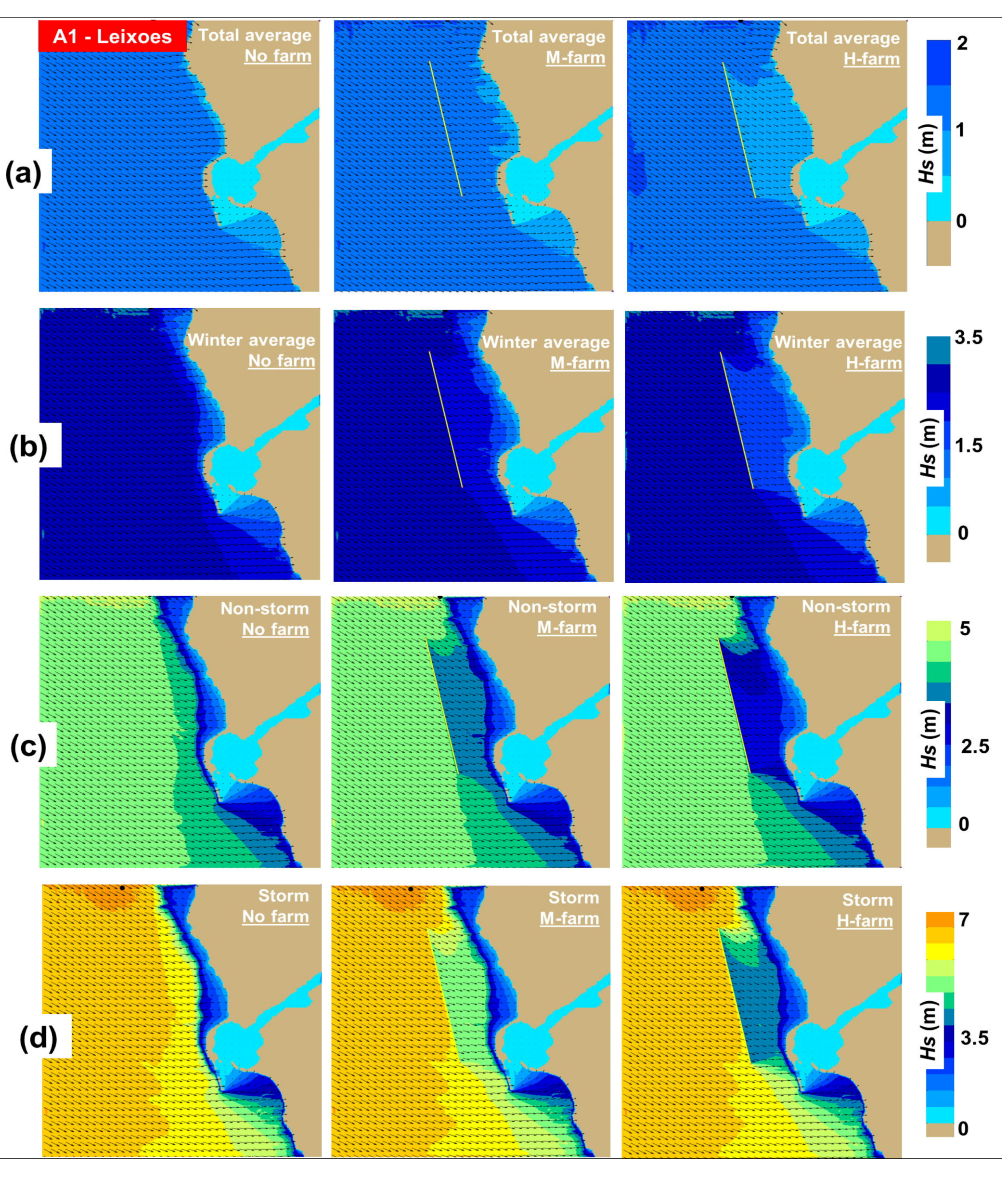
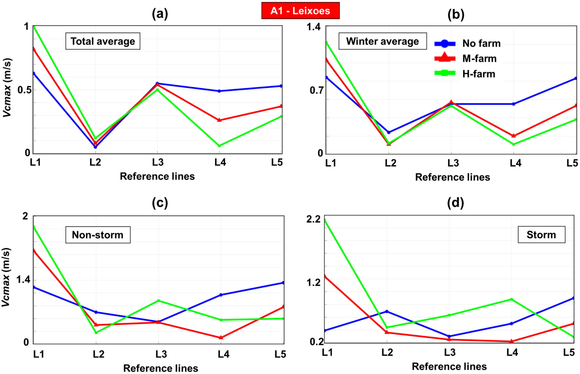
3.1.1. Leixoes (North Atlantic)

The spatial variations of the waves in the Leixoes sector are presented in Figure 3, considering only the waves coming from the north-western sector. As we go from the no farm situation to the high absorption scenario, it is clear that the impact of the wave farm is more visible, especially in the case of a storm, where multiple wave fields are noticed.

The offshore points from this area present the following Hs values, that can range from ~1.4 m (total average) to almost 5.62 m (storm conditions). For the total time period, the waves behind the marine energy farm may be reduced to a minimum of 0.5 m, while the harbour area appears not to be influenced by the presence of the farm. Regarding higher energy case studies, it is possible to notice that the direction of the waves represents an important factor for the coastal areas, the shielding effect of the farm being more visible in the lower part of this region.

Table 4. Leixoes case study—variation of the wave parameters in the presence of the marine energy farm corresponding to the five nearshore points. The results are indicated for all the case studies considered, where: (a) Hs (significant wave height); (b) wave force; c) Vbot (orbital velocity at the bottom) values.

Scenario	(a) Hs values (m)
	Total average					Winter average
No farm	1.25	1.09	1.18	1.26	1.27	2.34	1.40	1.65	2.46	2.45
M-farm	1.12	0.95	0.96	1.03	1.20	2.16	1.34	1.55	2.03	2.33
H-farm	1.01	0.79	0.76	0.86	1.17	1.97	1.25	1.39	1.68	2.27
	Non-storm					Storm
No farm	3.10	1.53	1.85	3.66	3.62	3.70	1.66	2.01	4.94	4.89
M-farm	2.88	1.48	1.78	3.05	3.46	3.50	1.62	1.97	4.21	4.71
H-farm	2.68	1.42	1.66	2.55	3.38	3.26	1.56	1.88	3.56	4.62
	(b) Force values (N/m2)
	Total average					Winter average
No farm	6.16	1.05	0.93	1.15	0.52	10.40	5.00	4.26	4.19	2.35
M-farm	4.99	0.51	0.74	0.78	0.45	12.40	3.65	2.74	3.07	2.05
H-farm	4.07	0.41	0.45	0.53	0.42	13.20	2.98	0.88	2.59	1.88
	Non-storm					Storm
No farm	26.80	8.02	7.69	8.19	5.73	76.60	9.93	10.90	7.60	11.80
M-farm	16.10	6.84	6.01	6.65	4.98	54.80	9.35	9.62	11.10	10.40
H-farm	11.30	5.09	4.11	5.58	4.57	38.20	7.97	7.36	10.40	9.63
	(c) Vbot values (m/s)
	Total average					Winter average
No farm	0.73	0.94	0.89	0.32	0.24	1.50	1.20	1.30	0.73	0.57
M-farm	0.66	0.80	0.71	0.26	0.23	1.40	1.20	1.20	0.60	0.54
H-farm	0.59	0.66	0.56	0.21	0.22	1.20	1.10	1.10	0.50	0.53
	Non-storm					Storm
No farm	2.00	1.30	1.50	1.20	0.95	2.50	1.40	1.60	1.80	1.50
M-farm	1.90	1.30	1.40	1.00	0.91	2.40	1.40	1.60	1.50	1.40
H-farm	1.80	1.30	1.30	0.84	0.89	2.20	1.40	1.50	1.30	1.40
	NP1	NP2	NP3	NP4	NP5	NP1	NP2	NP3	NP4	NP5
	Reference points					Reference points

presents the evolution of the wave parameters corresponding to the nearshore point group NP. Besides the significant wave height, some other parameters were considered, namely: (a) wave forces (in N/m²); (b) Vbot (orbital velocity at the bottom in m/s). These indicators are used to identify the expected impact on the local seabed and also to assess what will be the expected dynamics of the sediment transport induced by the waves. Regarding the wave heights, the presence of the marine energy farm is more visible in the case of the high absorption scenario, especially in the case of the nearshore points NP2 and NP3, where the values indicate a minimum of 0.76 m in the case of the total average/H-farm. As for the values of the wave forces, there is a significant difference between the values corresponding to the point NP1 and those corresponding to the other points, which is obvious even when there is no wave farm. A marine energy farm can definitely reduce the initial forces, the expected impact gradually reducing as we go from total average to storm conditions. For example, in the case of the point NP2, the forces can be in the range of 1.05 to 0.41 N/m² (total average), while for the same point the values can decrease from 9.93 to 7.97 N/m² (storm).

The values of the parameter Vbot increase as the wave conditions become more energetic, with a minimum value of 0.24 m/s (total average—NP5) and a maximum of 2.5 m/s (storm—NP1) being noticed in the absence of the wave farm. More significant variations are related to the total time data, with a maximum difference of 0.3 m/s being expected between the total time/no farm and total time/H-farm (points NP2 and NP3). As we go to higher wave energy conditions (ex. storm/no farm), the variations are smaller, with no change being noticed for the point NP2 and an attenuation of 0.1 m/s in the cases of the NP3 and NP5 points.

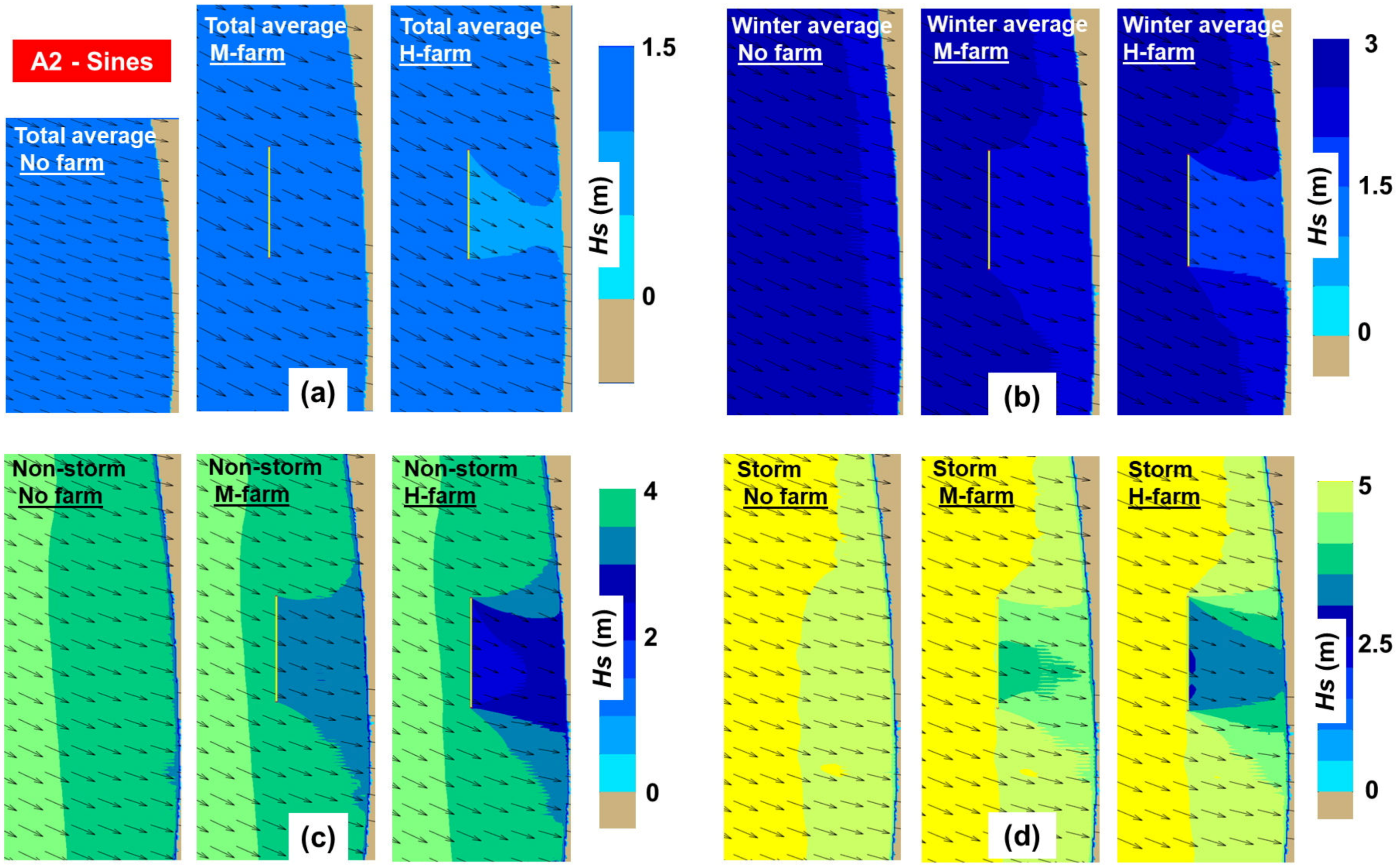
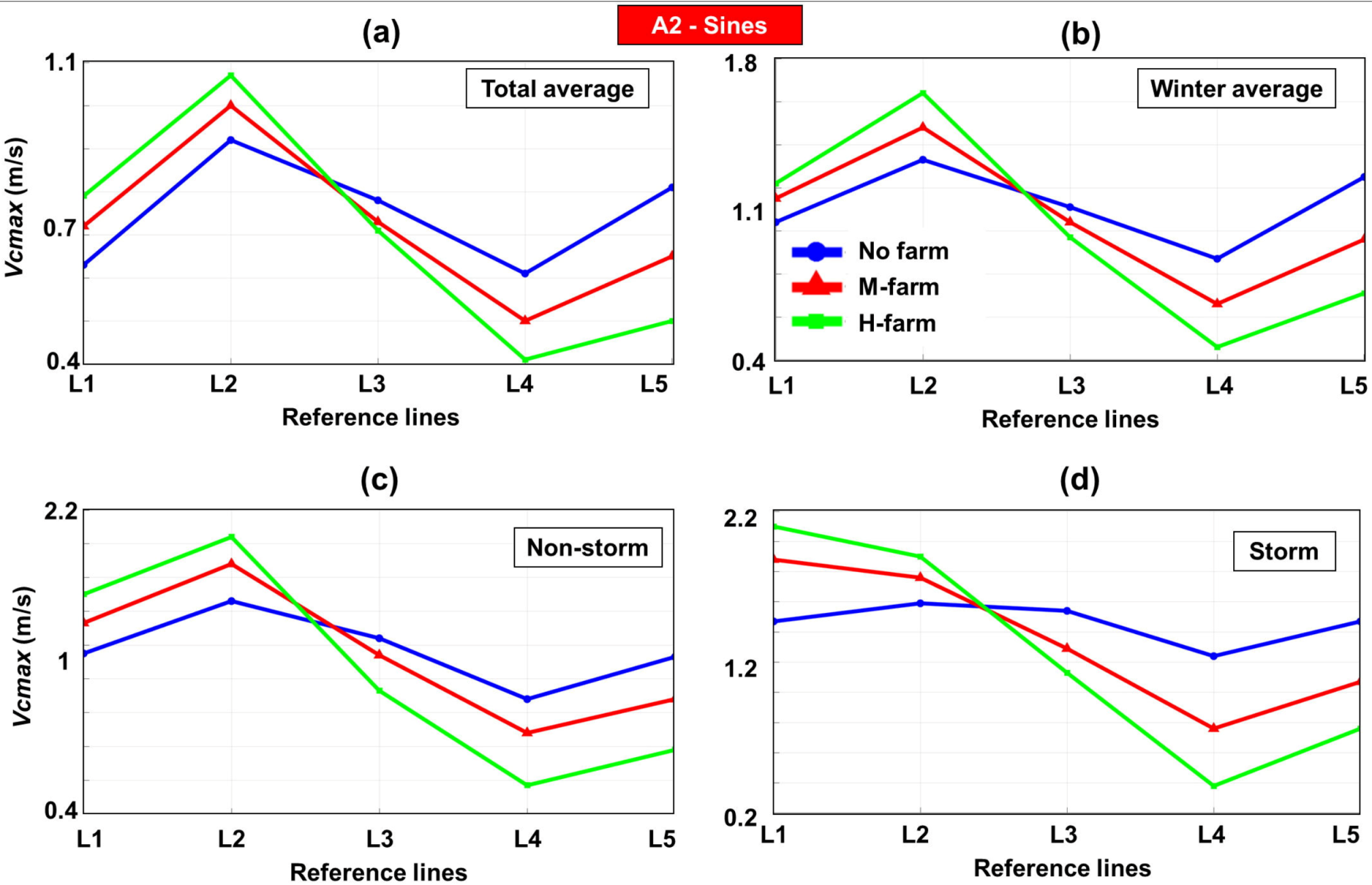
3.1.2. Sines (North Atlantic)

Figure 4 and

Table 5. Sines case study—variation of the wave parameters in the presence of the marine energy farm corresponding to the five nearshore points. The results are indicated for all the case studies considered, where: (a) Hs (significant wave height); (b) wave force; (c) Vbot (orbital velocity at the bottom) values.

Scenario	(a) Hs values (m)
	Total average					Winter average
No farm	1.31	1.33	1.30	1.32	1.34	2.45	2.48	2.42	2.46	2.48
M-farm	1.25	1.18	1.13	1.18	1.26	2.33	2.17	2.09	2.17	2.33
H-farm	1.20	1.04	0.98	1.04	1.19	2.22	1.88	1.78	1.92	2.21
	Non-storm					Storm
No farm	3.63	3.64	3.57	3.61	3.64	4.87	4.81	4.74	4.77	4.78
M-farm	3.45	3.16	3.04	3.16	3.43	4.62	4.11	3.99	4.16	4.54
H-farm	3.30	2.72	2.57	2.78	3.26	4.41	3.47	3.31	3.65	4.36
	(b) Force values (N/m2)
	Total average					Winter average
No farm	0.24	0.18	0.22	0.19	0.18	1.03	0.91	1.03	0.93	0.94
M-farm	0.22	0.14	0.17	0.15	0.16	0.94	0.72	0.77	0.73	0.80
H-farm	0.20	0.12	0.13	0.12	0.14	0.94	0.57	0.58	0.58	0.70
	Non-storm					Storm
No farm	2.52	2.37	2.64	2.33	2.53	4.90	5.13	5.44	4.74	5.73
M-farm	2.32	1.87	1.95	1.77	2.16	4.50	3.98	4.05	3.59	4.96
H-farm	2.15	1.48	1.43	1.40	1.88	4.15	3.08	2.87	2.80	4.36
	(c) Vbot values (m/s)
	Total average					Winter average
No farm	0.23	0.19	0.23	0.20	0.18	0.54	0.46	0.54	0.48	0.44
M-farm	0.22	0.17	0.20	0.18	0.17	0.51	0.39	0.46	0.42	0.41
H-farm	0.21	0.14	0.17	0.16	0.16	0.49	0.34	0.39	0.37	0.39
	Non-storm					Storm
No farm	0.91	0.78	0.90	0.82	0.75	1.40	1.20	1.40	1.30	1.20
M-farm	0.86	0.67	0.76	0.71	0.70	1.30	1.00	1.20	1.10	1.10
H-farm	0.82	0.57	0.63	0.62	0.67	1.30	0.87	0.95	0.96	1.10
	NP1	NP2	NP3	NP4	NP5	NP1	NP2	NP3	NP4	NP5
	Reference points					Reference points

present the variation of the Sines wave conditions in a geographical space and near the NP points. From the spatial distribution of the total average conditions, we notice that a marine energy farm defined by a high absorption property will have a visible impact. By looking at the values corresponding to the nearshore points, we notice that the point NP2 reveals a decrease from 1.33 to 1.18 m in the case of the total average/M-farm.

Regarding the other wave conditions, the spatial variations are similar to those corresponding to the Leixoes area. As for the nearshore points, more important variations correspond to the non-storm and storm conditions, being noticed a maximum attenuation of 1.34 m in the case of the point NP2. The variations of the forces is more significant near the points NP2, NP3 and NP4, while in the case of the parameter Vbot the site NP2 indicates in general lower values, regardless of the scenarios considered for assessment.

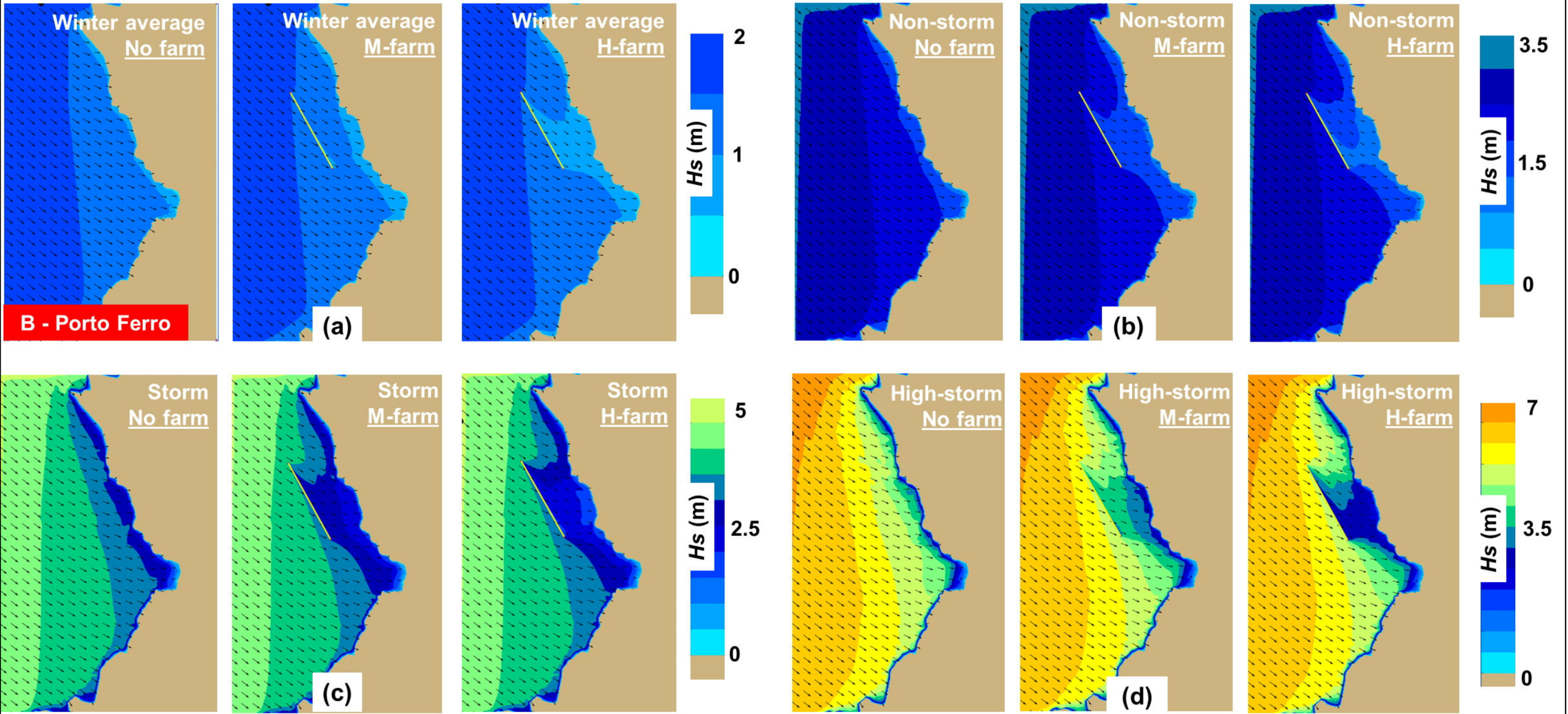
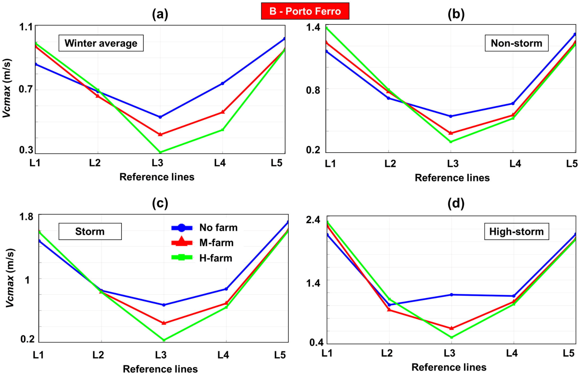
3.1.3. Porto Ferro (Mediterranean Sea)

Going from the North Atlantic Ocean to the Mediterranean Sea, in Figure 5 is presented the western part of the island of Sardinia, where a generic marine energy farm was considered north of the Porto Ferro inlet. The offshore points located in front of the marine energy farm indicate Hs values of 1.35 m—winter average, 2.4 m—non-storm, 3.55 m—storm or 5 m—high-storm, respectively. For the scenario winter average, the presence of a high absorption wave farm is reflected by a shielding effect that will keep the wave heights below 1 m. A similar pattern is noticed for the rest of the case studies, with the mention that for the high absorption scenario, an additional wave field occurs near the shoreline area. From the analysis of the spatial maps, we see that the wave farm has no impact on the wave conditions encountered near the Porto Ferro inlet (point NP4). Nevertheless, by looking at the values of the significant wave heights illustrated in

Table 6. Porto Ferro case study—variation of the wave parameters in the presence of the marine energy farm corresponding to the five nearshore points. The results are indicated for all the case studies considered, where: (a) Hs (significant wave height); (b) wave force; (c) Vbot (orbital velocity at the bottom) values.

Scenario	(a) Hs values (m)
	Winter average					Non-storm
No farm	1.25	1.19	1.18	1.09	1.31	2.16	2.02	1.99	1.94	2.27
M-farm	1.19	1.00	1.06	1.03	1.28	2.04	1.68	1.81	1.81	2.23
H-farm	1.14	0.86	1.01	1.01	1.27	1.94	1.41	1.73	1.78	2.22
	Storm					High-storm
No farm	3.17	2.93	2.92	2.92	3.35	4.43	4.02	4.16	3.66	4.73
M-farm	2.99	2.39	2.63	2.77	3.30	4.18	3.22	3.73	3.59	4.67
H-farm	2.83	2.00	2.52	2.73	3.29	3.97	2.65	3.55	3.57	4.66
	(b) Force values (N/m2)
	Winter average					Non-storm
No farm	0.30	0.14	0.13	0.46	0.04	2.08	0.90	0.87	2.29	0.36
M-farm	0.27	0.10	0.10	0.40	0.03	1.86	0.62	0.73	1.93	0.34
H-farm	0.25	0.07	0.09	0.38	0.03	1.68	0.43	0.66	1.83	0.33
	Storm					High-storm
No farm	6.69	2.91	2.75	1.29	1.48	17.80	6.66	5.80	13.20	4.78
M-farm	5.91	1.90	2.30	2.61	1.42	15.50	4.39	5.03	10.50	4.72
H-farm	5.32	1.28	2.13	2.90	1.41	14.00	2.99	4.65	9.58	4.71
	(c) Vbot values (m/s)
	Winter average					Non-storm
No farm	0.11	0.09	0.08	0.34	0.05	0.32	0.29	0.26	0.77	0.20
M-farm	0.10	0.08	0.07	0.31	0.05	0.31	0.23	0.23	0.71	0.19
H-farm	0.10	0.07	0.07	0.31	0.05	0.29	0.19	0.22	0.70	0.19
	Storm					High-storm
No farm	0.62	0.55	0.51	1.30	0.42	1.10	0.97	0.96	1.80	0.83
M-farm	0.58	0.44	0.46	1.20	0.41	1.10	0.78	0.87	1.80	0.83
H-farm	0.55	0.36	0.44	1.20	0.41	1.00	0.63	0.82	1.70	0.83
	NP1	NP2	NP3	NP4	NP5	NP1	NP2	NP3	NP4	NP5
	Reference points					Reference points

a, we notice that the significant wave height presents some changes. For this point, the Hs values decrease from 1.09 (winter average/no farm) to 1.01 m (winter average/H-farm) or from 3.66 (high-storm/no farm) to 3.57 m (high storm/H-farm), respectively.

The wave forces (Table 6b) present some attenuation in the presence of the marine energy farm, with the noticed values being in the range of 2.99–17.8 N/m² for the high-storm scenario. As for the Vbot values (Table 6c), most of the values do not exceed 1 m/s, with more important values being noticed close to the point NP4 (Porto Ferro inlet).

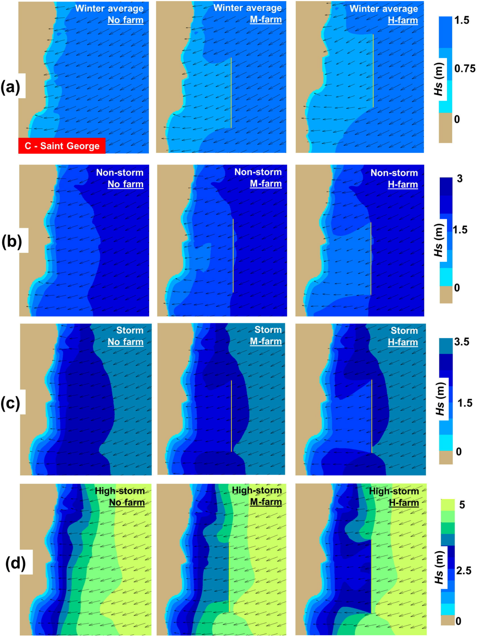
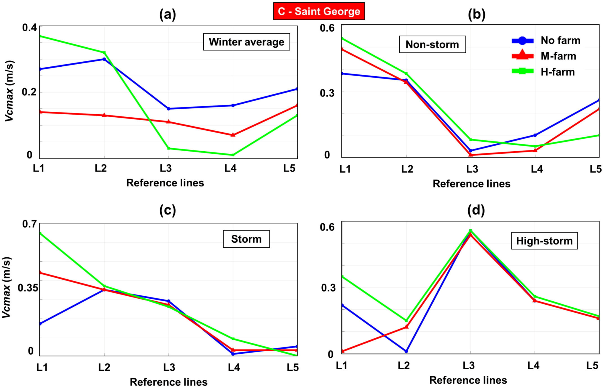
3.1.4. Saint George (Black Sea)

Another area considered for evaluation is the Saint George sector (north-west of the Black Sea, close to the Danube Delta); the Hs spatial distribution is presented in Figure 6. In this case, the coastline is located on the left side, while the dominant direction of the incoming waves is from the north-east (60°). For the winter average conditions, the offshore points indicate values close to 1.19 m, while the significant wave heights behind the wave farm present values in the range of 0.69–0.93 m. In the case of non-storm, the offshore points indicate a maximum significant wave height value of 2.06 m, while at the contact with the WEC line the Hs parameter is reduced by up to 1.17 m.

Moving to the nearshore area, the significant wave heights are influenced by the presence of a marine energy farm, as can be observed in

Table 7. Saint George case study—variation of the wave parameters in the presence of the marine energy farm corresponding to the five nearshore points. The results are indicated for all the case studies considered, where: (a) Hs (significant wave height); (b) wave force; (c) Vbot (orbital velocity at the bottom) values.

Scenario	(a) Hs values (m)
	Winter average					Non-storm
No farm	1.02	1.01	0.98	0.90	0.92	1.84	1.76	1.73	1.61	1.60
M-farm	0.95	0.86	0.83	0.81	0.88	1.72	1.48	1.50	1.46	1.55
H-farm	0.89	0.72	0.69	0.73	0.84	1.62	1.22	1.25	1.32	1.51
	Storm					High-storm
No farm	2.21	2.44	2.11	2.15	1.96	2.37	2.82	2.30	2.35	2.12
M-farm	2.15	2.12	2.03	2.10	1.95	2.34	2.69	2.29	2.34	2.12
H-farm	2.09	1.72	1.85	1.99	1.95	2.28	2.35	2.25	2.31	2.12
	(b) Force values (N/m2)
	Winter average					Non-storm
No farm	0.44	0.35	0.36	0.08	0.55	0.78	1.21	0.93	0.22	0.52
M-farm	0.38	0.27	0.25	0.06	0.50	1.06	0.97	0.82	0.21	0.79
H-farm	0.34	0.20	0.16	0.06	0.45	1.13	0.72	0.58	0.23	0.96
	Storm					High-storm
No farm	3.13	1.80	4.47	1.12	4.48	5.58	7.96	8.04	2.23	7.90
M-farm	2.60	0.99	3.26	0.74	4.33	4.70	5.89	7.64	2.19	7.89
H-farm	1.93	1.47	0.93	0.34	4.18	4.01	0.58	6.87	2.11	7.88
	(c) Vbot values (m/s)
	Winter average					Non-storm
No farm	0.50	0.42	0.51	0.40	0.52	1.00	0.87	1.00	0.84	1.00
M-farm	0.47	0.35	0.43	0.35	0.50	0.98	0.73	0.89	0.76	0.99
H-farm	0.44	0.29	0.35	0.32	0.48	0.92	0.60	0.74	0.69	0.96
	Storm					High-storm
No farm	1.30	1.30	1.30	1.20	1.30	1.50	1.60	1.50	1.40	1.50
M-farm	1.30	1.10	1.30	1.20	1.30	1.50	1.60	1.50	1.40	1.50
H-farm	1.30	0.92	1.20	1.10	1.30	1.50	1.40	1.50	1.40	1.50
	NP1	NP2	NP3	NP4	NP5	NP1	NP2	NP3	NP4	NP5
	Reference points					Reference points

a. For the scenario winter average, the reference points NP2, NP3 and NP4 indicate attenuation that reaches a maximum value of 0.3 m in the case of a high absorbing farm, while a variation of 0.2 m is noticed in the case of the moderate scenario. In the case of non-storm, a maximum difference of 0.54 m (point NP2) is noticed between the no farm situation and non-storm/H-farm, while for the same point the differences reach maximum values of 0.72 (storm) or 0.47 m (high-storm), respectively. The wave forces (Table 7b) indicate, in general, lower values close to the point NP4, with values below 0.25 N/m² being noticed for the scenarios winter average and non-storm, while a maximum of 2.23 N/m² is noticed in the case of the scenario high-storm/no farm. The Vbot values corresponding to the no farm scenario gradually increase from a minimum of 0.4 m/s (winter average) up to maximum of 1 (non-storm), (storm) or 1.6 m/s (high-storm), respectively. Compared to other sites, the point NP2 indicates more important variations.

3.2. Assessment of the Longshore Currents

It is well known that coastal areas are also influenced by the presence of the longshore currents [55,56]. These currents are generated by the breaking waves that enter in the surf area, it being expected that in the case of storm events the current velocity will indicate higher values. Figure 7 is focused on such an analysis that illustrates the longshore current distribution in the Leixoes sector, in this case indicating the maximum value of the current velocity (Vcmax in m/s) along the L-lines. From the analysis of these case studies, we can notice that various patterns can be identified.

Figure 8 illustrates the velocity distribution for the Sines sector. Regardless of the case study considered, a pattern is noticed where the presence of the marine energy farm enhances the current velocity near the lines L1 and L2, while an opposite effect is noticed for the lines L3, L4 and L5, respectively. The minimum and maximum peaks are accounted for by the high absorption configuration, which goes from 0.38 to 2.1 m/s in the case of a storm event.

Figure 9 presents the velocity distribution for the Porto Ferro area. In this case, more important variations are noticed close to the line L3, where the presence of a wave farm decreases the current velocity to a minimum of 0.2 m/s (non-storm/H-farm and storm/H-farm).

The line L2 indicates no significant variation, regardless of the case study considered, while as we go to the scenarios storm and high-storm it appears that a marine energy farm will not have a big impact on the nearshore currents (excepting the line L3). In addition, it is important to mention that for the case studies winter average and non-storm, the velocity will increase along the line L1, reaching maximum values of 0.99 (winter average) or 1.37 m/s (non-storm), respectively.

Figure 10 illustrates the maximum values of the current velocity along the reference lines, by considering this time the Saint George area. By looking at these results, we notice that mixed patterns occur for each case study. Thus, in the case of the line L1, the velocity corresponding to the case studies winter average and high-storm increases in the presence of a high absorber farm and decreases for a moderate one. For the scenario winter average/no farm, the current velocity decreases near the lines L3, L4 and L5, reaching minimum values of 0.07 m/s for winter average/M-farm and 0.01 m/s for winter average/H-farm. Since the wave direction is a crucial parameter in the development of the nearshore currents, the fact that the marine energy farm may produce significant changes in terms of wave direction may also affect the longshore current velocity. That is why, although the waves lose energy in the presence of the marine energy farm, in certain situations, due to such changes in wave direction, the longshore current velocity can increase down-wave from a marine energy farm. A similar situation was identified in [33], for various wave conditions.

For the non-storm situation, the current velocity will increase near the line L1, while an opposite trend is noticed close to the lines L4 and L5. Smaller fluctuations are noticed near the lines L2 and L3, while a similar situation is reported by the scenario storm (L2, L3, L5) or by high-storm (L3, L4, L5).

4. Discussion of the Results

The current approaches for coastal protection mainly involve seawalls and breakwaters. Since the aim of a WEC farm is to extract energy from the waves, a wave farm represents a very suitable alternative. Nevertheless, such farms are not beneficial in every environment, as is the case of enclosed seas, which do not represent the best option for the development of a wave project. This is because the wave conditions are significantly reduced compared to the ocean environment. On the other hand, Europe is an active player in the development of the WEC systems [57,58,59,60], and since a large part of this region is surrounded by semi-enclosed seas, there are higher chances to see marine farms operating in these waters in the future.

In any coastal area, the sediment transport is divided between bedload and suspended load, it being estimated that the most important hydraulic parameter for littoral transport is represented by the wave conditions. The littoral drift is influenced by several parameters (significant wave height; wave direction; grain size, etc.) which can be used to determine the littoral transport rate, denoted with Q (m³/24 hrs) [61]. For example, in the case of an incident angle of 30° (like the one considered in the present work – see Table 1), the transport rate of a beach sand is associated with the following values: Hs = 1 m; Q = 300 m³/24 hrs; Hs = 3 m; Q = 10,000 m³/24 hrs; Hs = 5 m; Q = 65,000 m³/24 hrs. This assumption can be applied for most of the target areas, taking into account that the Saint George sector is defined by quartz sands (medium-fine sands), with a similar situation being noticed for the Sines area, where the local rivers represent the main source of sediments [33,38].

By interpolating the results presented in reference [61], it is possible to assess the transport rate corresponding to the nearshore points (from NP1 to NP5), assuming that the wave conditions are considered for a time interval of 24 h.

Table 8. Transport rate of the beach sand considering the scenario when the incident wave angle is 30°. The results are presented for all the target areas considered: Leixoes, Sines, Porto Ferro and Saint George.

Leixoes	*	total average/NP5	winter average/NP4	non-storm/NP4	storm/NP4
	**	759	5680	23,200	62,900
	***	M-farm—15.7%; H-farm—22.4%	M-farm—60.6%; H-farm—74.4%	M-farm—52.6%; H-farm—72.4%	M-farm—40.6%; H-farm—66.3%
Sines	*	total average/NP5	winter average/NP2	non-storm/NP2	storm/NP1
	**	878	5840	22,800	60,450
	***	M-farm—15.5% H-farm—29%	M-farm—42.5% H-farm—69.2%	M-farm—42.1 H-farm—66%	M-farm—14.5% H-farm—67.9%
Porto Ferro	*	winter average/NP5	non-storm/NP5	storm/NP5	high-storm/NP5
	**	827	4160	17,000	55,560
	***	M-farm—6.2% H-farm—8.2%	M-farm—7.7% H-farm—9.6%	M-farm—5.9% H-farm—7.1%	M-farm—3.7% H-farm—4.3%
Saint George	*	winter average/NP3	non-storm/NP3	storm/NP3	high-storm/NP3
	**	294	1541	2880	4400
	***	M-farm—15.3% H-farm—29.6%	M-farm—25.4% H-farm—53%	M-farm—22.2% H-farm—39.4%	M-farm—1.8% H-farm—9.1%

* Wave conditions and reference points; ** No farm—(Q in m³/24 hrs); *** Wave farm (Q attenuation in %).

present the transport rates for some representative nearshore points. According to these results, we can notice that even small changes in the wave heights may lead to a significant reduction in the littoral transport rate generated by the wave action.

In this work, the longshore current velocity represents another parameter considered for investigation, which was assessed in each target area (from Figure 7, Figure 8, Figure 9 and Figure 10). The Hjulström curve [62,63] is frequently used by hydrologists to determine if a river will transport/deposit sediment or will erode by taking into account the water velocity and the sediment particle size. If the water velocity is below 3 m/s, the sediment will be transported or deposited based on their size (<0.01 mm—transportation), while after this threshold the erosion processes may occur. At this point, it is important to mention that the Hjulström diagram is able to provide only a first-order analysis of the interaction between flowing water and sediments. From the analysis of the results in the Leixoes area, we notice that the erosion process may occur in the sector located close to the line L1, where in fact the presence of the farm increases the current velocity. For the scenarios total average, winter average and non-storm, a marine energy farm significantly reduces the current velocity for the lines L4 and L5, contributing in this way to the protection of the coastline. Regarding the Sines area, a marine energy farm may increase the erosion processes in the upper part of the shielded region (lines L1 and L2) and will significantly decrease the current velocity in the lower part (lines L4 and L5).

As for the Porto Ferro area, by looking at the results corresponding to the high-storm scenario, we notice that near the line L3, the current velocity reduces. This does not necessarily mean that this sector will be protected, taking into account that the wave farm has no impact on the current velocity reported in the adjacent sectors. Regarding the expected values from the Saint George sector, we notice that they cannot be considered a source of coastal erosion, being assumed to be involved more in the sediment flow. For this sector, the coastal erosion will probably be more directly related to the wave action that can be generated during a storm event (storm and high-storm), with orbital velocities in the range of 1.3 and 1.5 m/s.

5. Conclusions

The objective of the present work is to identify the expected impact of a generic marine energy farm that would be implemented in various coastal environments, such as the Portuguese coast, Sardinia or in the north-western part of the Black Sea (close to the Danube Delta). The idea is to use the layout of a single marine energy farm, namely 3 km in length and located at about 2 km from the shoreline, in order to determine what will be the shoreline impact for a moderate and high absorption scenario.

According to these results, it was found that although from the analysis of the spatial maps there was reported no significant variation in the Hs values in the case of the first two scenarios (e.g., Portuguese coast—total average and winter average), according to the nearshore reference points, the influence of a WEC line is visible, and thus significant variations close to the shoreline are expected. From the analysis of the Hs values corresponding to the Sines and Leixoes areas, it was noticed that the Sines sector indicates in general many resources close to the shoreline, although the considered case studies are identical. A more complete picture of the nearshore impact was provided by including some other relevant parameters, such as the wave forces and the orbital velocity that may occur near the NP-points. Regardless of the considered target area, it was noticed that these two parameters increase as the wave conditions become more energetic. By looking at these results, we can say that, in general, the Leixoes area indicate much higher values, being followed by the Saint George sector in the Black Sea.

In terms of the current velocity, with the exception of the Saint George sector, it is possible that during an extreme event (e.g., storm), the longshore currents generated by the breaking waves affect the coastal stability by eroding the sediment deposits and transporting in other beach sectors the sediment transported by the waves. For the Saint George sector, it is more likely that the erosion processes are associated with to the hydraulic action of the waves and to the fact that the large dams build on the Danube River significantly reduces the volume of alluvia.

Since at this moment there are no operational wave farms, it is difficult to say what the configuration of such a project will be, and as a consequence throughout various ‘’what-if’’ case studies it is possible to estimate the expected implications for the coastal protection. Finally, we can mention that the results from the present work are in the line with the current research that considers hybrid modelling systems, which combine the output of a wave model with other simulation tools (ex: sediment transport; longshore currents).

References

1. Rangel-Buitrago, N.; Williams, A.T.; Anfuso, G. Hard protection structures as a principal coastal erosion management strategy along the Caribbean coast of Colombia. A chronicle of pitfalls. Ocean. Coast. Manag. 2018, 156, 58–75. [Google Scholar] [CrossRef]
2. Octifanny, Y.; Hudalah, D. Agglomeration and Extension in Northern Coast of West Java: A Transformation into Mega Region, Proceedings of the Cities 2016 International Conference: Coastal Planning for Sustainable Maritime Development, Sepuluh, Indonesia, 18 October 2016; Iop Publishing Ltd.: Bristol, UK, 2017; Volume 79. [Google Scholar]
3. Smee, D.L. Coastal Ecology: Living Shorelines Reduce Coastal Erosion. Curr. Biol. 2019, 29, R411–R413. [Google Scholar] [CrossRef] [PubMed]
4. Jeong, H.Y. A Study on Changes in Coastal Erosion Environment by Time Series Coastal Detection Using GIS. J. Coast. Res. 2019, 331–335. [Google Scholar] [CrossRef]
5. Nguyen, H.T.L.; Luong, H.P.V. Erosion and deposition processes from field experiments of hydrodynamics in the coastal mangrove area of Can Gio, Vietnam. Oceanologia 2019, 61, 252–264. [Google Scholar] [CrossRef]
6. Valderrama-Landeros, L.; Flores-de-Santiago, F. Assessing coastal erosion and accretion trends along two contrasting subtropical rivers based on remote sensing data. Ocean. Coast. Manag. 2019, 169, 58–67. [Google Scholar] [CrossRef]
7. Rangel-Buitrago, N.; de Jonge, V.N.; Neal, W. How to make Integrated Coastal Erosion Management a reality. Ocean. Coast. Manag. 2018, 156, 290–299. [Google Scholar] [CrossRef]
8. Martinez, C.; Contreras-Lopez, M.; Winckler, P.; Hidalgo, H.; Godoy, E.; Agredano, R. Coastal erosion in central Chile: A new hazard? Ocean. Coast. Manag. 2018, 156, 141–155. [Google Scholar] [CrossRef]
9. Bosello, F.; De Cian, E. Climate change, sea level rise, and coastal disasters. A review of modeling practices. Energy Econ. 2014, 46, 593–605. [Google Scholar] [CrossRef] [Green Version]
10. Ahmad, N.; Bihs, H.; Chella, M.A.; Kamath, A.; Arntsen, O.A. CFD Modeling of Arctic Coastal Erosion due to Breaking Waves. Int. J. Offshore Polar Eng. 2019, 29, 33–41. [Google Scholar] [CrossRef] [Green Version]
11. Fourie, J.-P.; Ansorge, I.; Backeberg, B.; Cawthra, H.C.; MacHutchon, M.R.; van Zyl, F.W. The influence of wave action on coastal erosion along Monwabisi Beach, Cape Town. S. Afr. J. Geomat. 2015, 4, 96–109. [Google Scholar] [CrossRef]
12. Harley, M.D.; Turner, I.L.; Kinsela, M.A.; Middleton, J.H.; Mumford, P.J.; Splinter, K.D.; Phillips, M.S.; Simmons, J.A.; Hanslow, D.J.; Short, A.D. Extreme coastal erosion enhanced by anomalous extratropical storm wave direction. Sci Rep. 2017, 7, 6033. [Google Scholar] [CrossRef] [PubMed] [Green Version]
13. Bacino, G.L.; Dragani, W.C.; Codignotto, J.O. Changes in wave climate and its impact on the coastal erosion in Samborombon Bay, Rio de la Plata estuary, Argentina. Estuar. Coast. Shelf Sci. 2019, 219, 71–80. [Google Scholar] [CrossRef]
14. Feagin, R.A.; Furman, M.; Salgado, K.; Martinez, M.L.; Innocenti, R.A.; Eubanks, K.; Figlus, J.; Huff, T.P.; Sigren, J.; Silva, R. The role of beach and sand dune vegetation in mediating wave run up erosion. Estuar. Coast. Shelf Sci. 2019, 219, 97–106. [Google Scholar] [CrossRef]
15. Serafim, M.B.; Siegle, E.; Corsi, A.C.; Bonetti, J. Coastal vulnerability to wave impacts using a multi-criteria index: Santa Catarina (Brazil). J. Environ. Manage. 2019, 230, 21–32. [Google Scholar] [CrossRef] [PubMed]
16. Kerguillec, R.; Audere, M.; Baltzer, A.; Debaine, F.; Fattal, P.; Juigner, M.; Launeau, P.; Le Mauff, B.; Luquet, F.; Maanan, M.; et al. Monitoring and management of coastal hazards: Creation of a regional observatory of coastal erosion and storm surges in the pays de la Loire region (Atlantic coast, France). Ocean. Coast. Manag. 2019, 181, 104904. [Google Scholar] [CrossRef]
17. Montreuil, A.-L.; Chen, M.; Elyahyioui, J. Assessment of the impacts of storm events for developing an erosion index. Reg. Stud. Mar. Sci. 2017, 16, 124–130. [Google Scholar] [CrossRef]
18. Schoonees, T.; Mancheno, A.G.; Scheres, B.; Houma, T.J.; Silva, R.; Schlurmann, T.; Schuettrumpf, H. Hard Structures for Coastal Protection, Towards Greener Designs. Estuaries Coasts 2019, 42, 1709–1729. [Google Scholar] [CrossRef]
19. Andre, C.; Boulet, D.; Rey-Valette, H.; Rulleau, B. Protection by hard defence structures or relocation of assets exposed to coastal risks: Contributions and drawbacks of cost-benefit analysis for long-term adaptation choices to climate change. Ocean. Coast. Manag. 2016, 134, 173–182. [Google Scholar] [CrossRef]
20. Zhang, X.; Lu, K.; Yin, P.; Zhu, L. Current and future mudflat losses in the southern Huanghe Delta due to coastal hard structures and shoreline retreat. Coast. Eng. 2019, 152, 103530. [Google Scholar] [CrossRef]
21. Firth, L.B.; Thompson, R.C.; Bohn, K.; Abbiati, M.; Airoldi, L.; Bouma, T.J.; Bozzeda, F.; Ceccherelli, V.U.; Colangelo, M.A.; Evans, A.; et al. Between a rock and a hard place: Environmental and engineering considerations when designing coastal defence structures. Coast. Eng. 2014, 87, 122–135. [Google Scholar] [CrossRef] [Green Version]
22. Liu, X.; Wang, Y.; Costanza, R.; Kubiszewski, I.; Xu, N.; Gao, Z.; Liu, M.; Geng, R.; Yuan, M. Is China’s coastal engineered defences valuable for storm protection? Sci. Total Environ. 2019, 657, 103–107. [Google Scholar] [CrossRef] [PubMed]
23. Pranzini, E. Shore protection in Italy: From hard to soft engineering… and back. Ocean. Coast. Manag. 2018, 156, 43–57. [Google Scholar] [CrossRef]
24. Williams, A.T.; Rangel-Buitrago, N.; Pranzini, E.; Anfuso, G. The management of coastal erosion. Ocean. Coast. Manag. 2018, 156, 4–20. [Google Scholar] [CrossRef]
25. Rusu, E.; Onea, F. Hybrid Solutions for Energy Extraction in Coastal Environment. Energy Procedia 2017, 118, 46–53. [Google Scholar] [CrossRef]
26. Zhang, H.; Aggidis, G.A. Nature rules hidden in the biomimetic wave energy converters. Renew. Sustain. Energy Rev. 2018, 97, 28–37. [Google Scholar] [CrossRef] [Green Version]
27. Aderinto, T.; Li, H. Ocean Wave Energy Converters: Status and Challenges. Energies 2018, 11, 1250. [Google Scholar] [CrossRef] [Green Version]
28. Franzitta, V.; Curto, D. Sustainability of the Renewable Energy Extraction Close to the Mediterranean Islands. Energies 2017, 10, 283. [Google Scholar] [CrossRef] [Green Version]
29. Khalifehei, K.; Azizyan, G.; Gualtieri, C. Analyzing the Performance of Wave-Energy Generator Systems (SSG) for the Southern Coasts of Iran, in the Persian Gulf and Oman Sea. Energies 2018, 11, 3209. [Google Scholar] [CrossRef] [Green Version]
30. Bento, A.R.; Rusu, E.; Martinho, P.; Guedes Soares, C. Assessment of the changes induced by a wave energy farm in the nearshore wave conditions. Comput. Geosci. 2014, 71, 50–61. [Google Scholar] [CrossRef]
31. Rusu, E.; Onea, F. Evaluation of the shoreline effect of the marine energy farms in different coastal environments. In Proceedings of the 2018 3rd International Conference on Advances on Clean Energy Research (ICACER 2018), Barcelona, Spain, 6–8 April 2018; Cui, W., Rusu, E., Eds.; 2018; Volume 51, p. UNSP 03005. [Google Scholar]
32. Zanopol, A.T.; Onea, F.; Rusu, E. Evaluation of the Coastal Influence of a Generic Wave Farm Operating in the Romanian Nearshore. J. Environ. Prot. Ecol. 2014, 15, 597–605. [Google Scholar]
33. Rusu, E.; Onea, F. Study on the influence of the distance to shore for a wave energy farm operating in the central part of the Portuguese nearshore. Energy Conv. Manag. 2016, 114, 209–223. [Google Scholar] [CrossRef]
34. Onea, F.; Rusu, E. The expected efficiency and coastal impact of a hybrid energy farm operating in the Portuguese nearshore. Energy 2016, 97, 411–423. [Google Scholar] [CrossRef]
35. Diaconu, S.; Rusu, E. The Environmental Impact of a Wave Dragon Array Operating in the Black Sea. Sci. World J. 2013, 498013. [Google Scholar] [CrossRef] [PubMed] [Green Version]
36. Rusu, E.; Guedes Soares, C. Coastal impact induced by a Pelamis wave farm operating in the Portuguese nearshore. Renew. Energy 2013, 58, 34–49. [Google Scholar] [CrossRef]
37. Millar, D.L.; Smith, H.C.M.; Reeve, D.E. Modelling analysis of the sensitivity of shoreline change to a wave farm. Ocean. Eng. 2007, 34, 884–901. [Google Scholar] [CrossRef]
38. Zanopol, A.T.; Onea, F.; Rusu, E. Coastal impact assessment of a generic wave farm operating in the Romanian nearshore. Energy 2014, 72, 652–670. [Google Scholar] [CrossRef]
39. Abanades, J.; Greaves, D.; Iglesias, G. Coastal defence through wave farms. Coast. Eng. 2014, 91, 299–307. [Google Scholar] [CrossRef] [Green Version]
40. Bergillos, R.J.; Rodriguez-Delgado, C.; Iglesias, G. Wave farm impacts on coastal flooding under sea-level rise: A case study in southern Spain. Sci. Total Environ. 2019, 653, 1522–1531. [Google Scholar] [CrossRef]
41. Mendoza, E.; Silva, R.; Zanuttigh, B.; Angelelli, E.; Andersen, T.L.; Martinelli, L.; Norgaard, J.Q.H.; Ruol, P. Beach response to wave energy converter farms acting as coastal defence. Coast. Eng. 2014, 87, 97–111. [Google Scholar] [CrossRef]
42. Astariz, S.; Iglesias, G. Output power smoothing and reduced downtime period by combined wind and wave energy farms. Energy 2016, 97, 69–81. [Google Scholar] [CrossRef]
43. Astariz, S.; Iglesias, G. Accessibility for operation and maintenance tasks in co-located wind and wave energy farms with non-uniformly distributed arrays. Energy Conv. Manag. 2015, 106, 1219–1229. [Google Scholar] [CrossRef]
44. Carballo, R.; Arean, N.; Alvarez, M.; Lopez, I.; Castro, A.; Lopez, M.; Iglesias, G. Wave farm planning through high-resolution resource and performance characterization. Renew. Energy 2019, 135, 1097–1107. [Google Scholar] [CrossRef]
45. Castro-Santos, L.; Silva, D.; Rute Bento, A.; Salvacao, N.; Guedes Soares, C. Economic Feasibility of Wave Energy Farms in Portugal. Energies 2018, 11, 3149. [Google Scholar] [CrossRef] [Green Version]
46. Rodriguez-Delgado, C.; Bergillos, R.J.; Ortega-Sanchez, M.; Iglesias, G. Wave farm effects on the coast: The alongshore position. Sci. Total Environ. 2018, 640, 1176–1186. [Google Scholar] [CrossRef] [PubMed]
47. Stokes, C.; Conley, D.C. Modelling Offshore Wave farms for Coastal Process Impact Assessment: Waves, Beach Morphology, and Water Users. Energies 2018, 11, 2517. [Google Scholar] [CrossRef] [Green Version]
48. Onea, F.; Rusu, E. The Expected Shoreline Effect of a Marine Energy Farm Operating Close to Sardinia Island. Water 2019, 11, 2303. [Google Scholar] [CrossRef] [Green Version]
49. Rusu, E.; Soares, C.G. Validation of Two Wave and Nearshore Current Models. J. Waterw. Port. Coast. Ocean. Eng. 2010, 136, 27–45. [Google Scholar] [CrossRef]
50. Rusu, E.; Conley, D.; Ferreira-Coelho, E. A hybrid framework for predicting waves and longshore currents. J. Mar. Syst. 2008, 69, 59–73. [Google Scholar] [CrossRef]
51. Rusu, E.; Macuta, S. Numerical Modelling of Longshore Currents in Marine Environment. Environ. Eng. Manag. J. 2009, 8, 147–151. [Google Scholar] [CrossRef]
52. Booij, N.; Ris, R.C.; Holthuijsen, L.H. A third-generation wave model for coastal regions: 1. Model description and validation. J. Geophys. Res. 1999, 104, 7649–7666. [Google Scholar] [CrossRef] [Green Version]
53. Mettlach, T.R.; Earle, M.D.; Hsu, Y.L. Software Design Document for the Navy Standard Surf. Model. Version 3.2; Defense Technical Information Center: Fort Belvoir, VA, USA, 2002. [Google Scholar]
54. Onea, F.; Rusu, L. Coastal Impact of a Hybrid Marine Farm Operating Close to the Sardinia Island. In Proceedings of the OCEANS 2015-Genova, Genoa, Italy, 18–21 May 2015; IEEE: New York, NY, USA. ISBN 978-1-4799-8737-5. [Google Scholar]
55. Rusu, E.; Guedes Soares, C. Wave modelling at the entrance of ports. Ocean. Eng. 2011, 38, 2089–2109. [Google Scholar] [CrossRef]
56. Ivan, A.; Gasparotti, C.; Rusu, E. Influence of the Interactions between Waves and Currents on the Navigation at the Entrance of the Danube Delta. J. Environ. Prot. Ecol. 2012, 13, 1673–1682. [Google Scholar]
57. Rusu, L.; Onea, F. The performance of some state-of-the-art wave energy converters in locations with the worldwide highest wave power. Renew. Sustain. Energy Rev. 2017, 75, 1348–1362. [Google Scholar] [CrossRef]
58. Clement, A.; McCullen, P.; Falcao, A.; Fiorentino, A.; Gardner, F.; Hammarlund, K.; Lemonis, G.; Lewis, T.; Nielsen, K.; Petroncini, S.; et al. Wave energy in Europe: Current status and perspectives. Renew. Sustain. Energy Rev. 2002, 6, 405–431. [Google Scholar] [CrossRef]
59. O’Hagan, A.M.; Huertas, C.; O’Callaghan, J.; Greaves, D. Wave energy in Europe: Views on experiences and progress to date. Int. J. Mar. Energy 2016, 14, 180–197. [Google Scholar] [CrossRef] [Green Version]
60. Sarmento, A.J.N.A.; La Regina, V.; Neumann, F. Europe’s Wave Energy Development: Technological, Economical and Political Viewpoints, Proceedings of the Sixteenth (2006) International Offshore and Polar Engineering Conference, San Francisco, CA, USA, 28 May–2 June 2006; Chung, J.S., Hong, S.W., Marshall, P.W., Komai, T., Koterayama, W., Eds.; International Society Offshore& Polar Engineers: Cupertino, CA, USA, 2006; Volume 1, pp. 1–8. [Google Scholar]
61. Coastal Hydrodynamics and Transport Processes—Coastal Wiki. Available online: http://www.coastalwiki.org/wiki/Coastal_Hydrodynamics_And_Transport_Processes (accessed on 6 March 2020).
62. Bombardelli, F.A.; Moreno, P.A. Exchange at the bed sediments-water column interface. In Fluid Mechanics of Environmental Interfaces, 2nd ed.; Gualtieri, C., Mihailovic, D.T., Eds.; CRC Press/Balkema: Leiden, The Netherlands, 2012; pp. 221–253. ISBN 978-0-415-62156-4. [Google Scholar]
63. Heininger, P.; Cullmann, J. (Eds.) Sediment Matter; Springer: Basel, Switzerland, 2015; ISBN 978-3-319-14696-6. [Google Scholar]
Figure 1. Locations of the target areas considered for assessment, where: (a) Portugal continental (North Atlantic Ocean); (b) Porto Ferro, Sardinia (Mediterranean Sea); (c) Saint George (Black Sea). Figures processed from Google Earth (2019).
Jmse 08 00228 g001
Figure 2. Case studies and computational domains considered for evaluation, where: (a) Leixoes; (b) Sines; (c) Porto Ferro; (d) Saint George. In the foreground, the configurations of the wave farms are presented, while in the background, the bathymetric map is represented [33,34,38,48].
Jmse 08 00228 g002
Figure 3. Leixoes case study—wave conditions (Hs scalar fields and wave vectors) corresponding to: (a) total average; (b) winter average; (c) non-storm; (d) storm.
Jmse 08 00228 g003
Figure 4. Sines case study—variation of the significant wave height and of the mean wave direction related to: (a) total average; (b) winter average; (c) non-storm; (d) storm.
Jmse 08 00228 g004
Figure 5. Porto Ferro study—variation of the significant wave height and wave direction related to: (a) winter average; (b) non-storm; (c) storm; (d) high-storm.
Jmse 08 00228 g005
Figure 6. Saint George case study—variation of the significant wave height and mean wave direction corresponding to: (a) winter average; (b) non-storm; (c) storm; (d) high-storm.
Jmse 08 00228 g006
Figure 7. Leixoes study—maximum current velocity (Vcmax in m/s) estimated along the five reference lines considered (L1–L5). The results are indicated for: (a) total average; (b) winter average; (c) non-storm; (d) storm.
Jmse 08 00228 g007
Figure 8. Sines study—maximum current velocity (Vcmax in m/s) estimated along the five reference lines considered (L1–L5). The results are indicated for: (a) total average; (b) winter average; (c) non-storm; (d) storm.
Jmse 08 00228 g008
Figure 9. Porto Ferro study—maximum current velocity (Vcmax in m/s) estimated along the five reference lines considered (L1–L5). The results are indicated for: (a) winter average; (b) non-storm; (c) storm; (d) high-storm.
Jmse 08 00228 g009
Figure 10. Saint George study—maximum current velocity (Vcmax in m/s) estimated along the five reference lines considered (L1–L5). The results are indicated for: (a) winter average; (b) non-storm; (c) storm; (d) high-storm.
Jmse 08 00228 g010