A Novel Fault Location Approach for Scientific Cabled Seafloor Observatories

Abstract

The maintenance of scientific cabled seafloor observatories (CSOs) is not only extremely difficult but also of high cost for their subsea location. Therefore, the cable fault detection and location are essential and must be carried out accurately. For this purpose, a novel on-line fault location approach based on robust state estimation is proposed, considering state data gross errors in sensor measurements and the influence of temperature on system parameter variation. The circuit theory is used to build state estimation equations and identify the power system topology of faulty CSOs. This method can increase the accuracy of fault location, and reduce the lose form shutting down a faulty CSO in traditional fault location methods. It is verified by computer simulation and the laboratory prototype of a planned CSO in the East China Sea, and the fault location error is proved to be less than 1 km.

1. Introduction

Cabled seafloor observatories (CSOs) are large-scale underwater intelligent sensor networks, which provide scientists with all-weather, long-term, real-time, and in-situ observations of the complex processes operating within the ocean [1].

A CSO consists of undersea stations, optical repeaters, branching units (BUs), backbone and spur electro-optical submarine cables, and shore stations. Each spur cable is connected to the backbone cable through a BU. For long distances of data transmission, optical repeaters are installed in the backbone cables to amplify the fiber-optic signals. Large-scale CSOs can be in various topologies, with submarine cables of hundreds to thousands of kilometers. A typical CSO structure planned to be applied in the East China Sea is shown in Figure 1. In CSOs, the power feeding equipment (PFE) in the shore stations provide up to high voltage direct current (HVDC) rated to 10 kV for the undersea power system. Typical submarine electro-optic cables only have one copper conductor. Thus, anodes are set on the shore stations, and cathodes are set on the undersea stations. In this way, the seawater is used as the current returning path. Each undersea station has a DC/DC converter converting the DC 10 kV into DC 375 V. Undersea stations supply power to science instrument platforms as payloads. Voltage and current sensors are installed on shore stations and both inputs and outputs of undersea stations. The sensors used in CSOs are Hall sensors, and have measurement errors of around 1%.

The designed lifetime of CSOs is at least 25 years. In the lifetime of a CSO, the cable quality or external forces by fishery or anchorage will lead to cable failures [2,3]. The main performance of cable faults is the decreasing of the cable insulation. Cable faults can be divided into low resistance faults and high resistance faults, according to cable insulation levels. A low resistance fault happens when the cable insulation resistance is so low that at least one undersea station cannot start up, because its input voltage is below the startup threshold. When a high resistance fault occurs, all undersea stations can start up, but at least one cannot be fully loaded. Typically, the minimum startup voltage of undersea stations is 50% to 60% of the maximum rated power transmission voltage. As high resistance faults usually happen before low resistance faults, this paper focused on the high resistance fault location.

The voltage and current sensors of shore stations and undersea stations obtain necessary data for fault location, but BUs have no sensors because of the compact size and the lack of sensor date transmission capability [4]. These sensor data with low measurement redundancy usually have gross errors and will affect the fault location accuracy. In addition, seawater temperatures have significant influence on submarine cable resistances, which are important parameters of the state estimation and fault location.

Existing cable fault location methods have been proposed for low resistance faults of backbone cables and multi-terminal CSOs. In the process of fault location, the power supply of shore stations must be shut down first and then started under a low voltage, so that all undersea stations cannot start up [5,6,7,8]. Moreover, these methods can only apply to the CSOs that have at least two shore stations.

In terrestrial power systems, travelling wave methods are most commonly used. They realize fault location according to the time difference of arriving between the initial wave and the reflected waves from the fault point [9,10,11]. As repeaters and BUs in CSOs will reflect the travelling wave, and the wave can only travel several kilometers, these methods are not suitable for CSOs.

In this paper, a novel on-line cable fault location approach, based on robust state estimation, is proposed for high resistance faults of the backbone and spur cable of CSOs.

2. Fault Location in CSOs

2.1. Data Pre-Processing

The state data of the CSO power system is measured by the voltage and current sensors in undersea stations and shore stations. These data have gross errors and will affect fault location accuracy. In order to eliminate the data with gross errors, data pre-processing is used based on the Grubbs criterion [12].

In CSOs, the sampling period of sensors is one second. Every data group of 15 samples is collected to calculate the mean value and the standard deviation. According to the Grubbs criterion, when the residual of the measurement data x_i is satisfied $\left|v_i\right|=\left|x_i-x\right|\ge g\left(n,a\right)·\sigma \left(x\right)$, it is considered to be abnormal and should be deleted. In the above equation, v_i means the residual of the measurement, x means the average of the group data, i means the number of the group data, n means the measurement times in a data group, a means the probability of abandoning true data, and $\sigma \left(x\right)=\sqrt{\frac{{{\displaystyle \sum }}^{}{v}_i^2}{n}}$ means the standard deviation of the group data. When n = 15 and a = 0.05, g(n,a) = 2.41.

This step can ensure the reliability of the data and prepare for parameter estimation.

2.2. Parameter Estimation

The CSOs use submarine cables to transmit the electrical power. The resistance of a submarine cable can be expressed as:

$$R=\frac{\rho L}{S}$$

(1)

In the equation, L means cable length, S means the conductor cross-sectional area, $\rho$ means the resistivity. The relationship between resistivity and temperature can be expressed as:

$$\rho ={\rho }_0\left(1+\mathsf{\alpha }\mathrm{t}\right)$$

(2)

In the function, ${\rho }_0$ is the resistivity of submarine cable in 0 °C and $\mathsf{\alpha }$ represents the temperature coefficient of resistivity. The conductor of submarine cables is made of copper, thus $\mathsf{\alpha }$= 0.00393.

The cable resistance at 20 °C is 1 Ω/km. The seawater temperature can be from 2 °C to 30 °C. As the current in the cable is low, the conductor temperature can be considered to be the same as the seawater temperature. From Equations (1) and (2), we can calculate that the cable resistance is 0.93–1.04 Ω/km. It can be seen that for CSOs with thousands of kilometers, the seawater temperature will have a significant impact on the cable resistance, which is an important parameter of the power model. Since the fault location approach needs accurate power system parameters, parameter estimation for cable resistances is used.

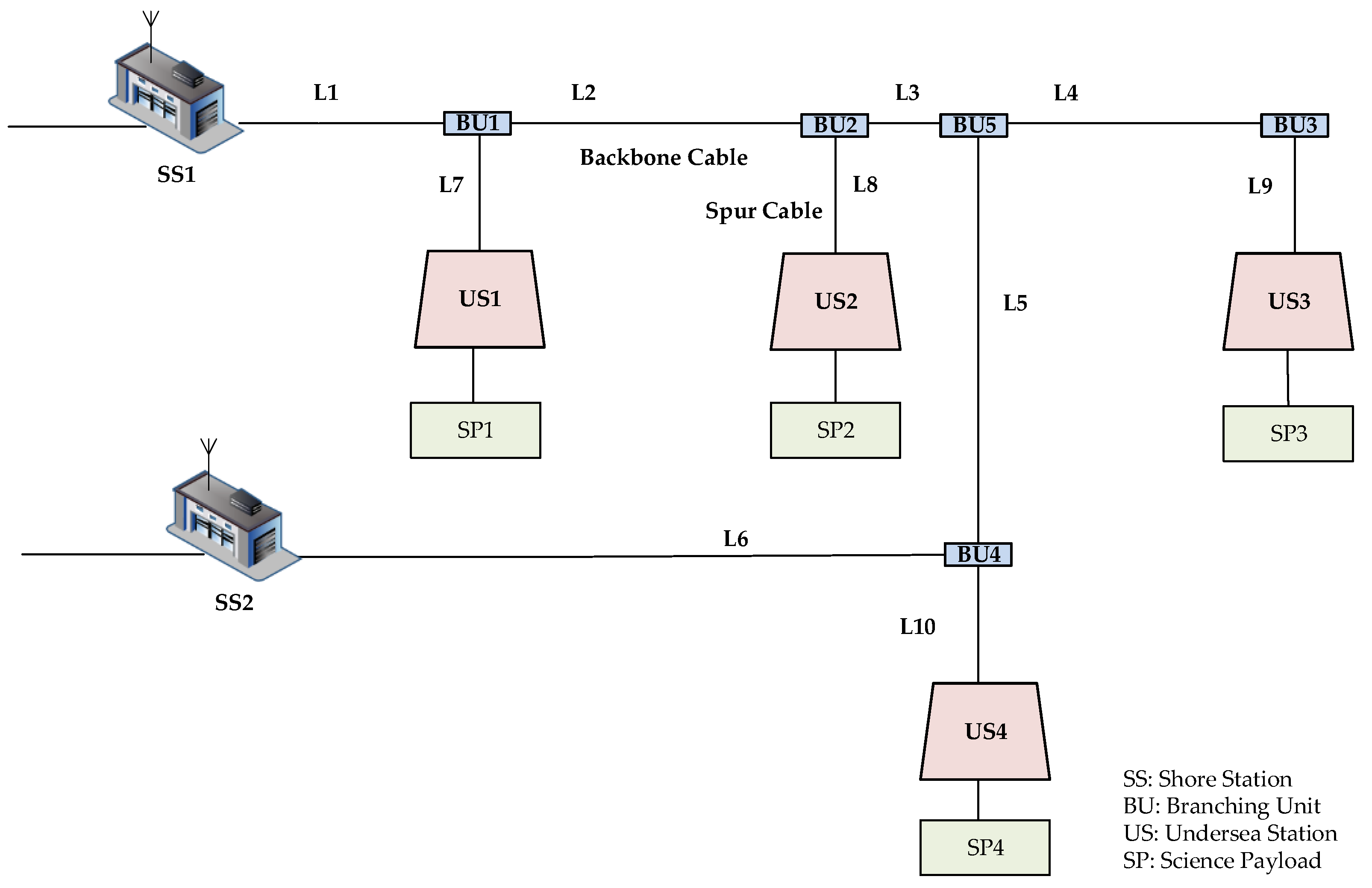
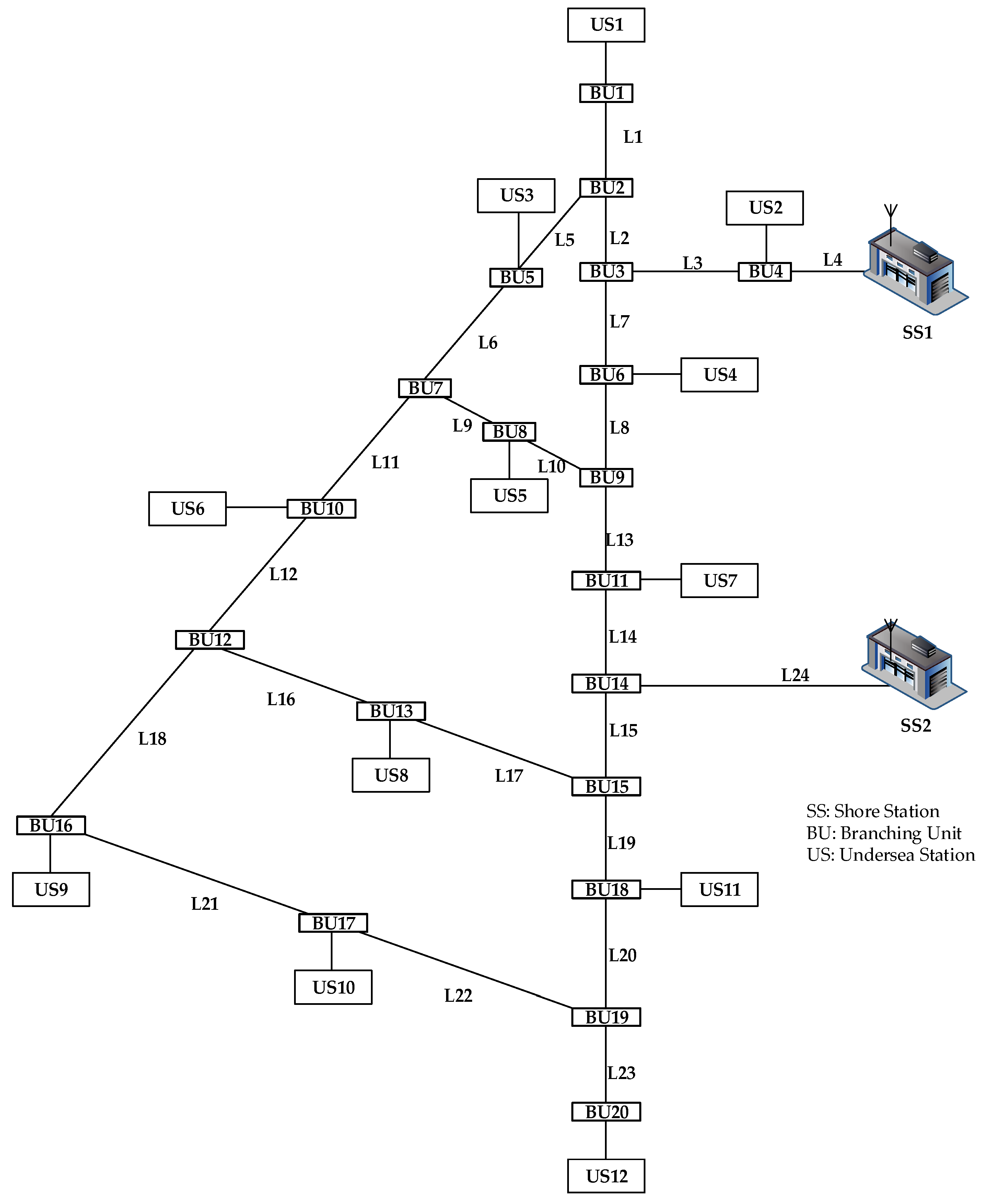
The spur cables are short in length and fixed in position. Their depths and temperatures can be gained through the sensors in the nearest undersea stations, so that the resistances can be calculated through Equation (1) and (2). The voltage of a branch node can be calculated by the spur cable resistance and the input voltage and current of the undersea station. Figure 2 shows a CSO with one shore station and three undersea stations. L1–L3 are the backbone cables, and L4–L6 are the spur cables. The voltage of BU1 can be calculated by the function:

$$V_2=V_5-I_{25}{R}_{25}$$

(3)

where $R_{25}$ means the spur cable resistance between BU1 and US1.

The backbone cables have much wider seafloor distribution than the spur cables. In summer, the shallow seawater temperature can be up to 30 °C, but the deep-sea seawater temperature is only 2–4 °C. As the backbone cable resistances are various, parameter estimation is used to improve the power system model accuracy.

The cable resistances and the undersea stations’ voltage and current values have a linear relation, e.g., in Figure 2,

$$V_1=I_{12}{R}_{L1}+I_{25}{R}_{25}+V_5$$

(4)

where $R_{L1}$ means the unknown resistance of backbone cable L1. Other values can be obtained by measurements or Formula (3).

Selecting 15 measurements as a set of data, we used the least squares method for parameter estimation to obtain the resistances of backbone cables [13].

The branch node voltage calculated in this step is not accurate. In order to ensure the accuracy of fault location, state estimation was used to improve the branch node data accuracy and to prepare for the fault location in the next step.

2.3. State Estimation of Key Nodes

For a power system of CSOs, the state data of branch nodes is essential for system state evaluation, system topology analysis, and fault location. The system state is estimated using the redundancy of real-time data to improve data accuracy and eliminate the error information caused by random noise [14,15].

In CSOs, only the input voltages and currents of undersea stations and the output voltages and currents of shore stations are available. This information can be used to build the power system measurement equation, which is expressed as:

$$z=h\left(x\right)+\nu$$

(5)

where z means measurement vector, x means unknown state data, ν represents the measurement error vector, and h(x) represents the relationship between the unknown state data and the measurement data. For a CSO with a specific topology, the relationship between the measured sensor data and the unknown state data can be obtained by Kirchhoff’s law.

Given the measurement vector z, it is difficult to find an x that makes the residual error zero. Therefore, we hope that x can minimize the sum of squares of the weighted residual. At this point, the state estimation vector x should satisfy the following objective function:

$$\mathrm{J}\left(\mathrm{x}\right)={\left[\mathrm{z}-h\left(\mathrm{x}\right)\right]}^T{R}^{-1}\left[\mathrm{z}-h\left(\mathrm{x}\right)\right]={\displaystyle \sum }_{i=1}^n{\left(r_i/{\sigma }_i\right)}^2\to \min$$

(6)

where R⁻¹ represents the weight, which is a diagonal matrix whose diagonal element is ${\sigma }_i{}^2$, and $\sigma$ means the standard deviation of measurements. Usually, 15 consecutive measurements are used to calculate the standard deviation.

The essential state estimation method can reduce the influence of a large number of small measurement errors. However, the sensors of CSOs generate gross errors sometimes. In the power system, there are some leverage points, which may affect the state estimation results. In order to reduce the influence of gross errors and leverage points, a robust state estimation method is applied to calculate the unknown quantities and to reduce the influence of large measurement errors in the process of state estimation, using a weight factor to control the weights of different residuals [16]. We use k₀ and k₁ to be the critical values. When a measurement residual is smaller than the critical value k₀, this measurement is considered to be trusted and its weight factor is 1; when a measurement residual is greater than k₀ and smaller than the critical value k₁, its weight factor is evaluated between (0,1); when a measurement residual is greater than the critical value k₁, it is considered to be an error and its weight factor is 0.

The voltage and current measurements can be regarded as normal distributions. The probabilities of measurement errors greater than 1.5σ and 2σ is 0.13 and 0.046, respectively. In the process of data pre-processing, when a sample’s gross error is greater than 2.41σ, it is considered to be an error and should be removed. Considering the data pre-processing and the normal distribution, we set the critical value of k₀ to be 1.5σ, and k₁ to be 2σ. The weight factor can be expressed as:

$${\omega }_i=\{\begin{array}{c} 1, \left|v_i\right|\le 1.5\sigma \hfill \\ \frac{1.5}{\left|v_i\right|}, 1.5\sigma <\left|v_i\right|\hfill \\ 0, 2\sigma \le \left|v_i\right|\hfill \end{array}<2\sigma$$

(7)

The extremal function can be expressed as:

$${\rho }_i=\{\begin{array}{c}\frac{1}{2}{v}_i^2 , \left|v_i\right|\le 1.5\\ 1.5\left|v_i\right|-0.5{\left(1.5\right)}^2, 1.5<\left|v_i\right|<2\\ a, \left|v_i\right|>2\end{array}$$

(8)

The objective function can be expressed as:

$$J\left(x\right)={\displaystyle \sum }_{i=1}^n{\rho }_i$$

(9)

where v_i represents the residuals of the data and a is a constant and independent of residuals.

According to Equation (5) and Kirchhoff’s law, the state estimation equations of a CSO power system can be established. The objective function of the robust state estimation can be established by Equation (9). The iterative calculation of Formula (5) is carried out until the objective function is satisfied. Then, the state data of the key nodes can be obtained.

2.4. Topology Identification Based on State Estimation

During steady state with no internal disturbances, the variation of measurement data indicates that the power system produces abnormalities and may have faults. Thus, it is necessary to determine whether the data variation represents failure in the CSO, and set relevant thresholds. Thresholds are usually set empirically.

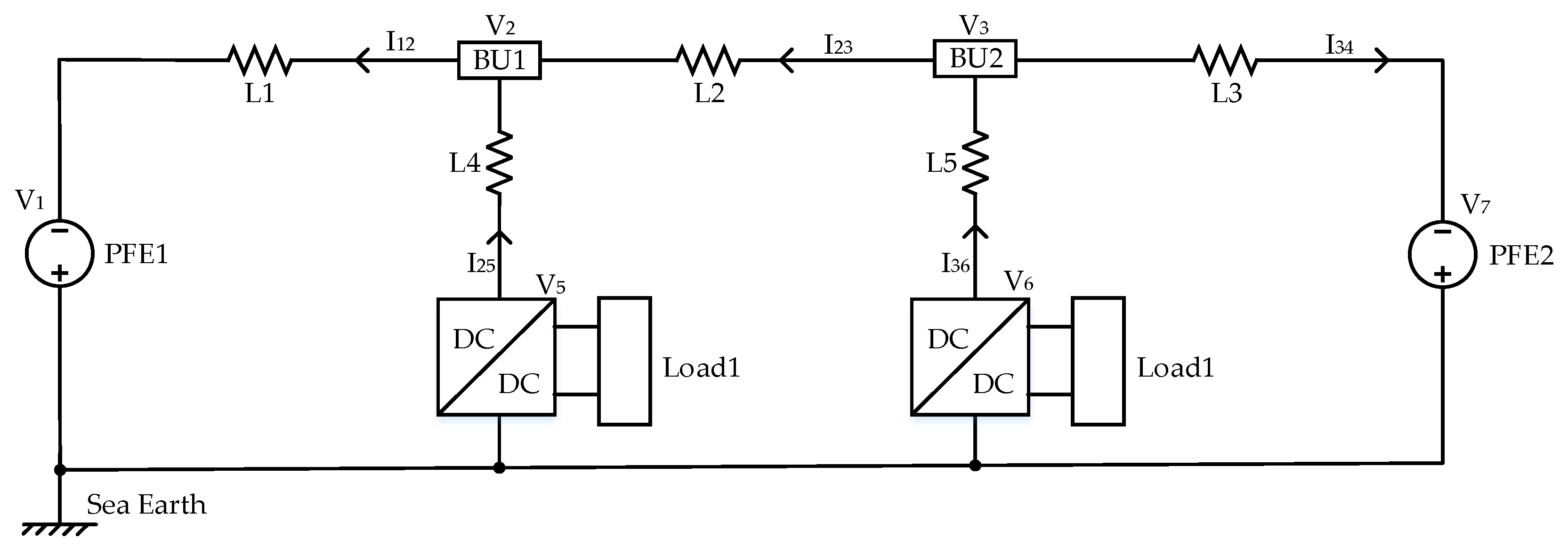
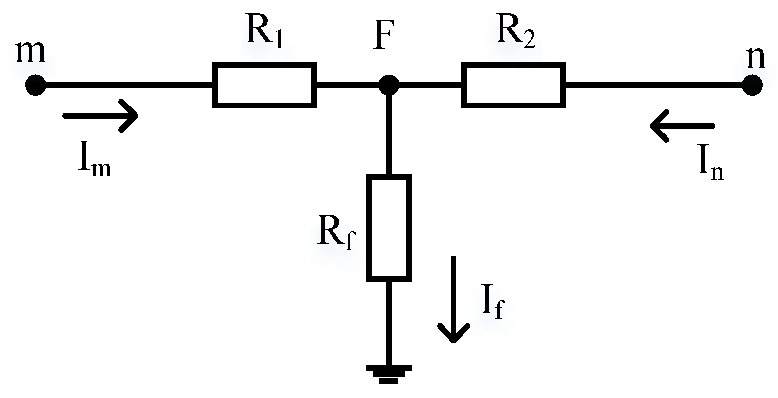
A CSO is segmented by the BUs. If there is a fault, each cable segment will be assumed to have a fault successively. As shown in Figure 3, the current from the left of the fault is expressed by I_m, and the current from the right of the fault is expressed by I_n. According to the measurements and the state estimation, we can judge whether the segment has a cable fault.

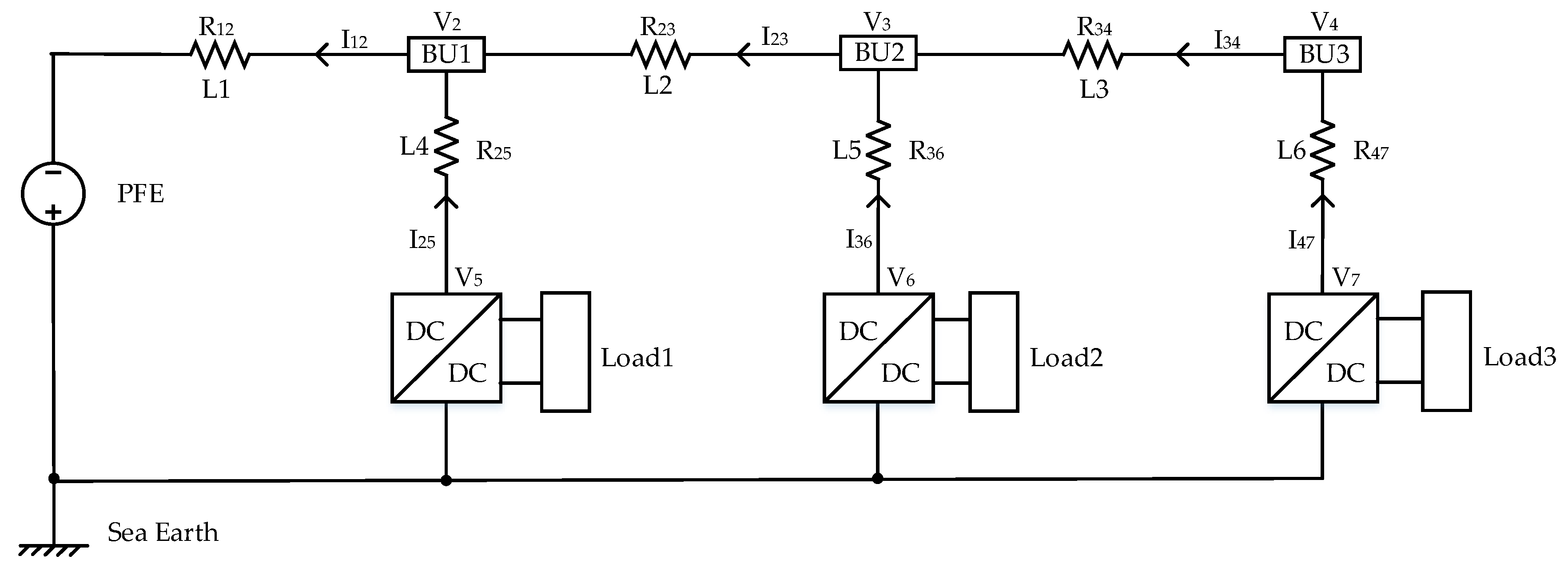
Using the structure shown in Figure 2 as an example, the submarine cable between BU1 and BU2 is assumed to have a sea ground fault.

The measurements include the output voltage V₁ and current I₁₂ of the shore station, the input voltages V₅, V₆, V₇ and currents I₂₅, I₃₆, I₄₇ of the three undersea stations. The voltages V₂, V₃, and V₄ at the BUs cannot be measured directly. When no fault occurs, the cable current between BU_i-1 and BU_i can be expressed as $\frac{v_i-v_{i+1}}{R_i}$. Thus, we use a judgment factor η to determine whether the cable between the nodes i and i + 1 has a fault:

$$\eta =\raisebox{1ex}{$\left(\frac{v_i-v_{i+1}}{R_i}-I_n\right)$}\!\left/ \!\raisebox{-1ex}{$\left(I_m-I_n\right)$}\right.$$

(10)

where I_m represents the current from the left of the fault and I_n represents the current from the right of the fault. For the CSO in Figure 2, using Kirchhoff’s law and the known quantities I₁₂, I₂₅, I₃₆, and I₄₇, the unknown quantities I_m and I_n can be calculated.

If the assumed fault cable segment was on the left of the actual fault one, e.g., between SS and BU1, then i = 1, and Formula (10) is used to calculate η. As a matter of fact, this cable segment does not break down, so that $\frac{v_1-v_2}{R_{12}}=I_m$. and $\frac{v_1-v_2}{R_{12}}\ne I_n$, and the result is η = 1. When the assumed fault cable segment was on the right the actual fault one, e.g., between BU2 and BU3, and i = 3, the result is $\frac{v_3-v_4}{R_{34}}=I_n,$ so that η = 0. When the assumed fault cable segment was the actual one, the result is 0 < η < 1, and the fault location can be calculated.

We can suppose the fault occurred on each cable segment in turn, and calculate η. When 0 < η < 1, it is considered that this cable segment has a fault, and then the new topology of the CSO considering the fault can be obtained.

2.5. Fault location Identification

The power system topology of a CSO is renewed when locating the fault section. In Figure 3, m and n are two BUs; F is the fault point; R₁ and R₂ are the cable impedances; I_m and I_n are currents from BU_m to the fault point and BU_n to fault point, respectively; R_f and I_f are the grounding impedance and the grounding current of the fault point respectively; R_mn is the impedance between m and n. The relationships among them are as follows:

$$U_m=R_1{I}_m+R_f{I}_f$$

(11)

$$I_f=I_m+I_n$$

(12)

$$R_1=M{R}_{mn}$$

(13)

$$R_2=\left(1-M\right)R_{mn}$$

(14)

According to Equations (11) and (14), the fault impedance R_f and the parameter M can be obtained. If the distance between BU_m and BU_n is L, the distance from the fault point to the BU_m is M·L.

3. Simulation Results

3.1. Component Models

3.1.1. Submarine Cable Model

In order to verify the feasibility of the method, we carried out a simulation experiment on CSO models. Voltage drops, caused by the cable resistances, the repeaters and the BUs, are important parameters to determine the fault location.

A short cable segment can be modelled by a π circuit, including a resistor, an inductor, and two capacitors. Figure 4 shows the circuit model of long submarine cables. Under steady state, the effect of cable inductance and capacitance can be neglected. The typical CSO cable resistance is 1 Ω/km in 20 °C.

3.1.2. BU Model

The voltage drops along the power transmission line are important parameters to calculate the fault location. In addition to the voltage drops caused by the submarine cables, the BUs also produce voltage drops [5]. The schematic diagram of a BU is shown in Figure 5.

In Figure 5, the d1, d2, d3 and d4 represent zener diodes, which are used to power relay switching circuits. Two pairs of bidirectional diodes are designed for bidirectional backbone currents. The voltage drop of one BU is:

$$V_{BU}=2\times V_{ZenerReverse}+2\times V_{ZenerForward}$$

(15)

where V_ZenerReverse = 6.9 V and V_ZenerForward = 0.7 V.

3.1.3. DC/DC Converter Model

The DC/DC converters in undersea stations are used to step down the HVDC from the transmission line, and the schematic diagram of DC/DC converters is shown in Figure 6. In the laboratory prototype, the output power range of the DC/DC converter is 20 W to 200 W. The conversion efficiency is calculated by measuring the input power and output power of the converter, and the results are shown in Figure 7. The conversion efficiency can be approximated as quadratic polynomials. Using state estimation to locate the fault point, the conversion efficiency of the DC/DC converters are taken into account in this paper:

$$V_{out}{I}_{out}=V_{in}{I}_{in}·n$$

(16)

where $V_{out}$ and $I_{out}$ are the state data in U₀ side and $V_{in}$ and $I_{in}$ are the state data in U side; the conversion efficiency is n. $V_{in}$ can be regarded as an unknown quantity, and Equation (16) can be added to the state estimation to improve data redundancy and thus improve the accuracy of state estimation.

3.2. Constraint Condition

In this paper, we focuse on the high resistance fault location. Therefore, the topologies of CSOs, fault locations, and other factors will affect the value range of fault resistance, e.g., in Figure 2, if there is a fault in L1, the fault resistance R_f can be expressed as:

$$R_f=\frac{V_1-I_{m}m{R}_{12}}{I_R}$$

(17)

where:

$$m=\frac{\raisebox{1ex}{$(V_1-V_2)$}\!\left/ \!\raisebox{-1ex}{$R_{12}-I_n$}\right.}{I_m-I_n}$$

(18)

$$I_m=I_{12}$$

(19)

$$I_n=I_{25}+I_{36}+I_{47}$$

(20)

$$I_R=I_m-I_n$$

(21)

$$V_2=V_5-I_{25}\times R_{25}$$

(22)

$$I_{25}=\frac{P_1}{V_5\times n}$$

(23)

$$I_{36}=\frac{P_2}{V_6\times n}$$

(24)

$$I_{47}=\frac{P_3}{V_7\times n}$$

(25)

In these equations, the DC/DC conversion efficiency is n, and the load power consumptions of undersea stations are P₁, P₂, and P₃. The minimum startup voltage of undersea stations is 50% of the output voltage of the PFE in the shore station. Thus, the high resistance fault must meet the following conditions:

$$\{\begin{array}{c}{V}_5>0.5V_1\\ V_6>0.5V_1\\ V_7>0.5V_1\end{array}$$

(26)

3.3. Simulation Results

Typical topologies of CSOs are the chained structure with one power supply [17,18], the annular structure with two-terminal power supplies [19,20], and the meshed structure [21,22]. In this part, we use SABER to set up the model, get the state data, and give the data the error of 1% artificially. Then, we use MATLAB to implement the fault location algorithm. The proposed fault location method is simulated and verified under different topologies. The influence of fault locations, fault resistances, and load powers on fault location accuracies is also studied.

3.3.1. Chained Structure with One Power Supply

Figure 2 shows a CSO with a chained structure with one power supply, a shore-based station connected with one backbone cable, and the undersea stations that have no redundant power transmission line. Typical representatives are MARS (Monterey Accelerated Research System) [18,23], OOI (Ocean Observatory Initiative) [17], VRNUS (Victoria Experimental Network Under the Sea) [24], and East China Sea Experimental Seafloor Observatory [25].

According to the topology of Figure 2, we set the length of each backbone cable L1, L2, and L3 as 100 km, the length of each spur cable L4, L5, and L6 as 10 km, the load power Load1, Load2, and Load3 as 50 W, and the output voltage of the shore station as 400 V. Simulation experiments verify the effects of different fault segments, fault resistances and fault distances. The results are shown in

Table 1. Fault location accuracies in a chained structure.

Fault Cable Segments	Fault Distances (km)	Fault Resistances (Ω)	Fault Location Errors (km)
L1	30	2000	0.14
		3000	0.47
		4000	0.22
	50	2000	0.41
		3000	0.51
		4000	0.59
	70	2000	0.31
		3000	0.67
		4000	0.52
L2	130	2000	0.20
		3000	0.17
		4000	0.21
	150	2000	0.14
		3000	0.32
		4000	0.01
	170	2000	0.11
		3000	0.393
		4000	0.44
L3	220	2000	0.04
		3000	0.26
		4000	0.71
	250	2000	0.18
		3000	0.65
		4000	0.23
	270	2000	0.17
		3000	0.67
		4000	0.87

. The fault can be located by the proposed approach, and the fault location errors can be kept at less than 1 km under these experiments.

In order to further prove the applicability and robustness of the proposed fault location method, the fault location accuracy has been verified in different load powers, and the results are shown in

Table 2. The effect of loads on fault location accuracies in a chained structure.

Load (W)	Fault Resistances (Ω)	Fault Cable Segments	Fault Location Errors (km)
125	4000	L2	0.17
150	4000	L2	0.38
175	4000	L2	0.96

. In the simulation, the total load of three undersea stations is set to 125 W, 150 W, or 175 W. When the total load is 125 W, the load of US1 is 25 W, and both US2 and US3 are 50 W. When the total load is 150 W, the load of each load is 50 W. When the total load is 175 W, the load of US1 is 75 W, and both US2 and US3 are 50 W. We can see that the fault location errors can also be kept at less than 1 km under these experiments.

3.3.2. Annular Structure with Two-Terminal Power Supplies

In the annular structure with two-terminal power supplies, when a fault occurs and the fault cable is isolated, the CSO is divided into two chained structures. NEPTUNE (North-East Pacific Time-Series Underwater Networked Experiment) in Canada [19] and DONET (Dense Ocean-floor Network System for Earthquakes and Tsunamis) in Japan [20] are annular structures.

Figure 8 is a typical topology diagram of annular structure, which consists of two shore stations and two undersea stations. The output voltage of each shore station is 400 V. The lengths of backbone cables L1, L2, and L3 are 100 km, 50 km, and 50 km respectively. The lengths of spur cables L4 and L5 are 10 km. Each undersea station’s load is 100 W.

In this topology, a fault is set with different fault segments, fault resistances, and fault distances, and the results are shown in

Table 3. Fault location accuracies in an annular structure.

Fault Cable Segments	Fault Distances (km)	Fault Resistances (Ω)	Fault Location Errors (km)
L1	20	1000	0.16
		2000	0.33
		3000	0.21
	50	1000	0.48
		2000	0.03
		3000	0.73
	80	1000	0.07
		2000	0.41
		3000	0.30
L2	110	1000	0.04
		2000	0.15
		3000	0.89
	125	1000	0.48
		2000	0.03
		3000	0.73
	140	1000	0.73
		2000	0.68
		3000	0.59
L3	170	1000	0.09
		2000	0.82
		3000	0.10
	175	1000	0.53
		2000	0.07
		3000	0.14
	185	1000	0.94
		2000	0.15
		3000	0.47

. Moreover,

Table 4. The effect of loads on fault location accuracies in an annular structure.

Load (W)	Fault Resistances (Ω)	Fault Cable Segments	Fault Location Errors (km)
400	4000	L2	0.26
300	4000	L2	0.34
200	4000	L2	0.85

shows the fault location accuracy is verified in different load powers. It can be seen from the results that the fault location accuracies are within 1 km in the annular structure in these experiments.

3.3.3. Meshed Structure

Figure 9 shows a schematic diagram of a meshed structure, which is a simplified topology of the NEPTUNE project in the early stage [5,21,22]. This meshed structure consists of two shore stations, 12 undersea stations and 20 BUs. The length of each backbone cable is 100 km and the length of each spur cable is 10 km. The output voltage of each shore station is 10 kV, and the load of each underwater station is 1 kW.

According to the propagation of error, when:

$$N=f\left(x_1,x_2,\dots ,x_n\right)$$

(27)

The relative error of N is:

$$\frac{\Delta N}{N}=\left|\frac{\partial lnf}{\partial x_1}\right|\Delta x_1+\left|\frac{\partial lnf}{\partial x_2}\right|\Delta x_2+\cdots +\left|\frac{\partial lnf}{\partial x_n}\right|\Delta x_n$$

(28)

After calculating the relative error of BUs, the BUs in Figure 9 can be divided into three types. The first type is connect to a spur cable or a shore station directly; the relative error is only associated with the measurement of its connected US, such as BU 1, 4, 5, 6, 8, 10, 11, 13, 14, 16, 17, 18, and 20. The second type is not connect to a spur cable or a shore station, and the relative error is associated with multiple USs, such as BU 3, 7, 9, 12, and 15. The third type’s relative error is associated with the measurement of one US, but they are not connect to a spur cable or a shore station directly, such as BU 1 and 19. Cable segments can be classified according to the type of BU at both ends. We selecte the three most representative segments for the test, which are L6, L21, and L23.

The influence of fault cable segments, fault resistances and fault distances on fault positioning accuracy is shown in

Table 5. Fault location accuracies in a meshed structure.

Fault Cable Segments	Fault Distances (km)	Fault Resistances (Ω)	Fault Location Errors (km)
L6	415	2000	0.45
		3000	0.59
		4000	0.70
	450	2000	0.86
		3000	0.38
		4000	0.19
	485	2000	0.28
		3000	0.17
		4000	0.78
L21	830	2000	0.06
		3000	0.66
		4000	0.45
	850	2000	0.24
		3000	0.72
		4000	0.54
	870	2000	0.21
		3000	0.38
		4000	0.51
L23	930	2000	0.43
		3000	0.66
		4000	0.51
	950	2000	0.19
		3000	0.85
		4000	0.91
	970	2000	0.58
		3000	0.55
		4000	0.86

. The fault location errors are less than 1 km in the experiment.

3.3.4. A Specific Case Study

The topology of a CSO to be built in the East China Sea is shown in Figure 1. This CSO consists of two shore stations, five BUs, and four undersea stations. The output voltage of shore stations SS1 and SS2 are 400 V, and the lengths of backbone cables L1, L2, L3, L4, L5, and L6 are 170 km, 80 km, 10 km, 100 km, 90 km, and 80 km, respectively. The lengths of spur cables L7, L8, L9, and L10 are 10 km. The loads of US1, US2, US3, and US4 are 100 W, 100 W, 50 W, and 150 W, respectively. As mentioned above, we locate the faults with different fault segments, fault resistances, and fault distances. The location results are shown in

Table 6. Fault location accuracies in a Y-type structure.

Fault Cable Segments	Fault Distances (km)	Fault Resistances (Ω)	Fault Location Errors (km)
L1	70	1000	0.64
		1300	0.13
		2100	0.16
	85	1000	0.23
		1300	0.07
		2100	0.56
	100	1000	0.42
		1300	0.11
		2100	0.36
L2	200	1000	0.04
		1300	0.11
		2100	0.35
	210	1000	0.45
		1300	0.32
		2100	0.63
	220	1000	0.45
		1300	0.17
		2100	0.25
L4	300	1000	0.13
		1300	0.59
		2100	0.47
	320	1000	0.44
		1300	0.15
		2100	0.68
	340	1000	0.42
		1300	0.63
		2100	0.54
L5	305	1000	0.09
		1300	0.16
		2100	0.78
	325	1000	0.07
		1300	0.13
		2100	0.47
	340	1000	0.82
		1300	0.65
		2100	0.38
L6	370	1000	0.57
		1300	0.33
		2100	0.67
	390	1000	0.55
		1300	0.36
		2100	0.27
	405	1000	0.28
		1300	0.46
		2100	0.24
L7	175	1500	0.35
L8	255	1500	0.58
L9	365	1500	0.78
L10	355	1500	0.13

. The fault location accuracy is kept within 1 km.

3.4. Laboratory Prototype Experiment Results

According to the topology of the CSO in the East China Sea, a circuit prototype is established in our laboratory, shown in Figure 10. DC power supplies are used to simulate shore stations; the output voltages of the power supplies are 400 V. In this prototype, we use resistors, inductors, and capacitors to simulate the submarine cables. The connection relationship is shown in Figure 4, and the cable resistance is 1 Ω/km.

The effects of fault segments, fault resistances and fault distances on fault location errors are verified in the CSO laboratory prototype.

Table 7. The effect of fault segments on fault location accuracies tested on the laboratory prototype.

Fault Resistances (Ω)	Fault Cable Segments	Errors of Fault Location (km)
1300	L1	0.57
1300	L2	0.36
1300	L4	0.84
1300	L5	0.18
1300	L6	0.11

,

Table 8. The effect of fault resistances on fault location accuracies tested on the laboratory prototype.

Fault Distances (km)	Fault Resistances (Ω)	Errors of Fault Location (km)
200	1300	0.26
200	2100	0.18
320	1300	0.17
320	2100	0.17

and

Table 9. The effect of fault distances on fault location accuracies tested on the laboratory prototype.

Fault Cable Segments	Fault Distances (km)	Errors of Fault Location (km)
L2	200	0.26
L2	220	0.41
L6	390	0.69
L6	410	0.11

show the errors of fault location in different fault segments, fault resistances and fault distances, respectively. The experimental results show that the fault location errors can be kept at less than 1 km under different situations.

In the prototype, the resistance errors of the cable prototypes are set to be about 1%, to simulate the influence of seawater temperature variations on the submarine cable resistances. Parameter estimation is a process of estimating unknown parameters in a population distribution from random samples taken from the population. In this paper, the cable resistance is taken as an unknown parameter, and estimated according to the measured voltage and current values. The fault location results, with or without parameter estimation, are compared, as shown in Figure 11. It can be seen that, when the step of parameter estimation is carried out, the fault positioning accuracy will be higher, and the positioning error is less than 1 km. Otherwise, the fault location error will be larger.

4. Conclusions

CSOs are becoming important tools for oceanography research. A novel on-line cable fault location method is proposed to reduce the repair cost of CSOs caused by submarine backbone and spur cable faults. This method is based on robust state estimation and data pre-processing to reduce the influence of gross errors on fault location accuracies, and using parameter estimation to reduce the influence of seawater temperature variation on cable resistances. In the fault location, we only use state data that collected by sensors in the power system, without additional equipment, so that the system stability can be ensured and the costs can be reduced. The experiment results by the computer simulation and the laboratory prototype show that the positioning error of the method is within 1 km.

References

1. Wang, P.X. Seafloor observatories: The third platform for earth system observation. Chin. J. Nat. 2007, 29, 125–130. [Google Scholar]
2. Dai, J.X.; Liu, J.; Wang, Y.W. Analysis of reason of faults of HV cable and the countermeasures. High Volt. Eng. 2004, 30, 54–56. [Google Scholar]
3. Zhu, Y.H.; Qian, A.I.; Feng, L.U. Survey of power cable fault location. Relay 2006, 34, 81–88. [Google Scholar]
4. Schneider, K.; Liu, C.C.; Howe, B. Topology error identification for the NEPTUNE power system. IEEE Trans. Power Syst. 2005, 20, 1224–1232. [Google Scholar] [CrossRef]
5. Chan, T.; Liu, C.C.; Howe, B.M.; Kirkham, H. Fault location for the NEPTUNE power system. IEEE Trans. Power Syst. 2007, 22, 522–531. [Google Scholar] [CrossRef]
6. Liu, C.C.; Schneider, K.; Kirkham, H.; Howe, B. State estimation for the NEPTUNE power system. In PES Transmission and Distribution Conference and Exposition; IEEE: Dallas, TX, USA, 2003; Volume 2, pp. 748–754. [Google Scholar]
7. Lu, S.; El-Sharkawi, M.A. NEPTUNE Power System: Detection and Location of Switch Malfunctions and High Impedance Faults. In Proceedings of the IEEE International Symposium on Industrial Electronics; IEEE: Montreal, QC, Canada, 2006; Volume 2, pp. 1960–1965. [Google Scholar]
8. Schneider, K.; Liu, C.C.; McGinnis, T.; Howe, B.; Kirkham, H. Real-time Control and Protection of the NEPTUNE Power System; IEEE: Biloxi, MI, USA, 2002; Volume 3, pp. 1799–1805. [Google Scholar]
9. Livani, H.; Evrenosoglu, C.Y. A single-ended fault location method for segmented HVDC transmission line. Electr. Power Syst. Res. 2014, 107, 190–198. [Google Scholar] [CrossRef]
10. Nanayakkara, O.M.K.K.; Rajapakse, A.D.; Wachal, R. Location of DC line faults in conventional HVDC systems with segments of cables and andoverhead lines using terminal measurements. IEEE Trans. Power Deliv. 2012, 27, 279–288. [Google Scholar] [CrossRef]
11. Namdari, F.; Salehi, M. A new algorithm for wide area fault location in power system. In Proceedings of the Power System Conference; IEEE: Tehran, Iran, 2015; pp. 363–370. [Google Scholar]
12. Lin, L.F.; Xiao, H.; Xian-Qiu, W.U. Comparison between Chauvenet’s criterion and Grubbs criterion. Phys. Exp. Coll. 2012, 25, 86–88. [Google Scholar]
13. Golub, G. Numerical methods for solving linear least squares problems. Numer. Math. 1965, 7, 206–216. [Google Scholar] [CrossRef]
14. Monticelli, A. Electric power system state estimation. Proc. IEEE 2000, 88, 262–282. [Google Scholar] [CrossRef]
15. Schweppe, F.C.; Handschin, E.J. Static state estimation in electric power systems. Proc. IEEE 1974, 62, 972–982. [Google Scholar] [CrossRef]
16. Huber, P.J. Robust estimation of a location parameter. Ann. Math. Stat. 1964, 35, 73–101. [Google Scholar] [CrossRef]
17. Cowles, T.; Delaney, J.; Orcutt, J.; Weller, R. The Ocean Observatories Initiative: Sustained ocean observing across a range of spatial scales. Mar. Technol. Soc. J. 2010, 44, 54–64. [Google Scholar] [CrossRef]
18. Massion, G.; Raybould, K. MARS: The Monterey accelerated research system. Sea Technol. 2006, 47, 39–42. [Google Scholar]
19. Barnes, C.R.; Best, M.M.R.; Johnson, F.R.; Pautet, L.; Pirenne, B. Challenges, benefits, and opportunities in installing and operating cabled ocean observatories: Perspectives from NEPTUNE Canada. IEEE J. Ocean. Eng. 2013, 38, 144–157. [Google Scholar] [CrossRef]
20. Kaneda, Y. The advanced ocean floor real time monitoring system for mega thrust earthquakes and tsunamis—Application of DONET and DONET2 data to seismological research and disaster mitigation. In Proceedings of the Oceans; IEEE: Seattle, WA, USA, 2010; pp. 1–6. [Google Scholar]
21. El-Sharkawi, M.A.; Upadhye, A.; Lu, S.; Kirkham, H.; Howe, B.M.; Mcginnis, T.; Lancaster, P. North East Pacific Time-Integrated Undersea Networked Experiments (NEPTUNE): Cable switching and protection. IEEE J. Ocean. Eng. 2005, 30, 232–240. [Google Scholar] [CrossRef]
22. Kirkham, H.; Lancaster, P.; Liu, C.C.; El-Sharkawi, M.; Howe, B.M. The NEPTUNE power system: Design from fundamentals. In Proceedings of the International Workshop on Scientific Use of Submarine Cables & Related Technologies; IEEE: Tokyo, Japan, 2003; pp. 301–306. [Google Scholar]
23. Henthorn, R.G.; Hobson, B.W.; Mcgill, P.R.; Sherman, A.D.; Smith, K.L. MARS Benthic Rover: In-situ rapid proto-testing on the Monterey Accelerated Research System. In Proceedings of the Oceans; IEEE: Seattle, WA, USA, 2010; pp. 1–7. [Google Scholar]
24. Dewey, R.; Round, A.; Macoun, P.; Vervynck, J.; Tunnicliffe, V. The VENUS cabled observatory: Engineering meets science on the seafloor. In Proceedings of the Oceans; IEEE: Vancouver, BC, Canada, 2007; pp. 398–404. [Google Scholar]
25. Lyu, F.; Zhou, H. Progress of scientific cabled seafloor observatory networks. J. Eng. Stud. 2016, 8, 139–154. [Google Scholar]
Figure 1. A typical CSO structure planned to be applied in the East China Sea.
Jmse 08 00190 g001
Figure 2. The power system diagram of a chained structure CSO.
Jmse 08 00190 g002
Figure 3. Schematic diagram of a cable fault.
Jmse 08 00190 g003
Figure 4. The circuit model of long submarine cables.
Jmse 08 00190 g004
Figure 5. The simplified schematic diagram of a BU.
Jmse 08 00190 g005
Figure 6. The schematic diagram of CSO DC/DC converters.
Jmse 08 00190 g006
Figure 7. The conversion efficiency of CSO DC/DC converters.
Jmse 08 00190 g007
Figure 8. The power system diagram of an annular structure CSO.
Jmse 08 00190 g008
Figure 9. The schematic diagram of a meshed structure CSO.
Jmse 08 00190 g009
Figure 10. The CSO laboratory prototype for fault location experiments.
Jmse 08 00190 g010
Figure 11. The fault location results with or without parameter estimation.
Jmse 08 00190 g011