A Vector Sensor-Based Acoustic Characterization System for Marine Renewable Energy


Abstract
1. Introduction
2. Materials and Methods
2.1. Hardware
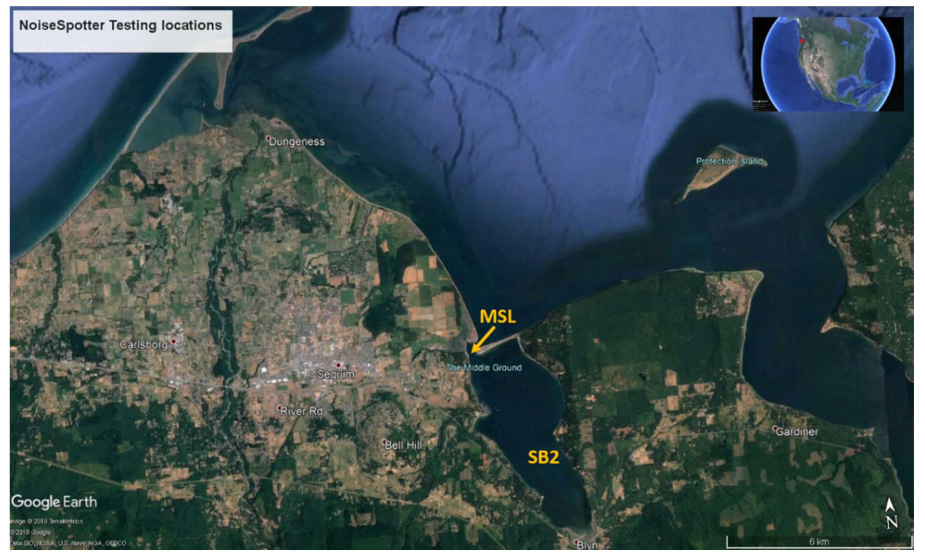
2.2. Field Testing
3. Results
3.1. Data Quality
3.2. Signal to Noise Ratio
3.3. Flow Noise Removal
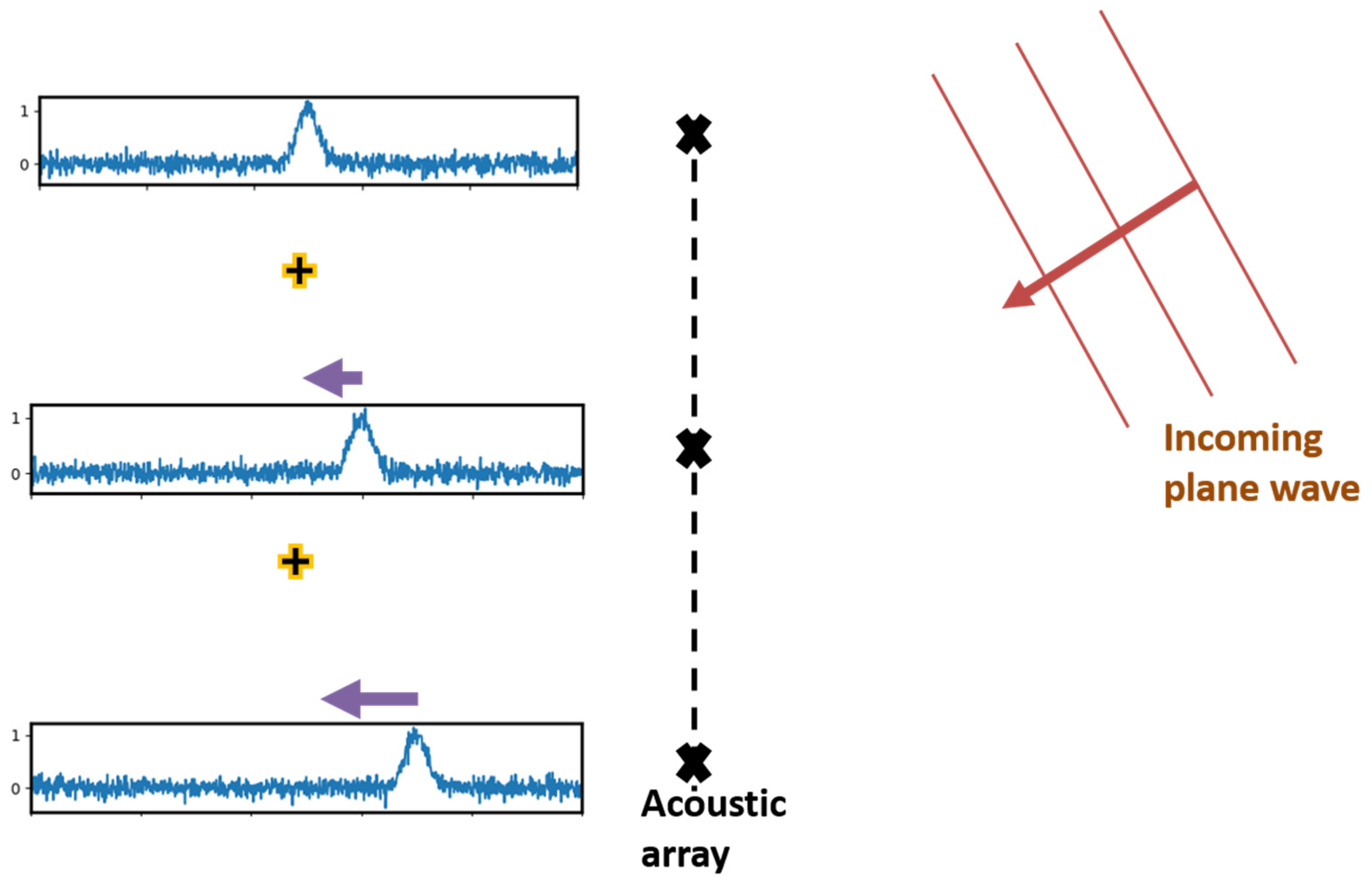
3.4. Location Estimation
4. Discussion and Summary
- Development of a three-dimensional vector sensor array using a modular frame whose acoustic impedance is very close to that of seawater;
- Quantitative characterization of flow noise contamination, and its suppression in an energetic channel, applied to a vector sensor;
- Application of a location estimation algorithm to an in-water acoustic source.
5. Conclusions
Author Contributions
Funding
Acknowledgments
Conflicts of Interest
References
- Copping, A.; Sather, N.; Hanna, L.; Whiting, J.; Zydlewski, G.; Staines, G.; Gill, A.; Hutchison, I.; O’Hagan, A.; Simas, T.; et al. Annex IV 2016 State of the Science Report: Environmental Effects of Marine Renewable Energy Development Around the World. Ocean Energy Syst. 2016, 224. [Google Scholar]
- Roche, R.C.; Walker-Springett, K.; Robins, P.E.; Jones, J.; Veneruso, G.; Whitton, T.A.; Piano, M.; Ward, S.L.; Duce, C.E.; Waggitt, J.J.; et al. Research priorities for assessing potential impacts of emerging marine renewable energy technologies: Insights from developments in Wales (UK). Renew. Energy 2016, 99, 1327–1341. [Google Scholar] [CrossRef]
- National Marine Fisheries Service. 2018 Revisions to: Technical Guidance for Assessing the Effects of Anthropogenic Sound on Marine Mammal Hearing (Version 2.0): Underwater Thresholds for Onset of Permanent and Temporary Threshold Shifts; NOAA Technical Memorandum NMFS-OPR-59; US Department of Commerce, NOAA: Silver Spring, MD, USA, 2018; p. 167.
- Haxel, J.; Turpin, A.; Matsumoto, H.; Klinck, H. A portable, real-time passive acoustic system and autonomous hydrophone array for noise monitoring of offshore wave energy projects. In Proceedings of the Marine Energy Technology Symposium, Washington, DC, USA, 25 April 2016. [Google Scholar]
- Greene, C.R., Jr.; McLennan, M.W.; Norman, R.G.; McDonald, T.L.; Jakubczak, R.S.; Richardson, W.J. Directional frequency and recording (DIFAR) sensors in seafloor recorders to locate calling bowhead whales during their fall migration. J. Acoust. Soc. Am. 2004, 116, 799–813. [Google Scholar] [CrossRef] [PubMed]
- Rush, B.; Stewart, A.; Joslin, J.; Polagye, B. Development of an adaptable monitoring package for marine renewable energy projects Part 1: Conceptual design and operation. In Proceedings of the 2nd Marine Energy Technology Symposium, Global Marine Renewable Energy Conference, Seattle, WA, USA, 18 April 2014. [Google Scholar]
- Chandrayadula, T.; Miller, C.W.; Joseph, J. Monterey Bay ambient noise profiles using underwater gliders. Proc. Meet. Acoust. 2013, 19, 070031. [Google Scholar]
- Polagye, B.; Noe, J.; Crisp, C.; Cotter, E.; Murphy, P. Drifting Acoustic Instrumentation for Marine Energy, Poster. In Proceedings of the International Conference on the Environmental Interactions of Marine Energy Technologies, Orkney, UK, 24–27 April 2018. [Google Scholar]
- D’Spain, G.L.; Hodgkiss, W.S.; Edmonds, G.L. The simultaneous measurement of infrasonic acoustic particle velocity and acoustic pressure in the ocean by freely drifting Swallow floats. IEEE J. Ocean. Eng. 1991, 16, 195–207. [Google Scholar] [CrossRef]
- Thode, A.; D’Spain, G.L.; Kuperman, W.A. Matched-field processing, geoacoustic inversion, and source signature recovery of blue whale vocalizations. J. Acoust. Soc. Am. 2000, 107, 1286–1300. [Google Scholar] [CrossRef] [PubMed]
- Tougaard, J. Underwater noise from a wave energy converter is unlikely to affect marine mammals. PLoS ONE 2015, 10. [Google Scholar] [CrossRef]
- Hawkins, A.D.; Popper, A.N. Assessing the impact of underwater sound on fishes and other forms of marine life. Acoust. Today 2014, 10, 30–41. [Google Scholar]
- NDT Resource Center. Available online: https://www.nde-ed.org/GeneralResources/MaterialProperties/UT/ut_matlprop_index.htm (accessed on 14 February 2020).
- Mellinger, D.K.; Stafford, K.M.; Moore, S.E.; Dziak, R.P.; Matsumoto, H. An overview of fixed passive acoustic observation methods for cetaceans. Oceanography 2007, 20, 36–45. [Google Scholar] [CrossRef]
- McKenna, M.; Wiggins, S.M.; Hildebrand, J.A. Underwater radiated noise from modern commercial ships. J. Acoust. Soc. Am. 2012, 92, 92–103. [Google Scholar] [CrossRef]
- Bassett, C.; Thomson, J.; Dahl, P. Flow noise and turbulence in two tidal channels. J. Acoust. Soc. Am. 2014, 135, 1764–1774. [Google Scholar] [CrossRef] [PubMed]
- D’Spain, G.L. Energetics of the Deep Ocean’s Infrasonic Sound Field. Ph.D. Thesis, University of California, San Diego, CA, USA, 1990. [Google Scholar]
- Thode, A.; Skinner, J.; Scott, P.; Roswell, J. Tracking sperm whales with a towed acoustic sensor. J. Acoust. Soc. Am. 2010, 128, 2681–2694. [Google Scholar] [CrossRef] [PubMed]
- Nehorai, A.; Paldi, E. Acoustic vector sensor array processing. J. Acoust. Soc. Am. 1994, 51, 1479–1491. [Google Scholar] [CrossRef]
- Santos, P.; Felisberto, P.; Hursky, P. Source localization with vector sensor array during the Makai experiment. In Proceedings of the 2nd International Conference and Exhibition on “Underwater Acoustic Measurements: Technologies and Results”, Heraklion, Greece, 25–29 June 2007; pp. 895–900. [Google Scholar]
- Merchant, N.; Brookes, K.; Faulkner, R.; Bicknell, A.W.J.; Godley, B.J.; Witt, M.J. Underwater noise levels in UK waters. Sci. Rep. 2016, 6, 36942. [Google Scholar] [CrossRef]
- Hester, K.C.; Peltzer, E.T.; Kirkwood, W.J.; Brewer, P.G. Unanticipated consequences of ocean acidification: A noisier ocean at lower pH. Geophys. Res. Lett. 2008, 35, L19601. [Google Scholar] [CrossRef]
- National Research Council. Ocean Noise and Marine Mammals; The National Academies Press: Washington, DC, USA, 2003. [Google Scholar]
- The Global Ocean Observing System. Available online: https://www.goosocean.org/index.php?option=com_content&view=article&id=14&Itemid=114 (accessed on 14 February 2020).
- OSPAR Commission. Available online: https://www.ospar.org/ (accessed on 14 February 2020).
- Joint Monitoring Program for Ambient Noise North Sea. Available online: https://northsearegion.eu/jomopans/ (accessed on 14 February 2020).
- Nedelec, S.L.; Campbell, J.; Radford, A.N.; Simpson, S.D.; Merchant, N.D. Particle motion: The missing link in underwater acoustic ecology. Methods Ecol. Evol. 2016, 7, 836–842. [Google Scholar] [CrossRef]
- Holler, R.A. The Evolution of the Sonobuoy from World War II to the Cold War; No. JUA-2014-025-N; NAVMAR APPLIED SCIENCES CORP: Warminster, PA, USA, 2014. [Google Scholar]
- McDonald, M.A. DIFAR hydrophone usage in whale research. Can. Acoust. 2004, 32, 155–160. [Google Scholar]
- Kaplan, M.; Mooney, T. Coral reef soundscapes may not be detectable far from the reef. Sci. Rep. 2016, 6, 31862. [Google Scholar] [CrossRef]
- Horodysky, A.Z.; Brill, R.W.; Fine, M.L.; Musick, J.A.; Latour, R.L. Acoustic pressure and particle motion thresholds in six sciaenid fishes. J. Exp. Biol. 2008, 211, 1504–1511. [Google Scholar] [CrossRef]
- McConnell, J.A. Analysis of a compliantly suspended acoustic velocity sensor. J. Acoust. Soc. Am. 2003, 113, 1395. [Google Scholar] [CrossRef] [PubMed]
- Brienzo, R.K.; Hodgkiss, W.S. Broadband matched-field processing. J. Acoust. Soc. Am. 1993, 94, 2821–2831. [Google Scholar] [CrossRef]


© 2020 by the authors. Licensee MDPI, Basel, Switzerland. This article is an open access article distributed under the terms and conditions of the Creative Commons Attribution (CC BY) license (http://creativecommons.org/licenses/by/4.0/).
Share and Cite
Raghukumar, K.; Chang, G.; Spada, F.; Jones, C. A Vector Sensor-Based Acoustic Characterization System for Marine Renewable Energy. J. Mar. Sci. Eng. 2020, 8, 187. https://doi.org/10.3390/jmse8030187
Raghukumar K, Chang G, Spada F, Jones C. A Vector Sensor-Based Acoustic Characterization System for Marine Renewable Energy. Journal of Marine Science and Engineering. 2020; 8(3):187. https://doi.org/10.3390/jmse8030187
Chicago/Turabian StyleRaghukumar, Kaustubha, Grace Chang, Frank Spada, and Craig Jones. 2020. "A Vector Sensor-Based Acoustic Characterization System for Marine Renewable Energy" Journal of Marine Science and Engineering 8, no. 3: 187. https://doi.org/10.3390/jmse8030187
APA StyleRaghukumar, K., Chang, G., Spada, F., & Jones, C. (2020). A Vector Sensor-Based Acoustic Characterization System for Marine Renewable Energy. Journal of Marine Science and Engineering, 8(3), 187. https://doi.org/10.3390/jmse8030187