Article

Extraction Method of Offshore Mariculture Area under Weak Signal based on Multisource Feature Fusion

1
College of Geomatics, Shandong University of Science and Technology, Qingdao 266590, China
2
Marine Physics and Remote Sensing Research Department, First Institute of Oceanography, Ministry of Natural Resources, Qingdao 266061, China
*
Author to whom correspondence should be addressed.
J. Mar. Sci. Eng. 2020, 8(2), 99; https://doi.org/10.3390/jmse8020099
Submission received: 7 January 2020 / Revised: 28 January 2020 / Accepted: 3 February 2020 / Published: 6 February 2020

Abstract

:
Mariculture is crucial in environmental monitoring and safety assurance of marine environments. Certain mariculture areas are often partially or completely submerged in water, which causes the target signal to be extremely weak and difficult to detect. A method of target recognition and classification based on the convolutional neural network called semantic segmentation can fully consider the space spectrum and context semantic information. Therefore, this study proposes a target extraction method on the basis of multisource feature fusion, such as nNDWI and G/R ratio. In this work, the proposed recognition algorithm is verified under the conditions of uniform distribution of strong, weak, and extremely weak signals. Results show that the G/R feature is superior under the condition of uniform distribution of strong and weak signals. Its mean pixels accuracy is 2.32% higher than RGB (combination of red band, green band, and blue band), and its overall classification accuracy is 98.84%. Under the condition of extremely weak signal, the MPA of the multisource feature method based on the combination of G/R and nNDWI is 10.76% higher than RGB, and the overall classification accuracy is 82.02%. Under this condition, the G/R features highlight the target, and nNDWI suppresses noise. The proposed method can effectively extract the information of weak signal in the marine culture area and provide technical support for marine environmental monitoring and marine safety assurance.

1. Introduction

Offshore mariculture has had a growing impact on offshore marine environments in recent years, due to the continuous development of the offshore mariculture industry. This type of mariculture may cause serious underlying dangers to offshore marine safety, especially in cultivation areas, which are submerged in water and difficult to find. Therefore, on-time monitoring and identifying the coastal mariculture area under weak signal is important in safety assurance and engineering construction of marine environments. Earth observation technology of remote sensing has the advantages of wide coverage, strong timeliness, and low cost, which provide an effective means for the identification of mariculture areas.
At present, the target recognition and classification methods of remote sensing images can be divided into traditional statistical methods [1,2,3,4,5,6,7,8], machine learning methods [9,10,11], and deep learning algorithms [12,13,14]. The traditional statistical methods realize the classification by using statistical analysis of the gray value and texture of image. However, this method has low classification accuracy and serious noise. In comparison with traditional statistical methods, the classification algorithms based on machine learning (fuzzy cluster analysis, expert system classification, support vector machine, decision tree classification, and object-oriented image classification) can improve classification accuracy to a certain extent, but establishing complex functions is difficult due to the limitation of machine learning network structures, which are unsuitable for high-resolution remote sensing images with complex spatial features. Moreover, machine learning networks have poor generalization ability. Deep learning is a new algorithm developed in the field of machine learning. The algorithms are mainly divided into three network structures in the field of image classification, namely, stacked autoencoders (SAE), deep belief network (DBN), and convolutional neural networks (CNN). SAE and DBN can only input one-dimensional characteristic data because of its limitation in network structure. At present, CNN is a widely used classification algorithm because it can fully extract the deep information of images and process complex samples. However, for features with very high spatial resolution and large differences in intraclass and small differences with interclass, several salt-and-pepper noises often exist in the classification results on the basis of the traditional deep CNN. Semantic segmentation algorithms based on deep CNN are trained using the end-to-end method to realize the classification of remote sensing objects. Semantic segmentation can consider not only the spectral and spatial characteristics but also extract context information. At present, many semantic segmentation networks have emerged, such as FCN [15], DeepLabv3 [16,17], PSPNet [18], U-Net [19], SegNet [20], and RefineNet [21]. Among these networks, the DeepLabv3 algorithm using the structure of MultiGrid and parallel modules with atrous convolution (ASPP) has the best performance in the VOC2012 dataset, and the precision of mean intersection over union reaches 86.9. However, the above methods have not been applied to the identification and extraction of offshore mariculture areas under weak signals.
Antinormalized difference water index (nNDWI) is an antiwater index that can weaken the signal of seawater. The G/R band is a kind of data that can stretch and normalize the specific region of the ratio of green band to red band. Meanwhile, the red band has strong absorption in water to ensure that the G/R band features can highlight the difference between water and nonwater objects. As such, this study proposes a DeepLabv3 semantic segmentation method with multisource feature for extracting mariculture area under weak signal. This method exploits the features provided by the nNDWI and G/R ratio band to complete the target recognition and classification under weak signal.

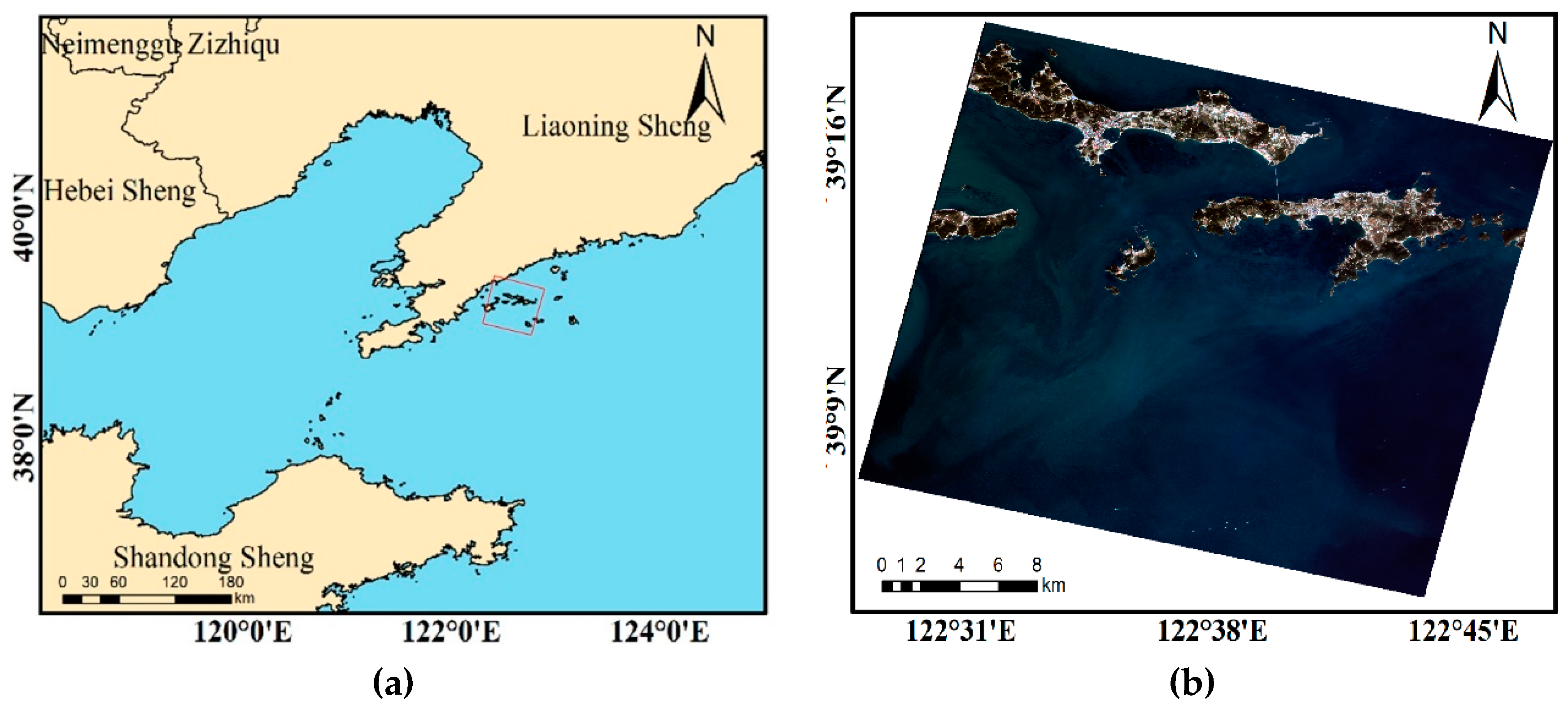
2. Research Area and Data Source

In this study, the experimental area is located in the midlatitude sea area around Changhai County, Dalian City, Liaoning Province, China with a longitude between 122°28.08′E and 122°47.34′E and a latitude between 39°4.21′N and 39°18.93′N as shown in Figure 1. The warm, temperate, semihumid monsoon climate with four distinct seasons of Changhai County is warm in the winter and cool in summer. The annual average temperature is 10 °C, and the average temperature in summer is 25 °C. Such climate is suitable for fishery development. Changhai County is a large mariculture county in China. Its fishery accounts for more than 80% of the total agricultural economy, and the sea area reaches 200 km2. In the offshore mariculture area of Changhai County, the majority of the mariculture are semisubmerged. Therefore, the weak characteristic signal of the mariculture area in the image data causes certain difficulties and obstacles in extracting offshore mariculture.
This study works on a GF-2 remote sensing image. GF-2 is a sun synchronous orbit satellite with an orbit inclination of 97°54.48′ and a local time of 10:30 AM at the satellite landing point. The spatial resolution of the image is 3.24 and 0.81 m for multispectral and panchromatic images, respectively. The imaging time of the data used in this study is 19 September 2017, and the band settings are presented in Table 1.

3. Method

The proposed semantic segmentation method based on multisource feature fusion includes three parts, namely, band combination, data preprocessing, and model training. The specific process is shown in Figure 2.

3.1. Band Feature Combination

The band features used in this study are B, G, R, nNDWI, and G/R. Near-infrared band (NIR) demonstrates strong absorption in water, whereas nNDWI can highlight nonwater signals. Therefore, nNDWI was used instead of the NIR band and is defined as follows:
nNDWI = 1 − NDWI = 1 − (G − NIR)/(G + NIR),
G/R can highlight the difference between obstacles and seawater background. Hence, this study also chose G/R as the main band feature.
G/R = G/R,

3.2. Preprocessing

3.2.1. Image Fusion

First, the multispectral and panchromatic images taken by GF-2 were orthographically corrected. Given that most of the images were offshore, the altitude was set to 0. The multispectral and panchromatic images were then fused to obtain high-resolution multispectral data.

3.2.2. Data Stretching and Normalization

For bands B, G, and R, the DN(Digital Number) value was divided by 1024 to adjust the data distribution between 0 and 1. For nNDWI and G/R ratios, we normalized them by Equations (3) and (4), respectively.
nNDWI = nNDWI / max ( nNDWI ) ,
G / R = { 0 ( G / R < 1.5 ) G / R 1.5 2 ( 1.5 G / R 3.5 ) 1 ( G / R > 1.5 ) ,

3.2.3. Image Cutting

The display memory limitation of GPU and the large spatial pixel scale of remote sensing image prevents the direct placement of the entire image into the network. Cutting the image into small patch images and feeding them into the network in an orderly manner is an effective solution. In this study, by considering the network field of vision and the memory consumption during training, the original image was cut into small images with a width and height of 600 pixels for training, and the total memory consumption during training was controlled at around 14.3 GB. The starting coordinates of the cut image were randomly selected in Equation (5).
{(x, y) | 0 ≤ x ≤ (width ‒ 600), 0 ≤ y ≤ (height ‒ 600)},

3.2.4. Data Augmentation

To enhance the generalization and accuracy of the training model, this study expanded the number of samples in the original training dataset by rotating, mirroring, and adding Gaussian noise.
(1)
Rotation
(2)
In remote sensing imaging, the shooting angles of the objects are different, and all objects present different states in the image. Therefore, the image is randomly rotated by 0°, 90°, 180°, and 270° after cutting to expand the sample dataset.
(3)
Mirroring
(4)
In order to expand the training sample, we will randomly mirror the image horizontally, vertically, or in both directions.
(5)
Adding Gaussian noise.
The atmosphere and other factors will lead to slightly different images of the same objects. In this study, the generalization of the final model was enhanced by increasing the Gaussian noise to expand the training samples under different imaging conditions. The mean value of the Gaussian noise used in the experiment is 0 and the standard deviation is 1.

3.3. Model Training

The network used in this study is the DeepLabv3 semantic segmentation network, and its structure is shown in the following Figure 3.
In the first half of DeepLabv3, ResNet-v2-50, which contains four blocks (Table 2), was used to extract image features. The basic unit of each block is the residual structure, as shown in Figure 4. The gradient dispersion problem of deep network in the training process can be effectively alleviated through this residual structure. At the same time, numerous batch normalization layers were used to prevent the gradient explosion caused by the wide distribution of feature data. The second half of DeepLabv3 used the atrous spatial pyramid pooling (ASPP) layer to obtain the feature data of multiscale. The ASPP layer uses the expansion convolution of different expansion coefficients to obtain the feature of large view field with small-scale convolution kernel. Finally, the feature map of multiscale view field was obtained by superposing the feature map of different scales of view fields.
In this experiment, the Geospatial Data Abstraction Library image library was used to read multiband image data and save the segmented image generated via prediction. The model generated by network training was saved in the form of check point. To obtain the optimal model on the training set, the model saving strategy used in this paper is presented as follows:
(1)
Define the variable loss-A and its initial value before network training. The initial value used in this experiment was 1.8.
(2)
After 20 rounds of training, calculate the average loss-b of the 20 rounds of training (loss-B).
(3)
From the 20 rounds of training data, 25% of the data were randomly selected as a temporary test set. Calculate the error of network to temporary test set (loss-C).
(4)
If both loss-C and loss-B are less than loss-A, save the model and change the value of loss-A to loss-C. If the appeal conditions are not tenable, no change will be made.
(5)
After another 20 rounds of training, return to step 2.

4. Results and Discussion

4.1. Environment Parameter Setting

To improve the training speed, the network uses GPU for training under the Linux operating system. The specific software and hardware environments and training parameters are listed in Table 3.

4.2. Experiment Setup

On the basis of the processed data, four groups of band combinations are carried out in this study, and the settings of band combinations are presented in Table 4.
By taking the first group as the control group and comparing it with the three other groups, we can assess the effect of G/R ratio and nNDWI on the network prediction results.
In this experiment, the evaluation indicators of network prediction results are mean pixel accuracy (MPA), overall image accuracy (OA), and the Kappa coefficient. Their calculation method is shown in Equations (6)–(8). The k in the equation refers to the number of classes. The N in the equation is the total number of pixels. P i j refers to the probability that j-type targets are classified as i-type targets. X i j refers to the number of pixels of type j target classified as type i target. X i + refers to the number of real pixels of type i. X + i refers to the number of pixels classified as type i.
M P A = 1 k + 1 i = 0 k p i i j = 0 k p i j ,
O A = 1 N i = 1 k x i i ,
K a p p a = N i = 1 k x i i i = 1 k x i + × x + i N 2 i = 1 k x i + × x + i ,

4.3. Results

Under the influence of hardware acceleration, the training time of the four experimental groups was almost the same, about 10 h.
To reduce the influence of missing data of image edge on the prediction results, the adjacent images in the test set will have 10 overlapping pixels when the cut image is patched. When the classification results of the patched images are combined, five pixels will be taken from both sides for overlap splicing. To show the performance and stability of the network trained by each group under different signal conditions, the experimental results are divided into two parts. The first part is the test of target classification accuracy under the condition of uniform distribution of strong and weak signals. The second part is the test of target classification accuracy under the condition of extremely weak signal. To display the information in the original image clearly, this study shows the original image via RMS stretching.

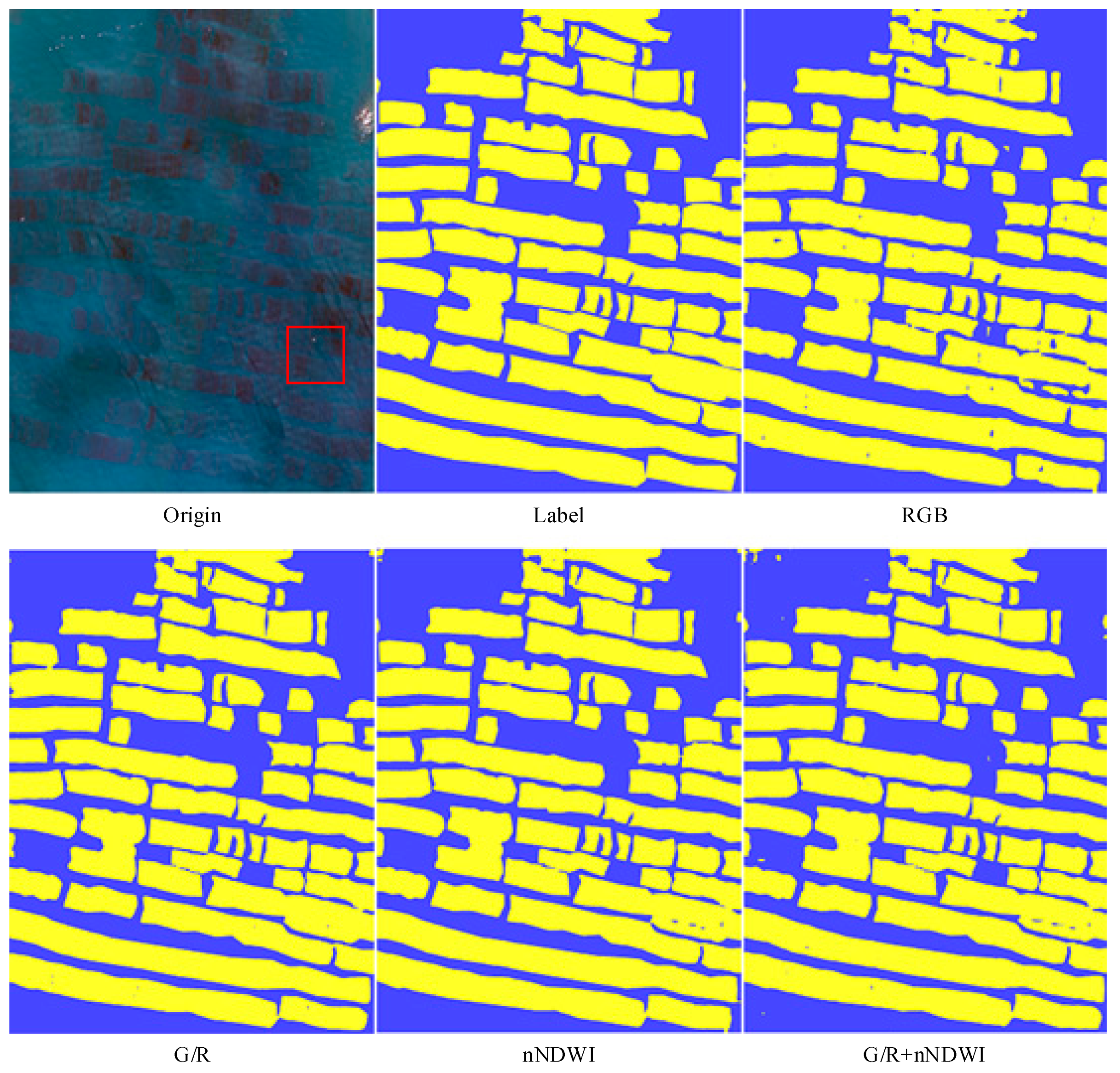
4.3.1. Results under Uniform Distribution of Strong and Weak Signals

In this study, an 1485 × 1974 area was selected for testing, and the testing area was entirely and partially evaluated. The classification results are presented in Figure 5.
The recognition accuracy of each group is generally higher under the condition of uniform distribution of strong and weak signals. However, the second, third, and fourth groups significantly improved in contrast with the first group. The RGB band features are clearly misclassified, and additional small debris exist in the identified obstacles. This phenomenon is rarely seen in the three other groups of classification results. Among them, G/R has the least debris phenomenon and the best performance.
The enlarged display of the classification results in the red box in Figure 5 is shown in Figure 6. The first group has evident misclassification phenomenon and is unstable. The three other groups don’t or rarely show this phenomenon.
From the evaluation indicators of the classification results shown in Table 5, the evaluation indicators of the latter three groups are significantly higher than those of the first group. The second group is the most prominent under the condition of uniform distribution of strong and weak signals. MPA is 2.32% higher than the original RGB, and OA increased by 2.22%. In addition, the Kappa coefficient is increased by 0.0447.

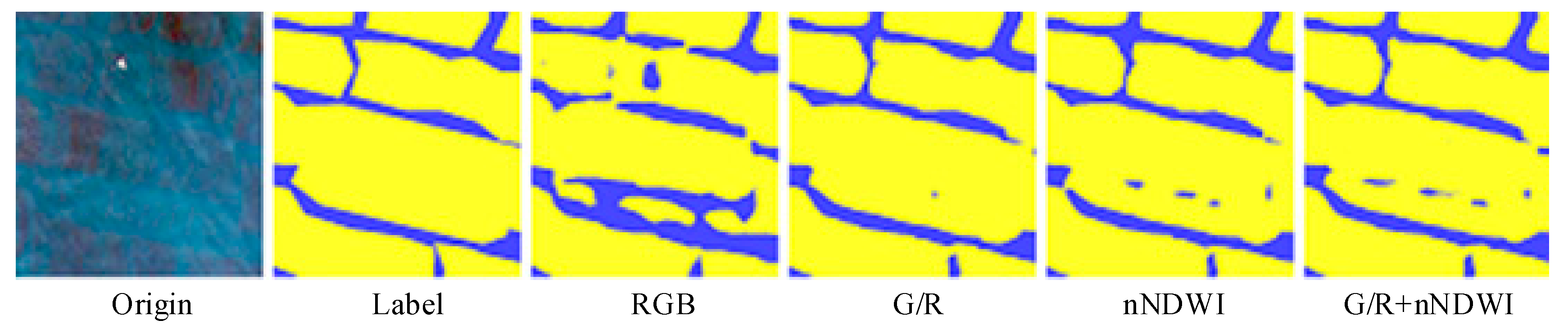
4.3.2. Results under Extremely Weak Signal

Under the condition of uniform distribution of strong and weak signals, each group has high accuracy in weak signal recognition. However, they may recognize the weak signal information between the strong signals by analyzing the semantic information of strong signals. When no strong signal exists in the scene, the performance of the network may fluctuate remarkably. Therefore, the second test is carried out under the condition of extremely weak signal. The classification results and evaluation accuracy are presented in Figure 7.
The overall effect is significantly weaker than that under the condition of uniform distribution of strong and weak signals due to the extreme test environment. However, in Figure 7, the effect of the second and fourth groups is significantly better than that of the first and third groups. The first group mistakenly identified almost all the backgrounds as targets. The third group failed to recognize most of the targets. However, the accuracy of the third group is higher than that of the first and second groups.
Figure 8 is an enlarged view of the classification results in the red box of Figure 7. Although the effect of the third and fourth groups is relatively good—from the local point of view shown in Figure 8—these groups are still affected by the noise and incorrectly recognize the background between the targets as the targets. The fourth group improves the accuracy of classification by combining the features of the third and second groups to suppress noise and reduce the wrong pixels. This finding shows that the fourth group of network has good stability in performance.
From the evaluation indicators of the classification results shown in Table 6, under the condition of extremely weak signal, the fourth group inherits not only the higher classification accuracy of the second group but also combines the recognition accuracy of the third group to the target to improve classification accuracy in general. The MPA of the fourth group is 10.76% higher than that of the original RGB, and OA increased by 16.51%. The Kappa coefficient increased by 0.34. Under the condition of extremely weak signal, the fourth group has satisfactory classification performance.
Results show that the G/R ratio and nNDWI features have certain advantages in the recognition of weak signal targets in offshore mariculture areas. Under the condition of uniform distribution of strong and weak signals, the classification effect of RGB, G/R ratio, and nNDWI is almost the same. In comparison with the traditional RGB data, under the condition of extremely weak signal, the recognition effect of the G/R ratio and nNDWI features is significantly better. The combination of G/R ratio and nNDWI can improve the stability of the network performance in the unstable recognition environment.
Finally, SVM (support vector machine) is compared with DeepLabv3. We use RGB band combination to compare their classification accuracy under the condition of uniform distribution of strong signal and weak signal. The classification results are as follows:
As can be seen from Figure 9, the classification performance of SVM is weaker than the method proposed in this paper. In the prediction results of SVM, the targets with weak signals are difficult to identify and some of the targets with dense intersection are fuzzy.
From the evaluation results in Table 7, Deeplabv3 is obviously superior to SVM in all evaluation indexes. Compared with SVM, the MPA, OA, and Kappa coefficients of Deeplabv3 are 20.03%, 20.48%, and 0.43 higher, respectively.

5. Conclusions

This study presents a method of target extraction in weak signal environments. By using the DeepLabv3 semantic segmentation method on the basis of multisource features, such as nNDWI and G/R ratio, the target recognition and classification of mariculture areas in weak signal environments are realized. The following conclusions can be drawn from this study:
1)
Under the condition of uniform distribution of strong and weak signals, the G/R characteristic is superior. The semantic segmentation method based on this feature demonstrated that MPA is 2.32% higher than the RGB band feature, and OA is higher by 2.22%. In addition, the Kappa coefficient is higher by 0.04%, and the overall classification accuracy is 98.84%.
2)
Under the condition of extremely weak signal, the multisource feature method MPA based on the combination of G/R and nNDWI is 10.76% higher than RGB, and OA is 16.51% higher. Moreover, the Kappa coefficient is 0.34% higher, and the overall classification accuracy is 82.02%. Under the condition of extremely weak signal, the G/R features highlight the target, and nNDWI suppresses the noise.
3)
The DeepLabv3 semantic segmentation method based on the multisource features of nNDWI and G/R ratio is an effective method for extracting the information of weak signal marine culture areas. It provides technical support for environmental monitoring and safety assurance of marine environments.
At present, the methods in this paper still have some limitations. The best stretching range of G/R ratio is empirical value, which changes with the change of signal environment. This makes the network performance unstable. Moreover, the training of the network requires that the number of strong and weak signal samples are similar, and the location distribution is uniform. The next step is to improve the calculation method of G/R ratio so that it can adapt to the local signal environment and eliminate or reduce the dependence of G/R ratio on the empirical value. Through this improvement, the performance and stability of the network are further improved.

Author Contributions

Conceptualization, C.L. and T.J.; methodology, C.L. and Z.Z.; software, C.L.; validation, B.S., X.P. and Z.Z.; formal analysis, T.J.; investigation, X.P.; resources, Z.Z.; data curation, B.S.; writing—original draft preparation, C.L.; writing—review and editing, T.J.; visualization, B.S.; supervision, X.P.; project administration, L.Z.; funding acquisition, L.Z. and J.Z. All authors have read and agreed to the published version of the manuscript.

Funding

This research was funded by the National Key Research and Development Program of China, grant number 2016YFC1402701; National Natural Science Foundation of China, grant number 41801385; Natural Science Foundation of Shandong Province, grant number ZR2018BD004 & ZR2019QD010; Key Technology Research and Development Program of Shandong, grant number 2019GGX101049.

Conflicts of Interest

The authors declare no conflict of interest.

References

  1. McCauley, S.; Goetz, S.J. Mapping residential density patterns using multi-temporal Landsat data and a decision-tree classifier. Int. J. Remote Sens 2004, 25, 1077–1094. [Google Scholar] [CrossRef]
  2. Wang, H.; Suh, J.W.; Das, S.R. Hippocampus segmentation using a stable maximum likelihood classifier ensemble algorithm. In Proceedings of the 8th IEEE International Symposium on Biomedical Imaging: From Nano to Macro, Chicago, IL, USA, 30 March–2 April 2011. [Google Scholar]
  3. Shahrokh Esfahani, M.; Knight, J.; Zollanvari, A. Classifier design given an uncertainty class of feature distributions via regularized maximum likelihood and the incorporation of biological pathway knowledge in steady-state phenotype classification. Pattern Recognit. 2013, 46, 2783–2797. [Google Scholar] [CrossRef] [PubMed] [Green Version]
  4. Toth, D.; Aach, T. Improved minimum distance classification with Gaussian outlier detection for industrial inspection. In Proceedings of the 11th International Conference on Image Analysis and Processing, Palermo, Italy, 26–28 September 2001. [Google Scholar]
  5. Liu, Z. Minimum distance texture classification of SAR images in contourlet domain. In Proceedings of the International Conference on Computer Science and Software Engineering, Hubei, China, 12–14 December 2008. [Google Scholar]
  6. Fletcher, N.D.; Evans, A.N. Minimum distance texture classification of SAR images using wavelet packets. In Proceedings of the IEEE International Geoscience and Remote Sensing Symposium, Toronto, ON, Canada, 24–28 June 2002. [Google Scholar]
  7. Belloni, C.; Aouf, N.; Caillec, J.L.; Merlet, T. Comparison of Descriptors for SAR ATR. In Proceedings of the 2019 IEEE Radar Conference (RadarConf), Merlet, Boston, MA, USA, 22–26 April 2019; pp. 1–6. [Google Scholar]
  8. Kechagias-Stamatis, O.; Aouf, N.; Nam, D. Multi-Modal Automatic Target Recognition for Anti-Ship Missiles with Imaging Infrared Capabilities. In Proceedings of the IEEE Sensor Signal Processing for Defence Conference (SSPD), London, UK, 6–7 December 2017. [Google Scholar]
  9. Rumelhart, D.E.; Hintont, G.E.; Williams, R.J. Learning representations by back-propagating errors. Nature 2004, 323, 533–536. [Google Scholar] [CrossRef]
  10. Sezer, O.B.; Ozbayoglu, A.M.; Dogdu, E. An artificial neural network-based stock trading system using technical analysis and Big Data Framework. In Proceedings of the SouthEast Conference, Kennesaw, GA, USA, 13–15 April 2017. [Google Scholar]
  11. Smola, A.J.; Schölkopf, B. On a Kernel-Based Method for Pattern Recognition, Regression, Approximation, and Operator Inversion. Algorithmica 1998, 22, 211–231. [Google Scholar] [CrossRef]
  12. Hinton, G.E. Reducing the Dimensionality of Data with Neural Networks. Science 2006, 313, 504–507. [Google Scholar] [CrossRef] [PubMed] [Green Version]
  13. Lecun, Y.; Bottou, L.; Bengio, Y. Gradient-based learning applied to document recognition. Proc. IEEE 1998, 86, 2278–2324. [Google Scholar] [CrossRef] [Green Version]
  14. Kechagias-Stamatis, O.; Aouf, N. Fusing deep learning and sparse coding for SAR ATR. IEEE Trans. Aerosp. Electron. Syst. 2018, 55, 785–797. [Google Scholar] [CrossRef] [Green Version]
  15. Long, J.; Shelhamer, E.; Darrell, T. Fully Convolutional Networks for Semantic Segmentation. IEEE Trans. Pattern Anal. 2014, 39, 640–651. [Google Scholar]
  16. Chen, L.C.; Papandreou, G.; Schroff, F. Rethinking Atrous Convolution for Semantic Image Segmentation. arXiv 2017, arXiv:1706.05587. [Google Scholar]
  17. Zhang, Z.; Huang, J.; Jiang, T. Semantic segmentation of very high-resolution remote sensing image based on multiple band combinations and patchwise scene analysis. JARS 2020, 14, 01620. [Google Scholar] [CrossRef]
  18. Zhao, H.; Shi, J.; Qi, X. Pyramid Scene Parsing Network. In Proceedings of the IEEE Conference on Computer Vision and Pattern Recognition, Honolulu, HI, USA, 21–26 July 2017. [Google Scholar]
  19. Ronneberger, O.; Fischer, P.; Brox, T. U-Net: Convolutional Networks for Biomedical Image Segmentation. MICCAI 2015, 234–241. [Google Scholar] [CrossRef] [Green Version]
  20. Badrinarayanan, V.; Kendall, A.; Cipolla, R. SegNet: A Deep Convolutional Encoder-Decoder Architecture for Image Segmentation. IEEE Trans. Pattern Anal. 2017, 39, 2481–2495. [Google Scholar] [CrossRef] [PubMed]
  21. Lin, G.; Milan, A.; Shen, C. RefineNet: Multi-path Refinement Networks for High-Resolution Semantic Segmentation. In Proceedings of the IEEE Conference on Computer Vision and Pattern Recognition, CVPR, Honolulu, HI, USA, 21–26 July 2017. [Google Scholar]
Figure 1. Study area and GF-2 image. (a) Study area. (b) GF-2 image.
Jmse 08 00099 g001
Figure 2. Experimental flowchart of this study used.
Jmse 08 00099 g002
Figure 3. DeepLabv3 network structure diagram used in this study.
Jmse 08 00099 g003
Figure 4. Residual block structure used in this study.
Jmse 08 00099 g004
Figure 5. Classification results of different band characteristics under uniform distribution of strong and weak signals.
Jmse 08 00099 g005
Figure 6. Comparison of the results of characteristic local classes in the different wavebands.
Jmse 08 00099 g006
Figure 7. Classification results of different groups under extremely weak signal.
Jmse 08 00099 g007
Figure 8. Comparison of noise interference in different groups.
Jmse 08 00099 g008
Figure 9. Comparison of classification accuracy between Deeplabv3 and SVM.
Jmse 08 00099 g009
Table 1. Original data band settings.
Way of ImagingPush Broom Scanning Imaging Mode
SensorPanchromatic bandMultispectral
Resolution0.81 m3.24 m
Wavelength450–900 nmBlue: 450–520 nm
Green: 520–590 nm
Red: 630–690 nm
NIR: 770–900 nm
Table 2. Residual network block structure.
Layer Name50-layer
Conv17 × 7, 64, stride2
3 × 3 max pool, stride2
Block1 [ 1 × 1 , 64 3 × 3 , 64 1 × 1 , 256 ] × 3
Block2 [ 1 × 1 , 128 3 × 3 , 128 1 × 1 , 512 ] × 4
Block3 [ 1 × 1 , 256 3 × 3 , 256 1 × 1 , 1024 ] × 6
Block4 [ 1 × 1 , 512 3 × 3 , 512 1 × 1 , 2048 ] × 3
Table 3. Network operation environment and training parameters.
Running EnvironmentTraining Parameters
Hardware EnvironmentSoftware EnvironmentImage_Size600
CPUi9-9900kOperating systemCentos7Classes2
Learning_rate1e-4
Batch_norm_epsion1e-5
Batch_norm_decay0.9997
GPUP100Programming language and deep learning libraryPython3.7
Tensorflow1.14
Resnet_modelresnet_v2_50
Output_stride16
Batch_size8
Epoches25000
Table 4. Band combinations.
GroupGroup 1Group 2Group 3Group 4
Band combinationR, G, BG/RnNDWIG/R, nNDWI
Table 5. Classification accuracy of different groups under uniform distribution of strong and weak signals.
Parameter NameGroup 1Group 2Group 3Group 4
Background0.94480.98150.9844 10.9813
Target0.98410.9938 10.98990.9882
MPA0.96450.9877 10.98720.9848
OA0.96620.9884 10.98750.9852
Kappa0.93170.9764 10.97460.9699
Time10 h 32 min10 h 13 min10 h 7 min10 h 26 min
1 The bold numbers are the best results of corresponding evaluation indexes
Table 6. Classification accuracy of different groups under extremely weak signal.
Parameter NameGroup 1Group 2Group 3Group 4
Background0.89470.92440.54700.9624 1
Target0.60040.74360.8067 10.7479
MPA0.74750.83400.67690.8551 1
OA0.65510.80730.58770.8202 1
Kappa0.30290.61260.18460.6385 1
Time10 h 32 min10 h 13 min10 h 7 min10 h 26 min
1 The bold numbers are the best results of corresponding evaluation indexes
Table 7. Classification accuracy of RGB bands by Deeplabv3 and SVM.
Parameter NameDeeplabv3SVM
Background0.9448 10.7747
Target0.9841 10.7538
MPA0.9645 10.7642
OA0.9662 10.7614
Kappa0.9317 10.5064
1 The bold numbers are the best results of corresponding evaluation indexes

