Article

Model of Bio-Colonisation on Mooring Lines: Updating Strategy Based on a Static Qualifying Sea State for Floating Wind Turbines

by
Benjamin Decurey
1,*,†,
Franck Schoefs
1,2,
Anne-Laure Barillé
3 and
Thomas Soulard
2,4
1
Institut de Recherche en Génie Civil et Mécanique (GeM)—UMR CNRS 6183, Ecole Centrale de Nantes et Université de Nantes, 44322 Nantes, France
2
Institut Universitaire Mer et Littoral (IUML)—FR CNRS 3473, Université de Nantes, 44322 Nantes, France
3
BIO-LITTORAL, 2 Rue du Château de l’Eraudière, Immeuble Le Nevada, CS 80693, 44306 Nantes CEDEX 3, France
4
Laboratoire de recherche en Hydrodynamique, Énergétique et Environnement Atmosphérique (LHEEA)—UMR CNRS 6598, Ecole Centrale de Nantes, 44321 Nantes, France
*
Author to whom correspondence should be addressed.
Current address: Département de Physique, Université de Nantes—UFR Sciences et Techniques, 2 Chemin de la Houssinière, 44322 Nantes, France.
J. Mar. Sci. Eng. 2020, 8(2), 108; https://doi.org/10.3390/jmse8020108
Submission received: 10 January 2020 / Revised: 29 January 2020 / Accepted: 30 January 2020 / Published: 11 February 2020
(This article belongs to the Special Issue Monitoring of Coastal and Offshore Structures)

Abstract

:
Bio-colonisation affects the ageing of materials and the behaviour of offshore structures. Mooring systems and umbilicals belong to the family of slender bodies which are components sensitive to bio-colonisation because of a change of dynamic behaviour due to shape, roughness and mass modifications. However, this stochastic process in time and space is hard to predict. The purpose is then twofold: first, to provide a stochastic spatial model of the bio-colonisation on a mooring line; second, to show that in some defined environmental conditions, such as low wave height, low wind and current velocities, the monitoring of mooring lines tension can help to assess and reduce uncertainty on this model. Therefore, a comprehensive stochastic modelling based on mussels colonisation was carried out using on-site videotapes, experimental campaigns and expert knowledge. We studied the efficiency of a virtual sensing network using this model and a conditional entropy metric. It is first shown that the spatial model fits well with experimental data, and second that a denser medium accuracy sensor network is to be preferred to a single high accuracy fairlead sensor to reduce the uncertainty on the model parameters. It is then worth updating bio-colonisation on mooring lines during the life-time of a floating wind turbine.

1. Introduction

Depending on the floater’s type, the mooring system’s main function is stationkeeping and/or stability of the floating wind turbine during its entire lifetime: 25 years or more. However, from commissioning, and even before, to decommissioning, sources and factors of premature failure are numerous. Nevertheless, Fontaine et al. [1], in an industry survey, showed that almost half of their surveyed failure events were associated with fatigue and corrosion degradations, thus advising for a better “management of mooring integrity” in this regard.
The lifetime consumed during limited events in time, such as impacts and storms, cannot be accurately predicted. In an offshore context, where operations are expensive and the cost of safety factors is high, one of today’s challenges in mooring lines is to develop preventive methods [2,3] to reduce prior uncertainties on the lifetime consumed by everyday action of waves, current, wind and bio-colonisation to estimate mooring line’s state before a storm for example. However, because of the latter actions’ high variability in time and space, deterministic models fail in accurately predicting their state. Monitoring is, therefore, a valuable option to update preferred probabilistic models. This paper aims to reduce prior uncertainties on one of these actions’ main parameters- bio-colonisation mass, through monitoring.
Bio-colonisation is defined as aggregates of marine organisms (seaweed, sponges, mussels, oysters, barnacles, anemones, corals, tubeworms, etc.) on offshore industrial structures [4] (from p. 27).
Figure 1 presents a pattern of mussels observed after one year of growth on the mooring chain of the Biocolmar buoy of the University of Nantes during its inspection. Bio-colonisation macro-parameters are its thickness, its density and its roughness ([5] (p. 140), [6] (p. 38)). They can vary in space and in time along the line. By increasing roughness, external diameter and mass, bio-colonisation is increasing quasi-static and dynamic loads of waves and current on the line. By increasing the line’s weight, bio-colonisation is also changing the line’s buoyancy and its tension. Different researchers foresee the following:
  • a reduction of mooring line’s minimum tension, leading to an increased risk of “slack event” [7] (fast tensioning of the line).
  • a reduction of line’s buoyancy, accelerating wearing by rubbing with the seabed.
  • a shift of natural frequencies towards larger periods at which the floater has larger response amplitudes [8].
  • an increase of effective tension’s variance [8].
All these effects lead to a decrease of mooring lines’ lifetime [9] and an increase of uncertainties on damages [10].
To quantify the benefit of monitoring on uncertainty reduction, a prior stochastic model of bio-colonisation along a mooring line has to be derived. Even if bio-colonisation is a stochastic spatial and temporal problem with large uncertainties, previous works highlighted some trends in space and time. Jusoh and Wolfram [11] showed a clear decrease with depth and Ameryoun [4] (from p. 45) reviewed studies from North Atlantic offshore platforms highlighting an increase with time, limited by natural barriers. Boukinda [12] showed long term evolution with depth for a number of species in the Gulf of Guinea. A model is then worth. In this paper, only a stochastic spatial model will be presented and validated against experimental data.
Because the temporal and spatial variations of bio-colonisation affect the ageing of immersed offshore components [4], Structural Health Monitoring (SHM) is foreseen as a powerful mean to reduce uncertainties. Because the stochastic spatial model has an a priori entropy, which could be understood as a variability, interest of the monitoring is indeed to reduce this entropy by giving indirect information about the real distribution, e.g., mass distribution, throughout the mooring lifetime, at appropriate moments such as calm sea states. However, SHM could be costly, due to a short lifetime of sensors, and it could also be uncertain, due to the relative accuracy of sensors. A natural question comes out: How to choose SHM to not expensively reduce prior entropy of the stochastic spatial model and so efficiently update the model? This update has a direct impact on the uncertainty on damages.
To address these key issues, the paper is organised as follows. An original stochastic spatial model is presented and validated, then a methodology of selection of realistic spatial distributions during a qualifying sea state is introduced. A sensitivity analysis on entropy reduction of the model parameters depending on SHM choices is finally carried out, showing that a denser medium accuracy sensor network is to be preferred to a single high accuracy fairlead sensor.

2. Materials and Methods

2.1. An a Priori Spatial Distribution of Bio-Colonisation

For structural engineers, macro-parameters of bio-colonisation are its thickness, density, and roughness. We did not study spatial variability of roughness. Indeed, our data came from videotape analysis and roughness is hard to measure when using pointing algorithm to extract information from videotape frames. However, it could be done using advanced image processing algorithm such as the work of O’Byrne et al. [13], which was not available at the time of the study. Concerning density, expressed in kilograms per meter cube, it was hypothesised that density is homogeneous along the mooring line. Without enough data, this questionable hypothesis is kept and agrees with recommended practices in standards [6]. Therefore, in this paper, only a model of bio-colonisation thickness is introduced, based on available quantitative data. Compared to the standards, recommending to consider constant thicknesses [6], the purpose is to build a model capturing bio-colonisation thickness evolution at a scale under one meter. Indeed, as shown by Spraul et al. [8], a non-constant bio-colonisation thickness impacts the distribution of tension in the mooring line. For simplicity and because available data did not enable us to consider the three-dimensionality of bio-colonisation, this spatial model of thickness is based on the assumptions that bio-colonisation is axis-symmetric around the mooring line and that it covers one hundred percents of the sectional circumference of the mooring line. It means also that thickness will be described as a uni-dimensional process along the mooring line. We validated these assumptions in a recent experimental campaign for colonisation of uni-layered mussels (cf. Figure 2). Axis-symmetry and full coverage could be observed (Figure 2) after less than one year of colonisation.
They also agree with standards, which do not evoke any cylindrical parameterisation of bio-colonisation for vertical or semi-vertical components.

2.1.1. Data

In standards [5] (p. 141) and in [14], thickness is defined as t in Figure 3.
However, in practice when measuring the circumference with a tape or processing a videotape frame by pointing the outline of bio-colonisation, th e x t , as defined in Figure 3, is obtained. This is an important remark because considering thickness as t or th e x t as an impact on the considered volume of bio-colonisation and so on the considered range of density of bio-colonisation. In the following, the thickness is defined as th e x t .
After reviewing existing data on bio-colonisation of offshore structures, one can cite the very large database made up during the Joint Industry R&D Project “Marine Growth Data Bank” led by Veritec, or the work of Boukinda [12] in the Gulf of Guinea. There are still under construction large database such as “OCEANIC” led by WavEC or “ABIOP” and “ABIOP+” which are France Energies Marines projects. Those databases are expected to link biological observations with engineering needs. However there is still a lack of spatially or temporally dense information. The purpose is to model bio-colonisation at a low scale around half a meter, so spatially dense data had to be used. Therefore, in collaboration with Centrale Nantes, already analysed (cf. Spraul et al. [8]) and new videotapes, both from mooring chains of cardinal buoys of the SEMREV test site [15], not far from Biocolmar (cf. Figure 1), were used to extract trajectories of bio-colonisation thickness. These videotapes were recorded by ALPHA & CO during diving missions. The following figures, Figure 4 and Figure 5, present a photograph and an example of thickness trajectories of observed bio-colonisation on the mooring chain (nominal diameter of 3.8 cm) of the East cardinal buoy in February 2018. Please note that the gap in the trajectory in Figure 5 is due to the fact that divers recorded some parts of the line, not all of the line.
In total, three trajectories were extracted from new videotapes of two buoys and three months apart, gathered with two already existing trajectories from Spraul et al. [8]. These trajectories are presented in Appendix A.
It was noticed during diving missions that Mytilus edulis (mussels) is the hard species with the highest biomass on the mooring lines of the cardinal buoys of SEMREV test site [8]. Accordingly, the model of the bio-colonisation spatial distribution of thickness presented in this paper is suitable for a colonisation by mussels. Instead of being a limitation, this is a benefit:
  • Mussels colonisation is a so-called hard macro-colonisation. The fluid interaction with a solid body, instead of a soft body, can be modelled through the Morison equation.
  • Mussels are plentiful and can dominate other species in the early stages of the colonisation of a submerged structure [16,17,18], in the Atlantic and the Mediterranean Sea.
  • The settlement of mussels after the installation of the offshore structure is fast, usually in one year.
  • The mussels colonisation can reach a thickness of 15–20 cm, even 25 cm for some species ([19] (p. 19) and [17]), which is above the 10 cm value used by the DNVGL [6].
  • Mussels are plentiful in the first 20 m under the Mean Water Level (MWL), but can also colonise deeper (cf. data from Spraul et al. [8]) because they sustain a wide range of temperature.
  • In a certain extent, mussels can resist to mooring lines perturbations reinforcing their byssal threads, with which they attach themselves to the mooring line or others mussels. Mussels could then occupy the space during a long term [20].
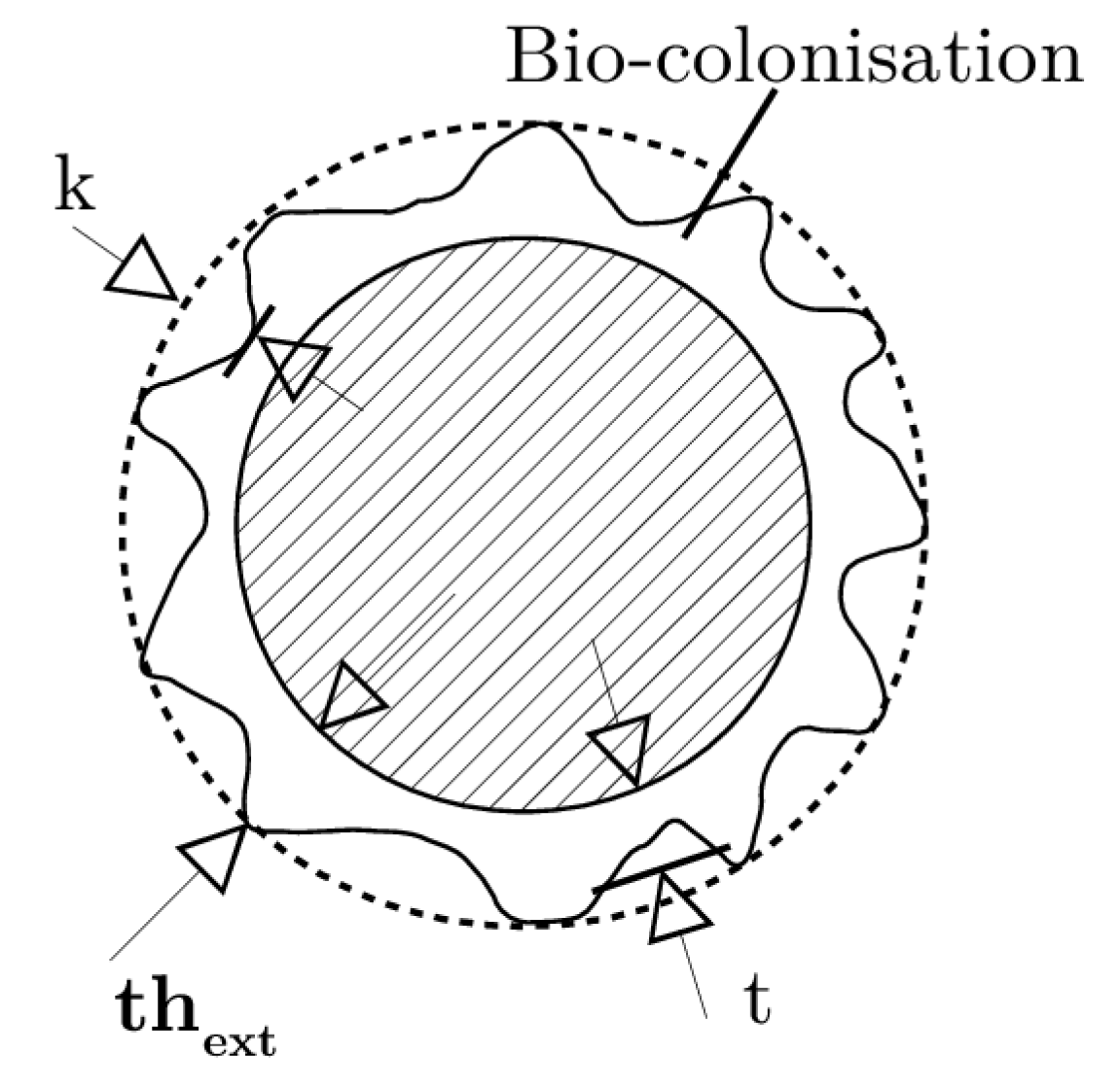
Previously introduced data, which were used to build the thickness spatial model, enable to set up a local model for SEMREV test site that could be generalised by introducing stochastic parameters of the model.

2.1.2. Modelling

The purpose of modelling is to highlight configurable phenomena of thickness distribution along the mooring line.
Three phenomena are then clearly observed:
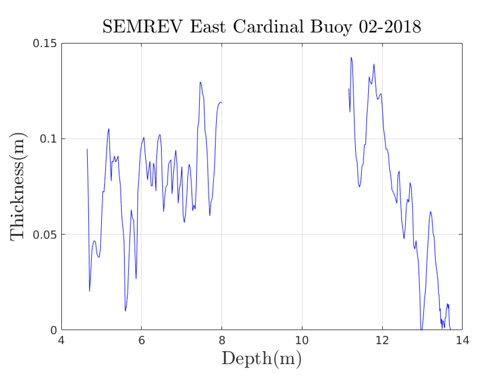
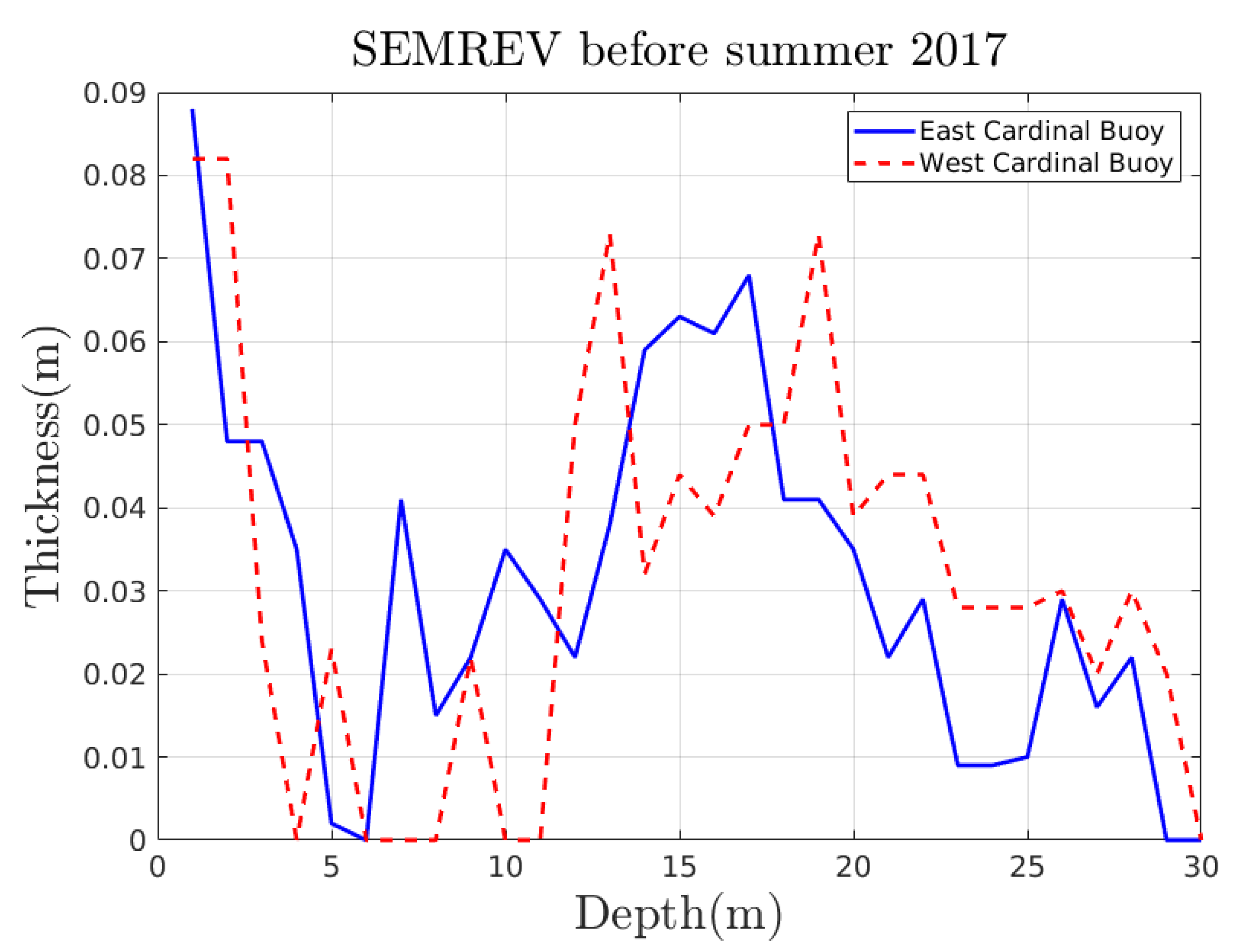
  • A decrease of thickness with depth.
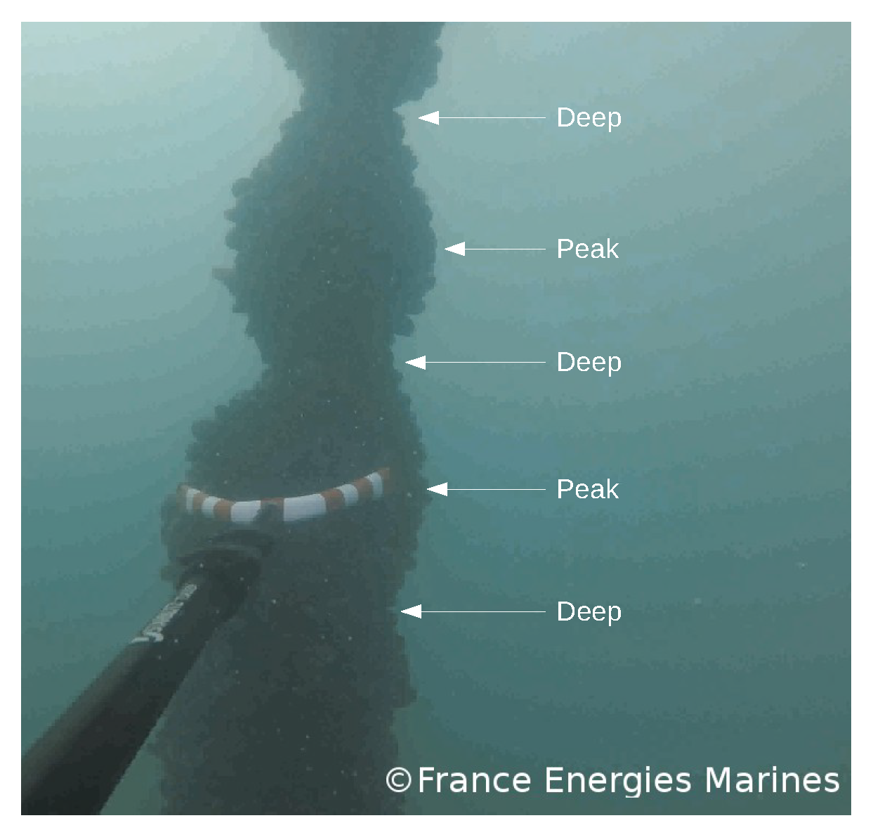
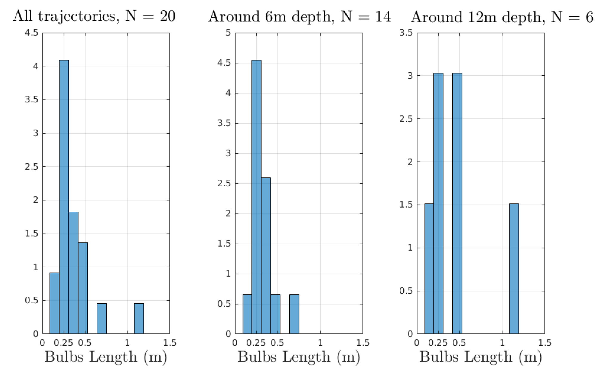
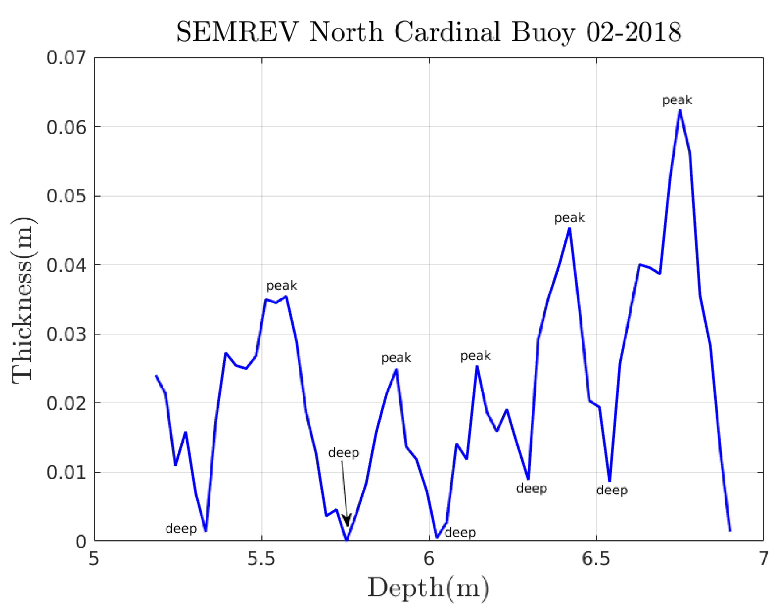
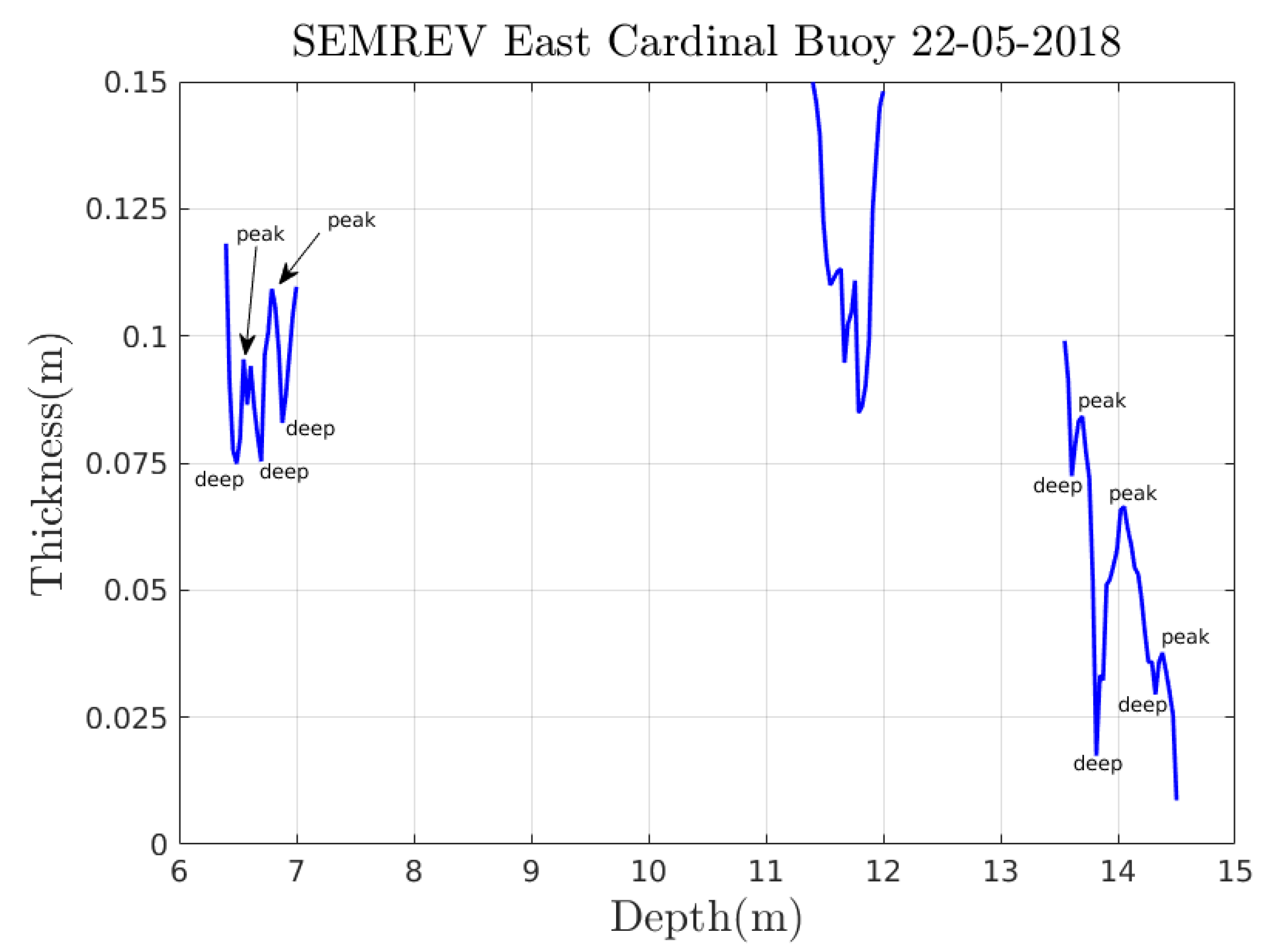
  • The emergence of bulbs or lumps identifiable by peaks and deeps of thickness along the line.
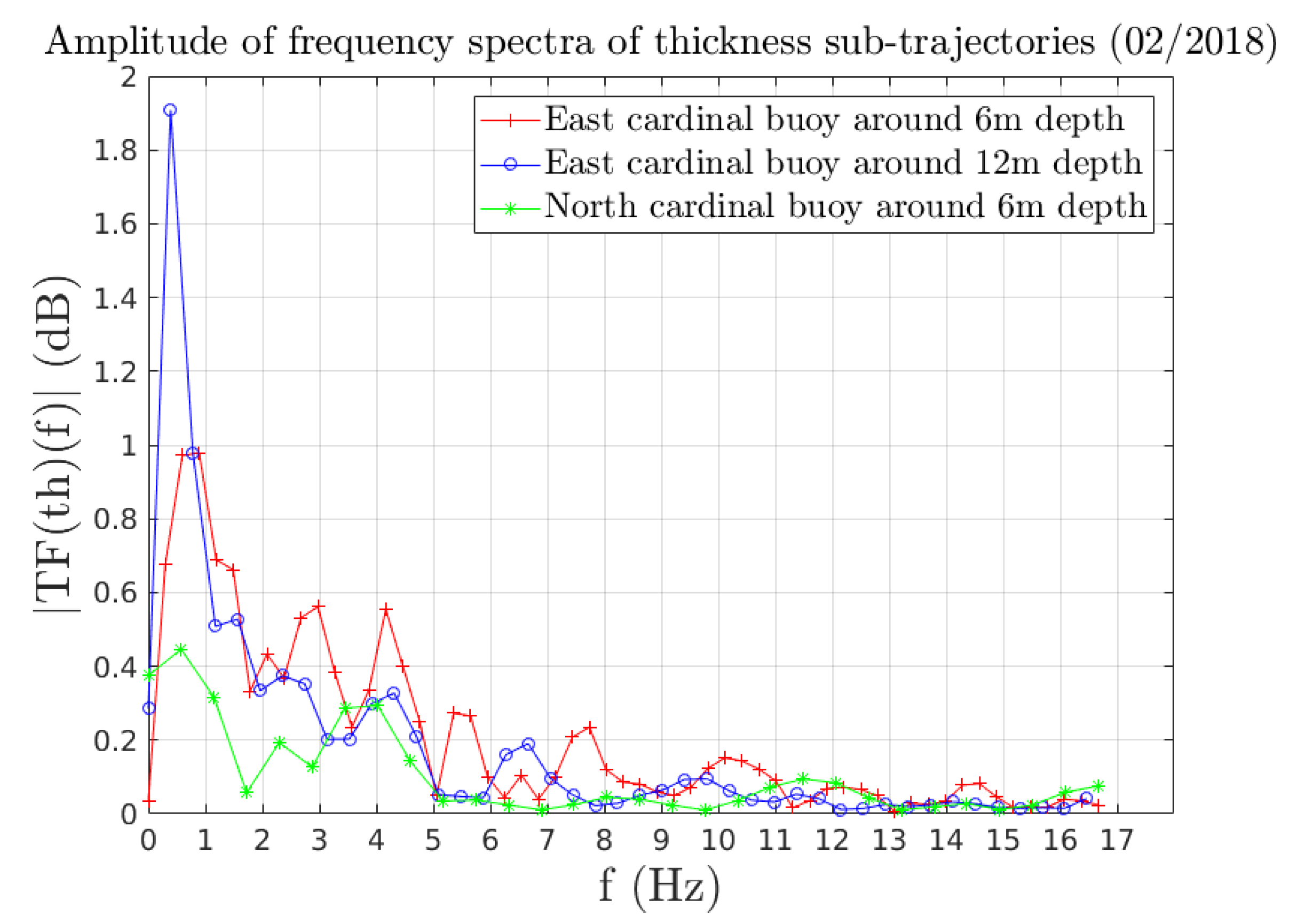
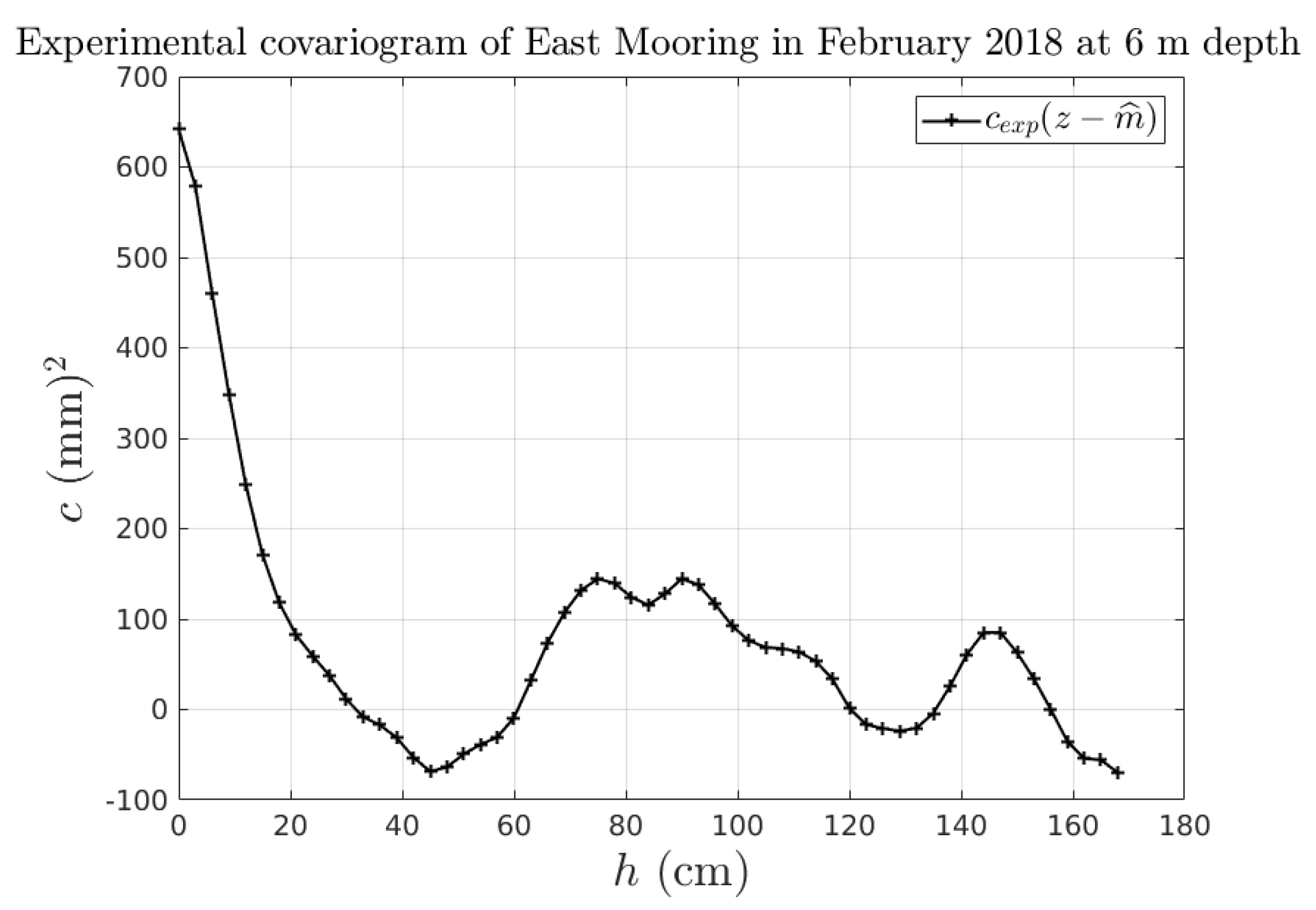
  • A correlated geospatial process.
The joint evolution of biotic (interaction between species) and abiotic (temperature, food availability, etc.) parameters with depth explains the decrease of thickness with depth. Light intensity is decreasing with depth. A lower input of light makes the photosynthesis more difficult. Therefore, biological concentrations of phytoplankton, of microphytobenthos and macro-algae are decreasing. However, the latter are the main food of filtering molluscs such as mussels. So the concentration of mussels decreases with depth and so is the thickness [4].
We noticed the emergence of bulbs of mussels on videotapes from diving missions. Figure 6 shows bulbs, which are marked out by deeps. Between two deeps, the bulb has a peak of thickness.
The frequency analysis carried out on dense sub-trajectories - to avoid the influence of a gap of several meters, from processed videotapes by pointing, attests to this emergence phenomenon. Please note that both trajectories from Spraul et al. [8] have a discretisation step of 1 m, which is too wide to catch the spatial frequency of bulbs. Three sub-trajectories, whose length is greater than 1.5 m, were re-sampled with a constant spatial period of 3 cm and the Discrete Fourier Transform (DFT) of the residuals of the sub-trajectories was calculated using an FFT algorithm. Their frequency spectra are plotted in Figure 7.
We focus on the residuals, instead of the thickness itself, to erase the peak of frequency at f = 0 and to prevent from its secondary frequencies. Thickness is a real value, so the magnitude of its DFT is even. Therefore, only the positive part of the frequency axis was plotted. Moreover, the DFT is a periodic function, of period 1 T C with T C = 0.03 m. Then, only the half-period [ 0 ; 1 2 T C ] was plotted. Spectra are converging to 0 when f 1 2 T C , which proves that the sampling period T C is low enough and that the Shannon condition is fulfilled.
Figure 7 shows a principal peak of frequency around 0.5 Hz, which is equivalent to a wavelength of 2 m. The non-stationarity of sub-trajectories can explain this peak. Then, one can notice the emergence of other frequencies between 3 and 4 Hz, which is equivalent to wavelengths around 0.3 m. It will be shown later that the length of most bulbs is around 0.3 m. Then the frequency analysis confirms the emergence of bulbs of mussels whose length is below 1 m.
The last phenomenon introduced in the model is that residuals of thickness spatial distribution can be thought of as a Gaussian and stationary correlated geospatial process around a non-stationary mean, the decreasing trend as previously introduced. The work of Ameryoun et al. on the modelling of mussels growth with a temporal Gamma process ([4] in Chapter 2, [14]), shows a temporal convergence of the distribution of shells length to a Gaussian distribution. The thickness is made up of the sum of individuals length. It is, therefore, reasonable to consider the thickness as a Gaussian spatial process.
This assumption was checked thanks to the work of Clerc et al. [21] and it also enabled choosing a type of auto-covariance function. The SCAP-1D algorithm developed by Clerc et al. [21] checks if the hypotheses of stationarity (second order stationarity) and normality of the proposed trajectory are true or not. It also measures, through the Akaike Information Criterion (AIC) [22], the relevance of the chosen model of the auto-covariance function, which is an input to the SCAP-1D algorithm. The model should represent the experimental auto-covariance function. Four of the five available trajectories were analysed. “North Mooring in February 2018” (cf. Figure A3) is too short to be relevant for SCAP-1D analysis. The χ 2 test and the Kolmogorov-Smirnov (KS) test are checking the normality. It was shown that the hypotheses of stationarity and normality are true for the four trajectories. Please note that when it was possible, hypotheses were tested directly on experimental trajectories, otherwise they were tested on the model estimated from the trajectories thanks to a Maximum Likelihood Estimation (MLE) or a Least Squares Estimation (LSE). The auto-covariance function minimising the AIC for the three trajectories is the exponential one.
The whole model of thickness distribution along a line is summarised in Figure 8.
Let us first focus on the distribution of deep-peak pairs. Figure 9, presenting thicknesses of the deep-peak pairs (with downstream peaks) picked up on experimental trajectories in agreement with the identification of bulbs on videotapes, shows that the thickness of a deep is steeply and mostly linearly correlated with the thickness of its paired peak. The Spearman’s correlation coefficient is equal to 0.78 with a p-value of 1.1 × 10 5 . Please note that the combination of deeps and peaks is centred around the decreasing non-stationary mean. In fact, we generate a non-centred Gaussian process for the peaks by using the work of Dietrich et al. [23] on the circulant embedding of the covariance matrix. As a consequence, we generate thicknesses for the deeps that are correlated one by one to the closest downstream peak’s thickness. We impose that the thickness for the deep is lower than the thickness of the peak. We cannot use tools for the generation of cross-correlated fields because of this condition of inferiority. Further explanations about the generation of the thicknesses for the deeps are given in Appendix B.

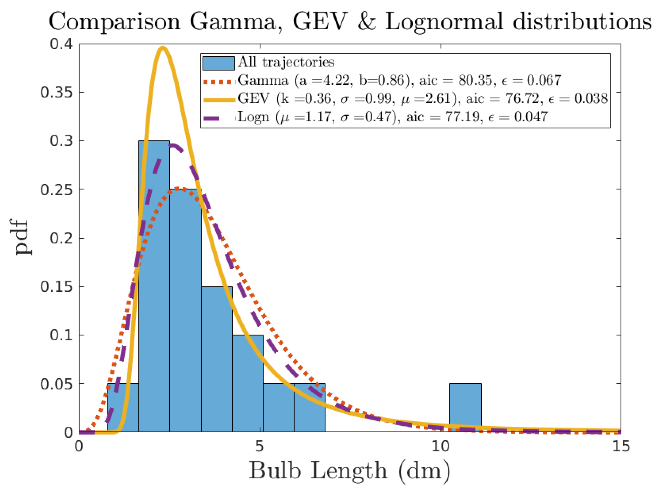
2.1.3. Parameters Identification & Model Uncertainty

The objective of this section is to specify and configure by parameters each of the boxes in Figure 8. To introduce uncertainty, some parameters are defined as random variables, following a probabilistic distribution configured by hyper-parameters. This randomising process is essential to cover uncertainties on bio-colonisation thickness at a given time. Therefore, the diversity of bio-colonisation scenarii can be represented all along the lifetime of the mooring line.
Generation of bulbs
Concerning the generation of bulbs, we extracted histograms of the length of bulbs from the five sub-trajectories from videotape processing. The length of a bulb is defined as the length between two successive deeps (cf. Figure 8). Figure 10 presents the normalised histograms got by using all sub-trajectories (N = 20 bulbs) or by grouping sub-trajectories by water depth (i.e., around 6 m and around 12 m).
The histograms of the length of bulbs have a mode around 0.25 m, which is in agreement with the results of the frequency analysis presented in the Section 2.1.2. Comparing the histograms at 6 and 12 m depths, we can conclude that the mode around 0.25 m is globally and locally inherent. It may mean that the distribution of bulb lengths is, to some extent, water depth independent. To generate bulb lengths, a model for the distribution of bulb lengths has to be selected and then estimated, to be sampled in a second phase. A Gamma distribution, a Log-normal distribution and a Generalised Extreme Value (GEV) distribution were considered to be good candidates. Thanks to an MLE, parameters of these three distributions were estimated, and two metrics were calculated to help to select the best distribution: the AIC and the mean error ϵ between the empirical cumulative density function and the estimated cumulative density function. Figure 11 presents the histogram combining all sub-trajectories along with the three estimated distributions.
The GEV distribution was retained because it is the one which minimises the AIC and ϵ . The generation of bulb lengths (cf. Figure 8) is then based on a random sampling of a GEV distribution, whose parameters are a shape parameter k of 0.36 , a scale parameter σ of 0.099 m and a location parameter μ of 0.261 m. To prevent the generation of too short bulbs, the GEV distribution is truncated by a lower limit of 0.1 m. Indeed, the minimum length observed in the trajectories was 0.18 m over 20 bulb lengths. Moreover, because of the previous remark on the scale-invariant behaviour of the distribution of bulb lengths, the distribution is not sampled by using a Monte-Carlo Sampling (MCS) but rather by using a Random Latin Hypercube Sampling (RLHS) which ensures that the distribution is locally represented. The number of equi-probabilistic intervals was chosen as L M e a n G E V with L = 5 m. It means that the distribution is represented each 5 m-length of the mooring line. L is in agreement with the length of dense sub-trajectories.
Non-stationary decreasing spatial mean
Now concerning the non-stationary decreasing spatial mean, for the lack of stronger evidence, we took the simplest model, a linear one (cf. Equation (1)). In previous works about spatial distribution of bio-colonisation on offshore structures [4,11,12,17,20,24], there is neither clear evidence of a general slope break, which would have justified a bilinear model, nor clear evidence of a slowing down of the rate of decrease, which would have justified an exponential model.
t h m e a n ( s ) = a + b . z ( s ) ; a > 0 ; b < 0 ; z > 0 ; s > 0 .
with, z the vertical depth (cf. Figure 8), defined positively from the MWL to the seabed. s represents the curvilinear abscissa along the mooring line from the fairlead to the anchor. We used four trajectories out of the five available ones (NB: “North Mooring in February 2018” (cf. Figure A3) is too short to be relevant for estimating the decrease) to identify the two parameters, a and b of the linear model (Equation (1)) by using a weighted LSE. We chose weights ( W ) to gradually favour parts where the growth of bio-colonisation is more permanent in time, so more representative of the mean thickness. Thus, thickness from 0 to 6 m depth were favoured ( W 1 = 10 4 ) compared to thickness from 6 to 15 m depth ( W 2 = 4.44 × 10 3 ), which were also favoured compared to thickness from 15 m depth to seabed ( W 3 = 2.5 × 10 3 ). Table 1 presents the estimated values for a and b, along with their 95 % confidence bounds, calculated by the fitting algorithm (Levenberg-Marquardt):
Based on these results, we chose probabilistic distributions for a and b, because they differ significantly from a case to another; they are also leading parameters for the mass distribution of bio-colonisation along the mooring line. To understand our choice for the distributions of the now random variables a and b, their physical meaning has to be kept in mind. Looking at Equation (1), a represents the mean thickness at the first point in water of the mooring line. b represents the rate of decrease of the mean thickness with depth and is expressed negatively. Distributions of a and b lead the diversity of the mass distribution scenarii in time. There is no evidence to favour in time a scenario rather than another. Moreover, even if the model is initially calibrated on site-specific data, our intent is also to cover the diversity of sites colonised by mussels. Therefore, we adopted uniform distributions, which are the less informative distributions. The lower limit of a is equal to 1 cm, which represents the beginning of a discernible juvenile colonisation. The upper limit of a is equal to 20 cm, which is an upper approximation of the upper confidence bound of the colonisation on the “East Mooring” in May 2018 (cf. Table 1). This upper bound agrees with observations in [17] and [19] (p. 19), noting that mussels colonisation in Atlantic area can reach a thickness of 15–20 cm. The lower limit of b should represent a quick decrease. Based on feedback from mussel farmers, it may be that in some regions close to the coast, due to a high turbidity, the mussels colonisation stops after 5 m depth. With a mean thickness at MLW of 10 cm, it represents a b-value of 0.02 . On the other hand, the upper limit of b should represent a slow decrease. Mussels have once been found at a depth of 99 m during inspections on a jacket in the North Atlantic Sea [24]. Thus, it is possible, it is highly unusual. A slow decrease is then a colonisation which stops around 60 m. With a mean thickness at MLW of 10 cm, it represents a b-value of 0.017 , which is close to the mean value of the colonisation on the “East Mooring” in February 2018 or the lower confidence bound of the colonisation on the “East and West Mooring” before summer 2017 (cf. Table 1). Distributions of a and b are summarised at the beginning of Section 2.2.2, where all the parameters are gathered.
Generation of a Gaussian field for the residuals
Now regarding the generation of a random field for the residuals, we showed in the modelling that a Gaussian and stationary process with an exponential auto-covariance function is a suitable representation for the residuals:
t h r e s i d u a l s N μ r e s i d u a l s = 0 ; σ r e s i d u a l s ; c ( h , l c ) ; c ( h , l c ) = σ 2 e x p h l c .
First note that we base our following analysis on the fact that some observations of the geospatial process can inform about parameters of the process. This is true if trajectories are ergodic. Please note that the ergodicity of experimental trajectories was problematic to assess due to either a low density of measurements points or the wide gap between measurement zones. However, the ergodicity of sub-trajectories of dense trajectories, such as “East Mooring in February 2018” at 6 m depth, has been assessed by checking if their experimental covariogram tends to zero [21].
The experimental covariogram of the sub-trajectory in Figure 12 oscillates around zero. The sub-trajectory is then ergodic and by estimating the parameters of this sub-trajectory, we estimate the parameters of the geospatial process. Thus, we think the estimated values in Table 2 are representative of the geospatial process for residuals. Please note that these parameters are estimated on “full” experimental trajectories, not only on trajectories of peaks which are not dense enough. Nevertheless, they are used to generate the non-centred Gaussian thickness process for the peaks. Peaks are a subset of “full” trajectories and so we hypothesise they follow the same multi-dimensional law.
In Equation (2), μ r e s i d u a l s is the constant mean of the marginal Gaussian law of the process. It is equal to 0 because residuals are centred around the decreasing linear trend (cf. Equation (1)). σ r e s i d u a l s is the constant standard deviation of the marginal Gaussian law of the process. c ( h , l c ) is the exponential auto-covariance matrix of the process. Please note that μ r e s i d u a l s and σ r e s i d u a l s are constant because the process is stationary (at least second order stationary). The auto-covariance function is the function equal to the covariance of the pair of random variables ( t h r e s i d u a l s ( s ) , t h r e s i d u a l s ( s + h ) ) . Yet the process is at least second order stationary, so the auto-covariance function depends on the difference ( s + h ) s = h . The correlation length parameter, l c (m) in Equation (2), is a parameter of the auto-covariance function. An interpretation of l c is the spacing h for which thicknesses from two points along the line spaced by h are faintly correlated. So that the correlation between those two points is considered negligible. Thanks to the SCAP-1D algorithm [21], four of the five available trajectories were analysed. σ r e s i d u a l s (or σ r e s i d u a l s 2 with SCAP-1D) and l c have then been identified for each trajectory along with their 95 % confidence bounds. The following table presents the results along with the method of identification, MLE or LSE [21].
Please note that the discretisation step is equal to 1 m for the first two trajectories in Table 2. Therefore, the correlation length, l c , estimated for these two trajectories is biased because it cannot be lower than the discretisation step. Based on Table 2, we chose to randomise σ r e s i d u a l s and l c , because of their wide 95 % confidence intervals (except for the LSE). Contrary to a and b, which vary significantly in time and from a site to another in correlation with environmental parameters, σ r e s i d u a l s and l c are closely linked to the species of colonisation and their self-organised spatial patterning. Therefore, we adopted normal distributions, which are more informative than uniform distributions, but still symmetric. Normal distributions are truncated by a lower limit and an upper limit to prevent future sampling of unrealistic values. The mean of the normal distributions is centred between the limits and the standard deviation of the normal distribution is chosen as the quarter of the difference between the upper and the lower limits. The truncated normal distributions are therefore defined on the 95 % confidence interval of the normal distributions. The lower limit of σ r e s i d u a l s is extracted from Table 2 (line 2, East Mooring before summer 2017, lower confidence bound) as σ r e s i d u a l s 2 and is equal to 0.008 m. The upper limit of σ r e s i d u a l s is equal to 0.06 m (East Mooring in May 2018, upper confidence bound). The upper limit of l c is equal to 2 m, which is an approximation of the upper confidence bound of l c on line 4 of Table 2. Table 2 cannot help to choose the lower limit of l c because lower confidence bounds are negative or not informative in the LSE case. Based on the physical interpretation of l c , we have judged that inside a bulb, thicknesses are significantly correlated. Therefore, l c should at least be equal to 0.2 m, which is a lower approximation of the mode of the GEV distribution of bulb lengths. The distribution of l c includes the hydrodynamic correlation highlighted by Molin [25] (p. 158), and estimated to be equal to several diameters of the mooring line. It is important since the correlation length of the bio-colonisation could impact the hydrodynamic correlation, which impacts the Vortex Induced Vibrations (VIV) of the mooring line. Distributions of σ r e s i d u a l s and l c are summarised at the beginning of Section 2.2.2.
The parameters of the spatial model of bio-colonisation thickness are not correlated with each other. There is not for now enough data to evaluate any correlations. Moreover, there is no biological motivation to correlate parameters. For instance, the colonisation may be profuse in the first meters under MWL and may decrease either very quickly or very slowly. So a and b seems intuitively hardly correlated.
To use this model in a monitoring frame, based on tension monitoring in calm sea states and so based on the mass distribution of bio-colonisation, our hypotheses about the values of bio-colonisation density have now to be clarified. Density is necessary to go from thickness distribution to mass distribution of bio-colonisation.

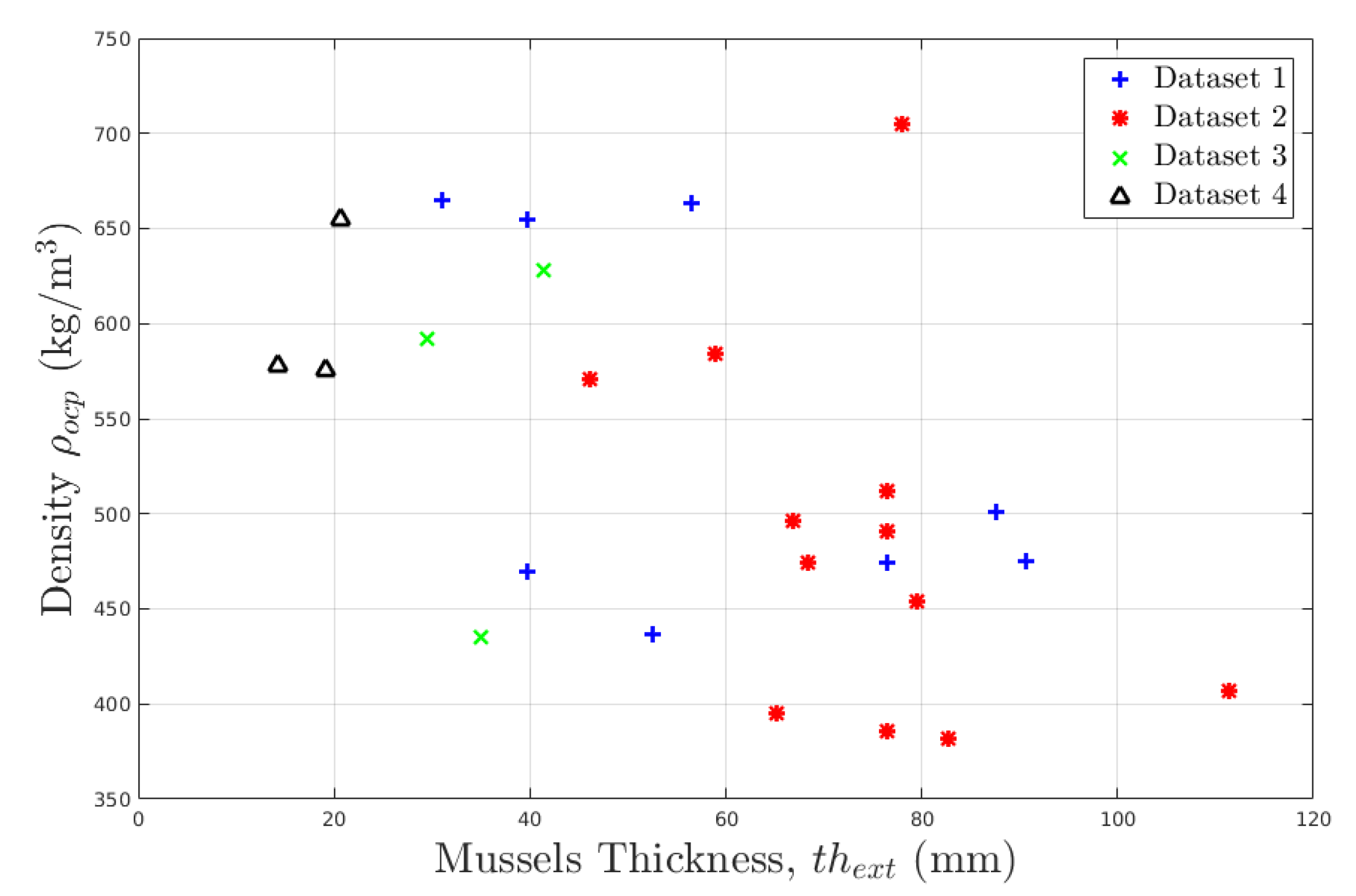
2.1.4. Density of Bio-Colonisation

It is first important to note that in this work, density( ρ ) is expressed in kg·m 3 , unlike in biology where people used to express it in kg·m 2 (areal density, A d ). Because we are modelling first a thickness and then a mass, so first a volume and then a mass, density has to be expressed in kg·m 3 . Please note that we chose to compute mass distribution from thickness distribution, and not the contrary, because our database is a visual database which enables us to extract only the thickness.
Before introducing an a priori distribution of the density, we have to define the different densities, ρ that can be measured when considering a sample of mussels and to select one. Let’s first describe a cluster of mussels and a mussel.
As sketched in Figure 13, when mussels cluster around a rope, due to their concave shell, they do not fill all the space but rather create interstices full of water. This water is then called the interstitial water. Mussels are filtering animals. Therefore, when submerged in a sea current, they are open most of the time to filter the freshwater brought by the current. When necessary, usually when they feel in danger, they can close themselves, using internal muscles. When closed, they keep some water inside their shell. This water is called the intervalvular water.
By taking mass and/or volume of these waters into account () or not (×), several densities can be defined. Note first that the volume of the intervalvular water is a volume trapped in mussels shell that we do not consider. Note then that the mass of interstitial water is not of interest because the weight of this water is equal to its buoyancy and so it does not weigh on the line. Table 3 presents the three densities.
The three densities follow the relationship: ρ o p < ρ o c p < ρ c p . The one in which we are interested in for engineering purpose is ρ o p because most of the time, mussels are open. However, the quantification of the mass of a cluster without intervalvular water mass is not an easy task and quite approximate. In the following, ρ will be then based on ρ o c p . It can be considered to be a conservative approach since intervalvular water represents around 20 % on average of the total mass (without the mass of interstitial water).
For the sake of simplicity, density is considered homogeneous along the mooring line and independent from the thickness. Moreover, we cannot arbitrarily correlate it with any thickness model parameters. Based on four datasets of the measurement of ρ o c p (cf. Figure 14), we have decided to model the density of bio-colonisation as a random variable, ρ , which follows an a priori uniform distribution between 300 and 800 kg·m 3 for embracing the variability with time of probable layouts between juvenile and adult mussels. It is actually difficult to forecast the evolution of these layouts with time. Nothing can biologically justify a more informative a priori distribution. The first two datasets are extracted from the work of Anne-Laure Barillé in 1993 and 1994. The last two datasets are based on experimental campaigns carried out in 2019.
This last section about the a priori density of bio-colonisation puts an end to our a priori spatial model of bio-colonisation. We derived an a priori spatial model for the thickness, which is configured by four variable parameters (a, b, σ r e s i d u a l s and l c ), each of them following a probabilistic distribution. This model is based on in situ data from the SEMREV test site and is specific to mussels colonisation. In addition, we carried out an experimental campaign with a mussel farmer to calibrate an a priori model for the bio-colonisation density ( ρ ). Because bio-colonisation may have a quick temporal evolution, we are now going to estimate the ability of a tension sensors network on mooring lines to help to reduce the uncertainty (entropy) of our a priori model in a case when the sea is calm.

2.2. Reduction of the Uncertainty of our Prior Model

Our a priori spatial model is covering the seasonal and inter-annual variations of bio-colonisation thanks to a large uncertainty on its parameters. Whether bio-colonisation is showed as a non-negligible phenomenon for the fatigue of the mooring lines of a specific Floating Wind Turbine (FWT) design, it is then necessary to decrease the uncertainty on bio-colonisation parameters during the life of the FWT before re-assessing the remaining lifetime of the mooring lines. In fact, the non-monotony of the temporal evolution of bio-colonisation (cf. [12]) makes its prediction difficult. Phenomena that could be responsible for the non-monotony, are:
  • the storms which can result in high accelerations and vibrations of the mooring lines and so lead to the unhooking of mussels clusters.
  • the natural unhooking of multi-layered mussels clusters when they reach a critical size. The external layers can come down during a slack event of the line due to their fragile connection with below layers, which are directly hooked to the mooring line. This phenomenon is well-known by mussel farmers, who remove these external layers before they come down and let the underneath mussels grow.
  • the mortality due to attacks of predators such as sea stars (Asterias rubens) or sparus fishes (Sparus aurata).
  • the non-monotonous supply of phytoplankton which is depending on phytoplankton bloom and currents.
  • The mortality or growth due to extreme variations of environmental parameters such as temperature.
  • Pollution or diseases.
We thus propose in this paper a simple strategy to update the parameters of our a priori model, at least once a year based on sea states. When the sea is calm (barely any wave height, and very low wind and current velocities), the dynamics of the floater around its equilibrium position is very low, the floater is static and so the tension in a mooring line only depends on the applied pretension and mooring line weight in water. The pretension is applied during the installation phase and known up to a certain level (uncertainties due to installation for instance). The mooring line weight is composed of the own weight of the line (without bio-colonisation), known up to a certain level of uncertainty and pointed out by the manufacturer, and of bio-colonisation weight in water. The only unknowns are then the tension in mooring lines during a calm sea state and bio-colonisation weight in water. These unknowns are linearly linked because, in a calm sea state, the action of bio-colonisation mass on the tension is only due to its weight. Therefore, by measuring the tension during a calm sea state, the weight of bio-colonisation on the line could inversely be deduced. The linear relation linking tension and biomass is monotonous and solving an inverse problem would lead to a unique solution. Moreover, if several tension sensors are distributed along the line, the distribution between sensors of the total mass can be deduced. This is a first essential step in our updating strategy.
A calm sea state is now considered to be a Qualifying Sea State (QSS) for bio-colonisation. This QSS is theoretically defined as a sea state for which the influence of bio-colonisation mass in the tension of the mooring line is greater than the one of each environmental parameter. It is presumed that such a sea state is a calm sea state, meaning low intensity of environmental parameters. This point will be further investigated in future works.
Our purpose is to reduce uncertainty on the parameters of our a priori spatial model, which is not based on mass distribution but on thickness distribution. We then propose, in this paper, to build the posterior distributions of the parameters of our model by Monte-Carlo Sampling (MCS). By sampling values of our parameters for the thickness spatial distribution and for the density, following their probabilistic prior distributions, we can generate bio-colonisation mass distributions along the line and thus select those which fit in with the deduced mass distribution from tension measurements. Each selected mass distribution matches with a sampling array of parameters ( a i , b i , σ r e s i d u a l s , i , l c , i and ρ i ). By an MCS approach, we then obtain a sampling of posterior distributions of parameters for the thickness spatial distribution and for the density. Please note that if a parameter is sensitive to the updating, its posterior distribution has a lower uncertainty than its prior one. By estimating the decrease in uncertainty, we can assess the efficiency of the updating strategy and so of the configuration of sensors. To study this efficiency, we will:
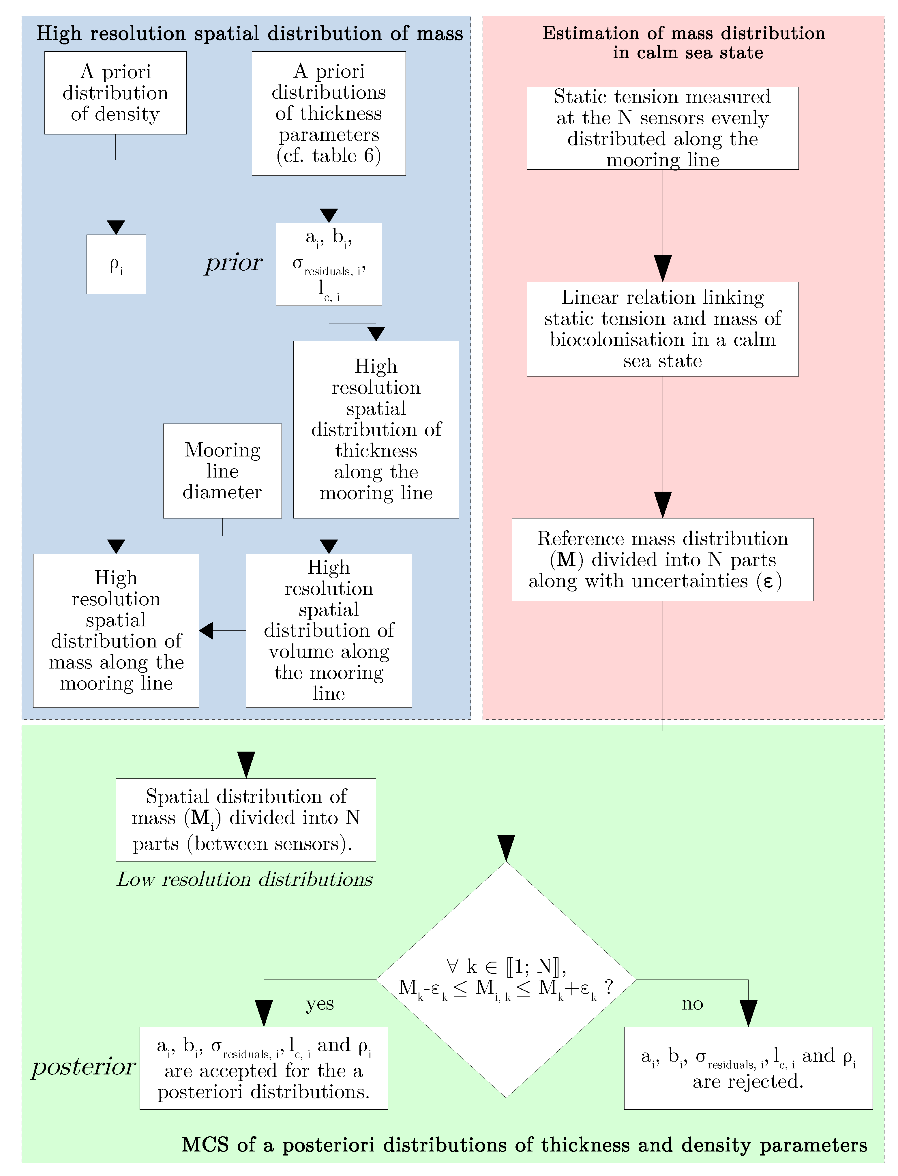
  • define a realistic case study by presenting the chosen anchoring geometry, by configuring a tension sensing network on it and finally by proposing different realistic scenarii of bio-colonisation called reference mass distributions.
  • present the methodology to build samples of posterior distributions of thickness and density parameters, which will depend on the number and the measurement error of tension sensors, and also on the reference mass distribution of bio-colonisation.
  • introduce a robust estimator to quantify the reduction of uncertainty between prior and posterior distributions.

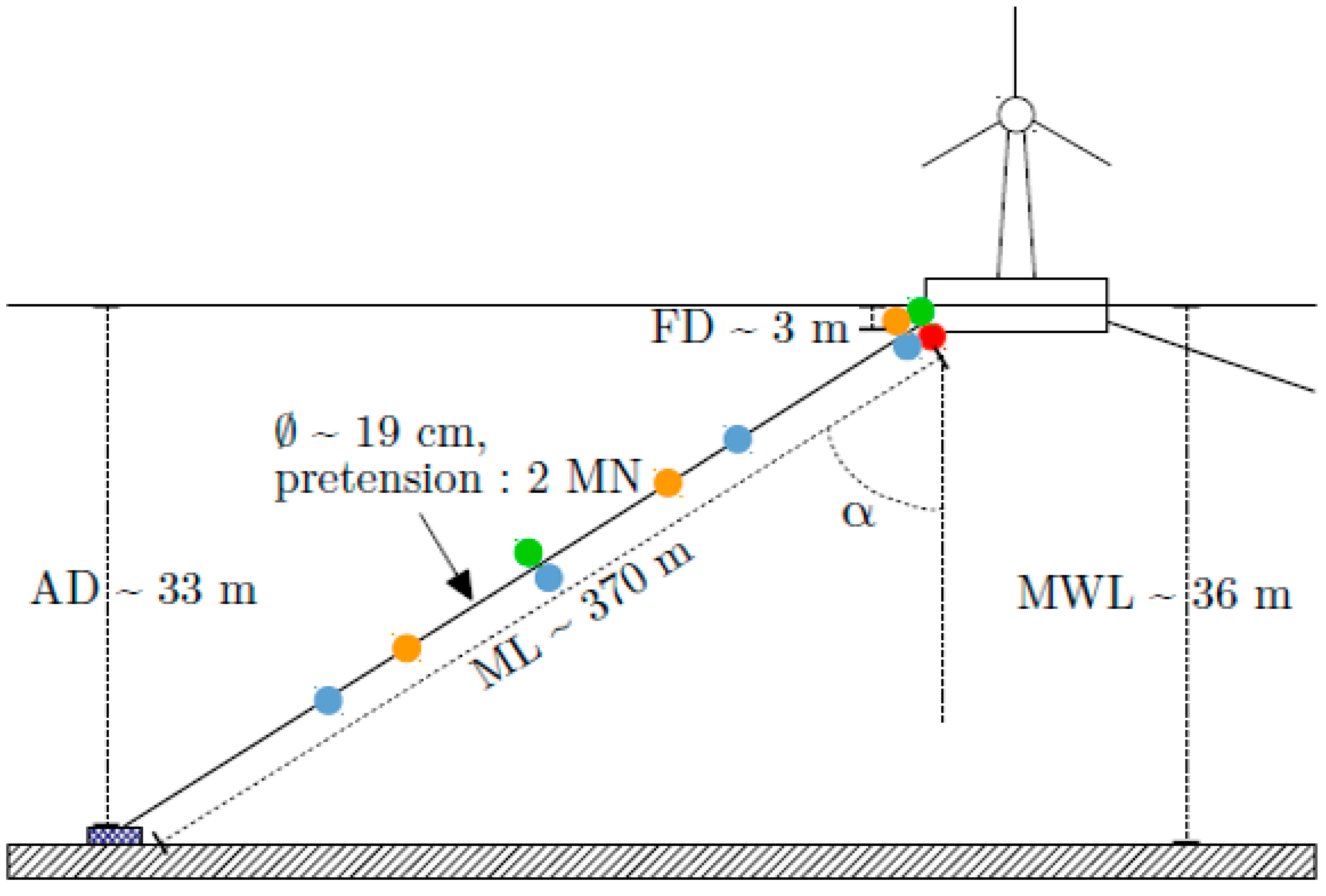
2.2.1. Realistic Mass Distributions of Bio-Colonisation and Parametrisation of Distributed Sensors on a Monitored Mooring Line of a FWT

It is first to be noted that a FWT has been preferred to a Floating Production Unit (FPU) for the application of the methodology. FWTs intend to be installed in shallower water and closer to the shore than FPUs are, with relatively smaller mooring lines diameter. For all these reasons, it is believed that bio-colonisation mass will be higher on FWT proportionally to the mooring length and volume. In this paper, the proposed methodology is thus intended for FWTs.
We consider a FWT located offshore of Nantes (on the SEMREV test site or further on the west coast of France), where colonisation is shown to be dominated by mussels. We chose an anchoring geometry of a barge in about 36 m water depth [8] for our case study. This barge has seven mooring lines: three front and four rear mooring lines. The case study is focused on one the rear mooring line, whose length is 370 m (Mooring Length, M L , cf. Figure 15). The MWL of the installation site is 36 m depth. Fairleads are approximately 3 m underneath the MWL (Fairlead Depth, F D ). Mooring lines are linked with anchors approximately 3 m above the seabed, being 33 m depth (Anchor Depth, A D ). Mooring lines are divided into three sections: chain-nylon-chain, respectively from fairlead to anchor to avoid friction and abrasion of nylon with the floater and the seabed. For simplicity, in this paper, mooring lines are only composed of a 19 cm ⊘ nylon rope, which are taut with a 2 MN pretension and whose mass per unit length is equal to 31 kg·m 1 . The curvilinear abscissa along the line, s, is defined from the fairlead to the anchor and the deformed shape of the taut mooring line z ( s ) (cf. Equation (1)) is given by the anchoring geometry:
z ( s ) = s A D F D M L + F D .
with z defined downward positively from MWL. Please note that Equation (3) is only valid for the present case of a taut and linear mooring line. Four different configurations of the tension sensing network are considered in this paper:
  • Only one tension sensor close to the fairlead (red in Figure 15).
  • Two tension sensors (green). One close to the fairlead and a second in the middle of the line.
  • Three tension sensors (orange). One close to the fairlead, a second at one-third of the line and a last at two-third of the line.
  • Four tension sensors (blue). One close to the fairlead, a second at one-quarter of the line, a third in the middle of the line and a last at three-quarter of the line.
These four designs of sensor distribution are representative of realistic strategies, from the simplest and cheapest (one sensor) to a significantly dense one (four sensors). Please note that for each configuration, sensors are evenly distributed along the line. Please note that the technological aspects of sensors are not discussed in this paper. We consider that the measurement of tension and the relaying of information at the aforementioned positions are possible. We also consider that sensors do not disrupt the spatial distribution of bio-colonisation. The anchoring geometry and the four configurations are sketched in the following figure.
The objective is now to build virtual realities of four scenarii of mass distribution. They were generated by choosing given potential values of thickness and density parameters. By choosing thickness parameters ( a r e f b r e f , σ r e s i d u a l s , r e f and l c , r e f ), we can generate a spatial distribution of thickness along the mooring line of the case study. Considering the nominal diameter of the mooring line, considering the axis-symmetry hypothesis and linear extrapolation of thickness between deeps and peaks (cf. Figure 8), we were able to calculate the spatial distribution of volume. The volume V of bio-colonisation between a deep of thickness t h 1 and a peak of thickness t h 2 , distant from each other of l m, along a mooring line of D diameter is:
V = π l 3 t h 1 2 + t h 2 2 + 3 2 ( t h 1 + t h 2 ) + t h 1 t h 2
Since we also chose a density ρ r e f for the reference distributions, the mass distribution was easily calculated from the volume distribution. The following tables present the respective parameters (cf. Table 4) and mass distribution of distinctive bio-colonisation cases (cf. Table 5), therefore constituting reference scenarii of bio-colonisation: on an unfavorable site, on a favourable site after some months, fully developed in a favourable site and after a storm. These virtual realities define the observations extrapolated from tension measurements. We add signs to identify quickly if parameters take low , high or medium values in their respective prior distribution (cf. Section 2.2.2).
The “Unfavourable site” scenario represents a mature colonisation of adult and juvenile mussels which rapidly stops in the first quarter of the line due to unfavourable conditions. Please note that combination of adult and juvenile mussels can lead to a multi-layered and compact colonisation, and therefore to a high density (cf. Table 4). The “Favourable site after some months” scenario represents colonisation of juvenile mussels in the first months in a favourable site. Due to the low mass of each juvenile mussel in the first months and their one-layered colonisation, density is low for such a scenario (cf. Table 4). The “Full developed in favourable site” scenario represents a substantial mature colonisation after some years in a favourable site. And, the “After a storm” scenario represents a favourable site after one or two years which would have suffered from a storm, leading to the unhooking of mussels close to the MWL and so balancing mass distribution between the first and second quarter of the line.
Mass distributions are presented in Table 5 for each configuration of the tension sensing network. They are reference distributions, meaning that they represent mass distributions that should be obtained from the processing of data in calm sea state from the tension sensing network without errors of any kind. However, in reality, there are sources of error that should be taken into account in the updating of our a priori model.

2.2.2. Updating a Priori Model from Measurements

As introduced in Section 2.1.3 and Section 2.1.4, the model of mass distribution of bio-colonisation along a mooring line has five parameters: a, b, σ r e s i d u a l s , l c and ρ . We recall that the bio-colonisation spatial process is submitted to large variations in time and between settlement sites. To be able to cover these variations, the parameters have been randomised, based on experimental data and expert knowledge. The selected probabilistic distribution of each parameter is recalled in Table 6.
The diagram in Figure 16 recalls the methodology introduced at the beginning of this section. It illustrates the MCS approach used to build samplings of the posterior distributions of a, b, σ r e s i d u a l s , l c and ρ .
First, the term “high resolution” is used to qualify a spatial distribution which represents the complexity of our model by considering peaks and deeps and whose discretisation step fluctuates with the length of bulbs. To go from a high resolution spatial distribution of mass to a spatial distribution of mass divided into N (≤4 in this article) parts, we just sum all mass contributions of the high resolution spatial distribution from a sensor position to the successive sensor position (or to the anchor for the deepest sensor).
Second, an uncertainty array ( ϵ ) is introduced for the reference mass distribution obtained by inverse solving the linear relation from static tension measurements in calm sea state. The linear relation between static tension (T) and mass of bio-colonisation (M) is:
T = M + M L V L + V ρ w a t e r g . c o s ( α ) + P t
with M L and V L , respectively the mass and the volume of the line, V the volume of bio-colonisation, α the angle between the line and the vertical axis (cf. Figure 15) and P t the pretension. Please note that ρ w a t e r is the density of salt water and that V L + V ρ w a t e r g . c o s ( α ) is the Archimedes’ buoyancy.
Each term in Equation (5) could be subjected to uncertainty. Among the causes of uncertainty, we can cite:
  • installation uncertainties:
    the position of the anchor which influences α and the pretension.
    the position, orientations and draft of the floater which also influence α and the pretension P t .
  • manufacturing uncertainties:
    the length and the diameter of the mooring line which influence the mass and volume of the mooring line.
In this paper, it is considered that all terms on the right-hand side of Equation (5) are known for certain, except for M. Finally, when solving the inverse problem, we only consider the uncertainty coming from relative error Δ of tension measurement. It means that if the real tension is T, then the measured tension T ˜ could be between T 100 Δ 100 and T 100 + Δ 100 , with Δ expressed in %. The following relationship between the uncertainty ( ϵ ) on bio-colonisation mass and this relative error of measurement ( Δ ) is then obtained:
ϵ = Δ · M + Δ ρ b i o ρ b i o ρ w a t e r M L V L · ρ w a t e r + P t g · c o s ( α )
It is first to be noticed that the uncertainty ϵ on bio-colonisation mass not only depends on bio-colonisation mass but also on line parameters which influence the tension. Indeed, tension measurements cannot differentiate between each contribution. Due to the high value of pretension in our case study, it is likely that the following analyses may not be sensitive to mass distributions. Therefore in the following, we consider that the pretension is null, which could be for example the case for a catenary mooring. Please note that ρ b i o is equal to 1325 kg·m 3 because the Archimedes’ buoyancy of the interstitial water is null, meaning that V is the volume of bio-colonisation empty of interstitial water.
From now on, a “scenario” (S) is more broadly defined as a combination of a reference mass distribution, a configuration of the sensing network and a relative error Δ of tension measurement. For each scenario, it is now feasible to build samplings of posterior distributions of thickness and density parameters. A robust estimator to quantify the reduction of uncertainty between prior and posterior distributions for each scenario S is now introduced.

2.2.3. Estimate for Uncertainty Reduction from SHM

The conditional entropy metric, commonly used for sensor placement optimisation (cf. [26]) was chosen. This metric is defined as:
m X | S H ( X ) H ( X | S ) | H ( X ) |
where X can be any random variable (a, b, σ r e s i d u a l s , l c or ρ ), H ( X ) is the prior differential entropy of X and H ( X | S ) is the posterior differential entropy of X for scenario S. The differential entropy of a continuous random variable X following a probability density function f and whose support is a set X , is defined as:
H ( X ) X f ( x ) l n [ f ( x ) ] d x
In this paper the base of the logarithm is e, meaning that l n is the natural logarithm, and so that differential entropy is expressed in nats. Differential entropy is an information-theoretic measure of uncertainty because it is the expected value of the information content I X ( x ) l n [ f ( x ) ] .
Please note that H ( X | S ) H ( X ) , where the equality holds only if the posterior distribution is independent of S. This implies that m X | S is always positive. Note also that the greater m X | S the more uncertainty is reduced. This is useful to compare the impact of scenarii on a specific parameter or to compare the sensitivity of several parameters to a specific scenario.
Prior distributions of thickness and density parameters are well defined (cf. Table 6). Therefore, their exact differential entropy is calculated following the definition (cf. Equation (8)). Table 7 gives the differential entropy of uniform and truncated normal distributions:
On the contrary, our methodology to update thickness and density parameters (cf. Figure 16) compels us to estimate H ( X | S ) the differential entropy of posterior distributions. Following the methodology, posterior distributions obtained for each scenario are only representative samplings. We opted for a non-parametric estimation of differential entropy which avoids calibrating a parametric model for the posterior samplings. Please note that calibrating a parametric model is risky when the size of the sampling is small or when the histogram of the sampling does not fit with any common probabilistic law. Györfi et al. made a review of non-parametric differential entropy estimators in [28]. We kept estimates with mean square consistency at least. Two different estimates were considered to strengthen the estimation: the resubstitution estimate and the cross-validation estimate [29]. They are both based on the non-parametric density estimate of the histogram of the samplings. Mean square consistency and strong consistency [28] are respectively valid for the resubstitution estimate and the cross-validation estimate when using kernel density estimate. In order to have an idea about the influence of the size of the sampling on these estimates, convergence studies were carried out. Following GEV, Weibull and uniform distributions, whose exact differential entropy can be calculated [27], we generated samplings of different sizes and estimated differential entropy of each sampling with both aforementioned estimates. Please note that normal kernels were used.
The convergence studies showed that samples of size larger than 40 are required. Because the cross-validation estimate is greater than the resubstitution estimate for small samples and equivalent to the latter for large samples, we will only keep the cross-validation estimate in the following. This is indeed a more conservative approach if our purpose is to reduce differential entropy.
The following section presents results about the influence of the sensing network and measurement error on the reduction of differential entropy of prior distributions of thickness and density parameters.

3. Results and Discussion

This section lingers over three questions:
  • On which parameter uncertainty (a, b, σ r e s i d u a l s , l c or ρ ) does the proposed methodology (cf. Figure 16) act?
  • Does the uncertainty narrow around the reference value (cf. Table 4)?
  • For parameters whose uncertainty is reduced, is the metric linked with: the reference case? The error of measurement? The number of sensors?
Before answering these questions, scenarii that are excluded from analysis are given in Table 8. Due to computing power, it has sometimes been difficult to fulfill the requirement of at least 40 samples. In fact, when the number of sensors increases and the relative error Δ of tension measurement decreases, then most of the candidate mass distributions are rejected during the MCS process (cf. Figure 16).
So we retained 56 scenarii of the 64 possible scenarii (4 reference colonisations × 4 configurations of the sensing network × 4 relative errors Δ ). For each of these 56 scenarii, the conditional entropy metric defined in Equation (7) was calculated for each parameter (a, b, σ r e s i d u a l s , l c and ρ ). The efficiency of the methodology (cf. Figure 16) is then assessed for each parameter.

3.1. Efficiency of the Methodology

Figure 17 and Figure 18 present the histogram of the conditional entropy metric for each parameter (a, b, σ r e s i d u a l s , l c and ρ ), obtained by considering all 56 scenarii.
We should first recall that the metric is theoretically greater than 0 unless the posterior distribution is independent of the scenario. Indeed, in case of independence, the posterior distribution is equivalent to the prior one and so the posterior differential entropy is theoretically equal to the prior differential entropy. Yet the estimator tends to over-estimate posterior differential entropy, leading to possible negative values of the metric in case of independence. Moreover, this over-estimation increases with the decrease in the size of posterior samplings. The occurrence of a negative value is due to an error of estimation of posterior differential entropy in case of independence.
We should then recall that the higher the metric, the higher the reduction of uncertainty. Figure 17 and Figure 18 let us conjecture that the methodology is efficient to reduce a, b and ρ uncertainties. On the contrary, the methodology seems inefficient to reduce σ r e s i d u a l s and l c uncertainties. A Student’s t-test was carried out for each parameter to check these conjectures. The alternative hypothesis ( h = 1 ) that the mean of the metric is greater than 0 was tested. The null hypothesis ( h = 0 ) of this test is thus that the mean of the metric is lower or equal to 0. Table 9 gives the result of the test for each parameter:
Conjectures are then validated by the Student’s t-test. The proposed methodology enables reducing uncertainty on a, b and ρ but not on σ r e s i d u a l s and l c . Moreover, the p-values in Table 9 do not allow a doubt about the acceptance or the rejection of the null hypothesis. This result was expected. The methodology is based on the static force induced by the mass of bio-colonisation on the mooring line. So this result makes sense since parameters (a, b and ρ ) lead the variation of mass distribution at the scale of the line. On the contrary, σ r e s i d u a l s and l c lead the variation of mass distribution at the scale of the bulbs that cannot be detected by our monitoring strategy. Therefore, unless the number of sensors is sufficient to mesh the line on the scale of the bulbs, the methodology does not enable to reduce uncertainty on σ r e s i d u a l s and l c . In the following, the latter parameters will not be considered. The p-values are also useful to rank a, b and ρ respectively by decreasing order of efficiency of the methodology to reduce their respective uncertainty. In particular, please note that the methodology is very efficient for a but faintly for ρ . Then the methodology has a relative efficiency for these three parameters, but does it enable to narrow the uncertainty around reference values (cf. Table 4)?
After the processing of posterior samplings for each of the three parameters and for each scenarii, the results are presented in the following table. The square (□) indicates excluded scenarii (cf. Table 8). () means that the mean of posterior sampling is closer to the reference value than the mean of the prior distribution is. (×) means the contrary. Cases for which the reference value and the prior mean are equal are not studied.
The ability of the method to narrow the posterior sampling around the reference value depends on the case of colonisation and on the number of sensors. Please note that it does not depend on the error of measurement. Table 10 warns us against the blind use of posterior distributions of parameters. It shows that posterior distributions obtained with our monitoring strategy do not always narrow around values that would be estimated in case the spatial distribution were known, after an inspection for example. It is comforting anyway to note that for a low colonisation (US) and for a dense colonisation (FD), the methodology enables narrowing posterior distributions around reference values for a low number of sensors. To summarise, the proposed methodology (cf. Figure 16) enables reducing uncertainties on a, b and ρ . However, we must remain watchful and critical of the use of posterior distributions of these parameters. To further guide a user of the methodology, we compare the benefits of more accurate sensors versus a denser sensor network in the following sensitivity analysis.

3.2. Sensitivity Analysis

We carried out a sensitivity analysis of the metrics for each parameter (a, b and ρ ) on the three inputs of a scenario which are the case of colonisation, the number of sensors and the error of measurement. The sensitivity analysis is based on the estimation of correlation between inputs and outputs which are the metrics of scenarii for each parameter. This method, named “Input/Output Correlation”, is the basis of sensitivity analysis. Table 11, Table 12 and Table 13 show the correlation coefficients calculated by Pearson’s method and by Spearman’s method.
Please note that the lower the p-value, the more is the confidence in the correlation. This ”Input/Output Correlation” sensitivity analysis shows that:
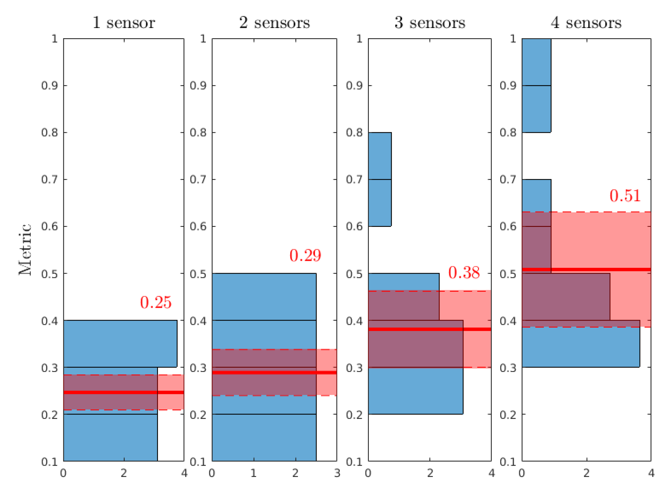
  • the reduction of uncertainty on a is strongly correlated with the number of sensors, strongly uncorrelated with the case of colonisation and uncorrelated with the error of measurement.
  • the reduction of uncertainty on b is strongly correlated with the case of colonisation, correlated with the number of sensors and dimly correlated with the error of measurement.
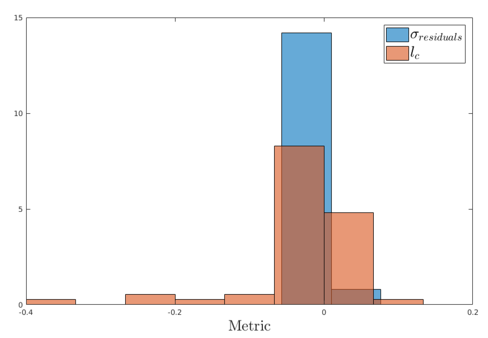
  • the reduction of uncertainty on ρ is correlated with the number of sensors, dimly correlated with the error of measurement and strongly uncorrelated with the case of colonisation.
The error of measurement does not stand out as the first influence parameter, unlike the number of sensors. Thus we advise a denser network of sensors rather than more accurate sensors in cost optimisation. However, we recommend searching for a medium accuracy of sensors to help to reduce the uncertainty on ρ . It is also comforting to note that apart from b, the reduction of uncertainty is strongly uncorrelated with the case of colonisation.
The end of our study now focuses on the influence of the number of sensors. We looked at how the metric globally changes in function of the number of sensors. This last study enables us to estimate the benefit gained on the reduction of uncertainty by increasing the number of sensors. Figure 19 and Figure 20 show histograms of the metric for parameters (a, b and ρ ), and then for a only, in function of the number of sensors.
In each case, the mean of the metric is plotted with a thick red line and its value is reported, along with its 95 % confidence interval in light red. Despite the increase of the confidence interval with the number of sensors, due to higher variability of metric sampling, we note in both cases a nonlinear increase of the mean of the metric with the number of sensors. This increase is even more noticeable in Figure 20, for which only a, the most impacted parameter, is considered. This accentuates our advice: it is better to make the network of sensors denser with a medium accuracy rather than having only one sensor at the fairlead with high accuracy.

4. Conclusions

The first part of this paper is dedicated to building a model of spatial variability for the thickness of bio-colonisation on mooring lines. It models the variation of thickness at a low scale (< 0.5 m) and in this respect, it is an original work. Unlike mostly uniform models from standards, it will then enable to study the influence of bio-colonisation variation along the line on the dynamic response of the latter. However, it is not destined to replace models from conservative standards. It could be complementary as an input for a detailed study of the effects of bio-colonisation on the fatigue of mooring lines. We also recall that the model is based on a reduced amount of data. It is thus necessary to feed it and to validate it more widely thanks to future on-site inspections. Hypotheses of homogeneous density and of axis-symmetric thickness could be reconsidered if needed.
The second part of this paper presents a methodology to update this model. This methodology is based on tension measurement at several positions along the line when the sea is calm. This static sea state is qualifying for the mass of bio-colonisation and enables reducing uncertainties on model parameters which lead the variation of mass at a line scale. However, we did not consider in our methodology uncertainty propagation of parameters such as the position of the anchor or the length and the diameter of the line. We have considered that they are perfectly known since the installation phase. However, in some cases, their uncertainty may make the reduction of uncertainty on bio-colonisation parameters impossible. It is then required in the future to work on a practical strategy to bypass the effect of these parameters along with the environmental parameters, which are never exactly the same from a calm sea state to another and so can also propagate their uncertainty.
The last part of this article presents the results that could help users of the methodology as a decision aid. We show that the reduction of uncertainty is strongly correlated with the number of sensors and dimly correlated with the error of measurement. It is thus better to put several sensors of medium quality in, rather than one high quality sensor at the fairlead. As a last remark, such a methodology cannot be planned without periodical inspections because posterior distributions do not always narrow around the reference values. However, inspections could be limited to the first meters to estimate a and ρ (by taking samples on the line). This would strongly reduce the possible error of estimation on b.

Author Contributions

Conceptualization, B.D. and F.S.; Methodology, B.D. and F.S.; software, B.D.; validation, B.D., and F.S.; formal analysis, B.D. and F.S.; investigation, B.D.; resources, B.D., F.S., A.-L.B. and T.S.; data curation, B.D., A.-L.B.; writing–original draft preparation, B.D.; writing–review and editing, B.D., F.S., A.-L.B. and T.S.; visualization, B.D.; supervision, F.S.; project administration, B.D., F.S. and T.S.; funding acquisition, F.S. All authors have read and agreed to the published version of the manuscript.

Funding

This work was carried out within the french national project MHM-EMR (2017–2020). It was realised in collaboration with “France Energies Marines” and has benefited from state aid managed by the French National Research Agency (ANR-10 IEED-0006-19).

Acknowledgments

We would like to warmly thank all people who made the experimental campaign possible: Véronique Le Bihan from the University of Nantes, Marion Petit from the CRC, André Bertrand and his sons who always welcome us on their boat and share their day to day work on sea with us. We also thank Marine Reynaud for her thorough reading of the paper before its submission and her knowledgeable remarks. Last but not least, we warmly thank Michel Roche from the University of Nantes for its constant help.

Conflicts of Interest

The authors declare no conflict of interest. The funders had no role in the design of the study; in the collection, analyses, or interpretation of data; in the writing of the manuscript, or in the decision to publish the results.

Abbreviations

The following abbreviations are used in this manuscript:
ADFAugmented Dickey-Fuller
AICAkaike Information Criterion
cdfcumulative density function
CoVCoefficient of Variation
DFTDiscrete Fourier Transform
FFTFast Fourier Transform
FPUFloating Production Unit
FWTFloating Wind Turbine
GEVGeneralised Extrem Value
KPSSKwiatkowski-Phillips-Schmidt-Shin
KSKolmogorov-Smirnov
LSELeast-Squares Estimation
MCSMonte-Carlo Sampling
MLEMaximum Likelihood Estimation
MWLMean Water Level
pdfprobability density function
QSSQualifying Sea State
RLHSRandom Latin Hypercube Sampling
SCAPSpatial Correlation Assessment Procedure
SHMStructural Health Monitoring
StdStandard deviation
VIVVortex Induced Vibrations

Appendix A. Experimental Trajectories

This appendix presents all the experimental trajectories on which we have based our analysis. They are divided into two groups: the ones from SPRAUL et al. [8] which represent mussels colonisation on SEMREV test site [15] before summer 2017 and the ones from the processing of videotapes recorded on SEMREV test site in February and May 2018. For the second one, we marked deeps and peaks on the trajectories. We identified them on videotapes. The second ones also result from the juxtaposition of sub-trajectories because mooring lines had not been entirely recorded.

Appendix A.1. From a Previous Article on the SEMREV Test Site

Figure A1. Thickness of mussels colonisation on mooring lines of the SEMREV before summer 2017 [8].
Jmse 08 00108 g0a1

Appendix A.2. From Videotapes

Figure A2. Two sub-trajectories on the mooring line of the East cardinal buoy in February 2018.
Jmse 08 00108 g0a2
Figure A3. One trajectory on the mooring line of the North cardinal buoy in February 2018.
Jmse 08 00108 g0a3
Figure A4. Three sub-trajectories on the mooring line of the East cardinal buoy in May 2018.
Jmse 08 00108 g0a4

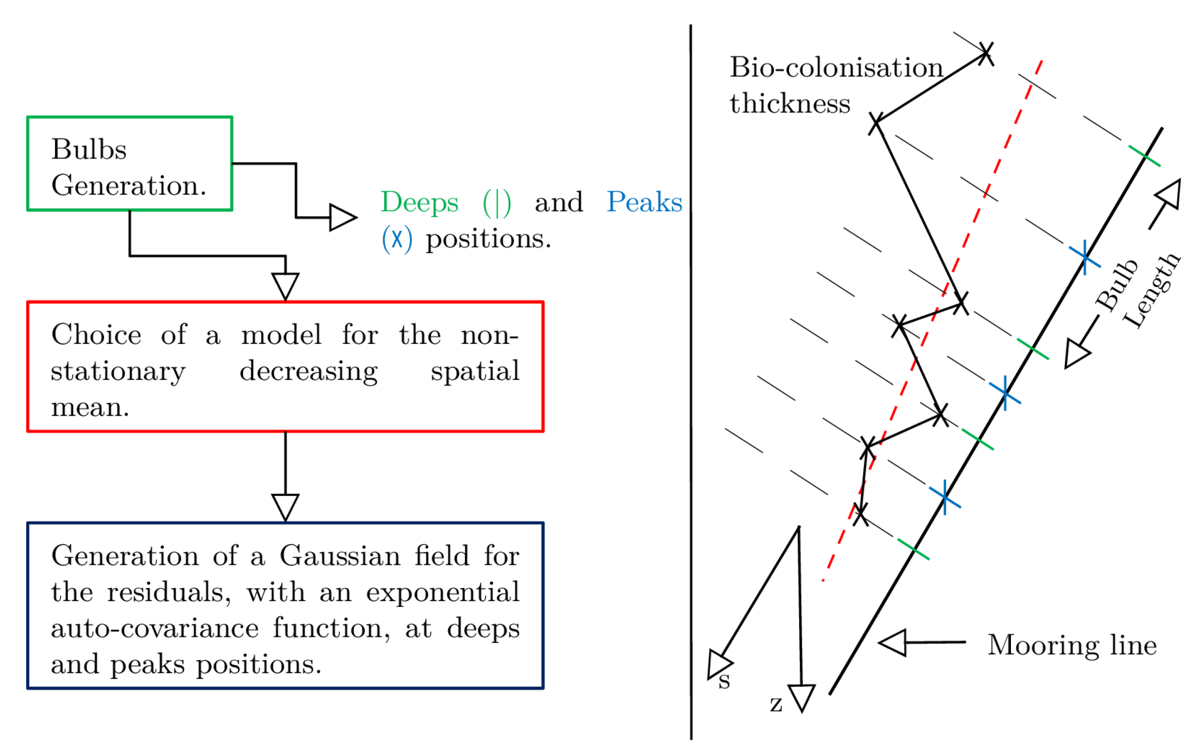
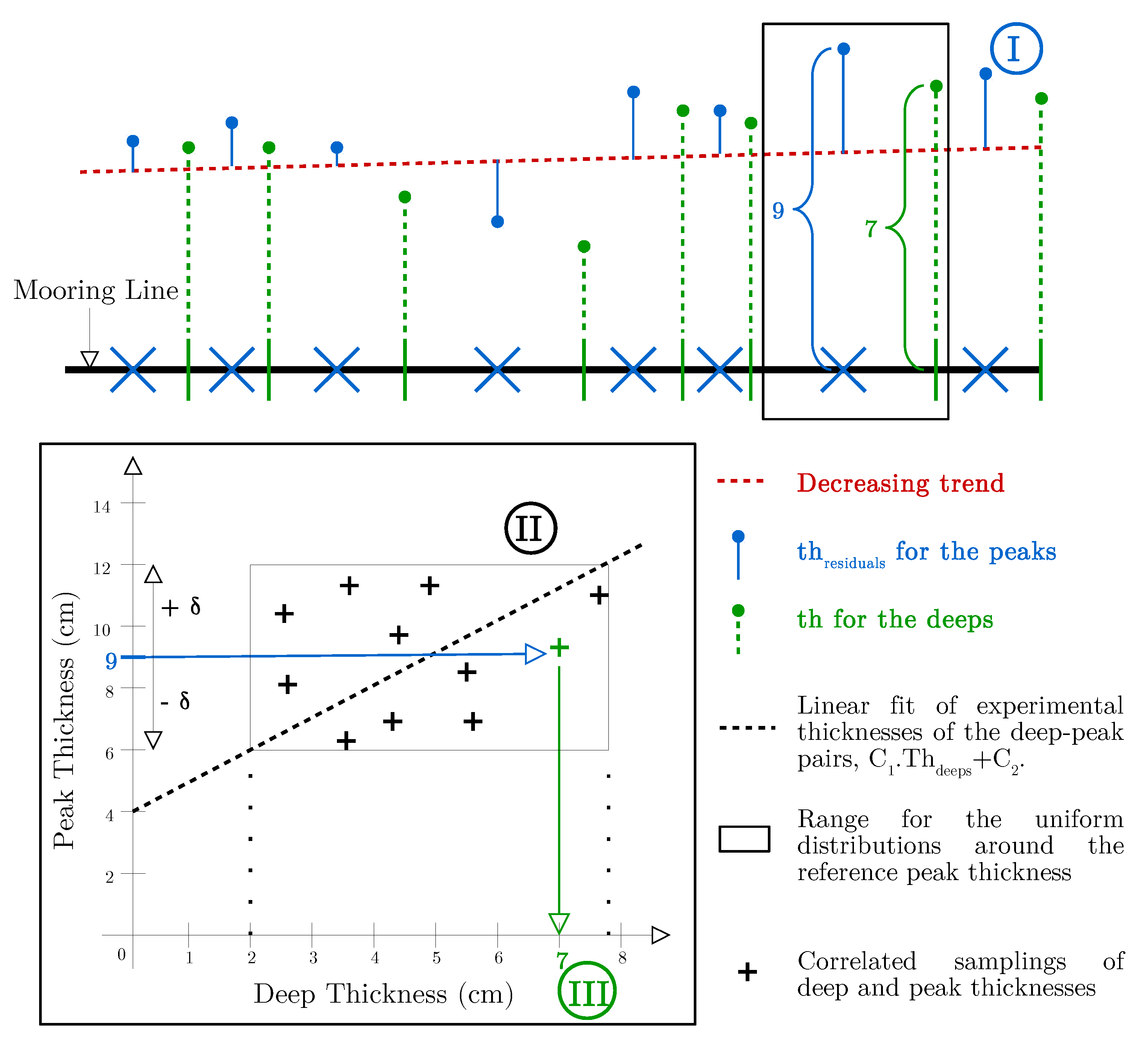
Appendix B. Generation of the Thicknesses for the Deeps

The above figure explains the generation of thicknesses for the deep positions (green graduation) depending on thicknesses for the peak positions (blue cross).
  • First (I), we generate a Gaussian field for the residuals at peak positions (blue), following Equation (2) but with μ r e s i d u a l s = 0.0195 m > 0 .
  • Second (II), for each peak thickness, now considered to be the reference value T h p e a k , r e f ( = 9 in Figure A5), we generate correlated samplings of deep and peak thicknesses from uniform distributions around the reference value, using a Gaussian copula and a correlation coefficient ρ D e e p / P e a k = 0.78083 . Peak thicknesses are uniformly sampled between T h p e a k δ and T h p e a k + δ . The upper and lower bounds for the sampling of deep thicknesses (doted lines) are respectively the antecedents of T h p e a k + δ and T h p e a k δ by the linear fit of experimental thicknesses of the deep-peak pairs (cf. Figure 9).
  • Third (III), we stop the generation of samplings when we find a sampling whose peak thickness T h p e a k , s a m p l i n g is close enough to the reference value ( | T h p e a k , r e f T h p e a k , s a m p l i n g | < 0.0005 m). The deep thickness of the selected sampling (7 in Figure A5) is then assigned to the deep position upstream the peak position of the reference peak thickness.
Please note that μ r e s i d u a l s for the peaks was calculated using the linear fit in order to obtain a null mean value of residuals when combining peaks and deeps. Therefore, μ r e s i d u a l s = C 2 ( C 1 + 1 ) .
Figure A5. Overview of the generation of thicknesses for the deep positions.
Jmse 08 00108 g0a5

Appendix C. Differential Entropy of a Truncated Normal Distribution

X Truncated normal Mean : μ ; Std : σ ; Min : t 1 ; Max : t 2 . Its probability density function f is then:
f ( x ; μ ; σ ; t 1 ; t 2 ) = ϕ x μ σ σ Φ t 2 μ σ Φ t 1 μ σ ; x t 1 ; t 2 , 0 ; x ; t 1 U t 2 ; + .
with ϕ , the pdf of the standard normal distribution and Φ , the cdf of the standard normal distribution. We now calculate the differential entropy H ( X ) :
H ( X ) + f ( x ) l n f ( x ) d x = t 1 t 2 f ( x ) l n f ( x ) d x .
So:
H ( X ) = t 1 t 2 f ( x ) l n 1 σ ϕ x μ σ d x + l n Φ t 2 μ σ Φ t 1 μ σ t 1 t 2 f ( x ) d x .
with: t 1 t 2 f ( x ) d x 1 and 1 σ ϕ x μ σ 1 2 π σ 2 e ( x μ ) 2 2 σ 2 .
From now to the end: T 1 = t 1 μ σ , T 2 = t 2 μ σ and C = Φ T 2 Φ T 1 . So:
H ( X ) = 1 C t 1 t 2 1 σ ϕ x μ σ l n 1 2 π σ 2 ( x μ ) 2 2 σ 2 d x + l n ( C ) .
= 1 C 1 2 l n 2 π σ 2 t 1 t 2 1 σ ϕ x μ σ d x 1 2 t 1 t 2 1 σ ϕ x μ σ x μ σ 2 d x + l n ( C ) .
with: t 1 t 2 1 σ ϕ x μ σ d x = Φ T 2 Φ T 1 = C and from now to the end: z = x μ σ . So:
H ( X ) = 1 C 1 2 l n 2 π σ 2 C 1 2 T 1 T 2 ϕ ( z ) z 2 d z + l n ( C ) .
with: T 1 T 2 ϕ ( z ) z 2 d z = 1 2 π T 1 · e T 1 2 2 T 2 · e T 2 2 2 + π 2 e r f T 2 2 e r f T 1 2 (calculated by using WolframAlpha). So finally we get:
H ( X ) = 1 2 l n 2 π σ 2 + 1 2 π T 1 · e T 1 2 2 T 2 · e T 2 2 2 + π 2 e r f T 2 2 e r f T 1 2 2 C + l n ( C ) .

References

  1. Fontaine, E.; Kilner, A.; Carra, C.; Washington, D.; Ma, K.; Phadke, A.; Laskowski, D.; Kusinski, G. Industry Survey of Past Failures, Pre-emptive Replacements and Reported Degradations for Mooring Systems of Floating Production Units. In Proceedings of the Offshore Technology Conference, Houston, TX, USA, 5–8 May 2014. [Google Scholar] [CrossRef]
  2. Pham, H.D.; Schoefs, F.; Cartraud, P.; Soulard, T.; Pham, H.H. Methodology for modeling and service life monitoring of mooring lines of floating wind turbines. Ocean Eng. 2019, 193. [Google Scholar] [CrossRef]
  3. Thies, P.R.; Johanning, L.; Harnois, V.; Smith, H.C.; Parish, D.N. Mooring line fatigue damage evaluation for floating marine energy converters: Field measurements and prediction. Renew. Energy 2014, 63, 133–144. [Google Scholar] [CrossRef] [Green Version]
  4. Ameryoun, H. Probabilistic Modeling of Wave Actions on Jacket Type Offshore Wind Turbines in Presence of Marine Growth. Ph.D. Thesis, Nantes University, Nantes, France, 2015. [Google Scholar]
  5. API. API RP 2A-WSD Recommended Practice for Planning, Designing and Constructing Fixed Offshore Platforms—Working Stress Design. 2005. Available online: http://latorebondeng90245.tripod.com/api_rp2a.pdf (accessed on 3 February 2020).
  6. DNVGL. DNVGL-OS-E301 Position Mooring. 2018. Available online: http://rules.dnvgl.com/docs/pdf/dnvgl/os/2018-07/dnvgl-os-e301.pdf (accessed on 5 February 2020).
  7. Wright, C.; Pakrashi, V.; Murphy, J. The Dynamic Effects of Marine Growth on a Tension Moored Floating Wind Turbine; Progress in Renewable Energies Offshore: Lisbon, Portugal, 2016. [Google Scholar] [CrossRef] [Green Version]
  8. Spraul, C.; Pham, H.D. Effect of Marine Growth on Floating Wind Turbines Mooring Lines Responses; AFM, Association Française de Mécanique: Lille, France, 2017. [Google Scholar]
  9. Yang, S.H.; Ringsberg, J.; Johnson, E. The Influence of Biofouling on Power Capture and the Fatigue Life of Mooring Lines and Power Cables Used in Wave Energy Converters; Progress in Renewable Energies Offshore: Lisbon, Portugal, 2016; pp. 711–722. [Google Scholar] [CrossRef]
  10. Spraul, C. Suivi en Service de la DuréE de vie des Ombilicaux Dynamiques pour L’éolien Flottant. Ph.D. Thesis, Ecole Centrale Nantes, Nantes, France, 2018. [Google Scholar]
  11. Jusoh, I.; Wolfram, J. Effects of Marine Growth and Hydrodynamic Loading on Offshore Strucutres. J. Mek. 1996, 1, 77–98. [Google Scholar]
  12. Boukinda Mbadinga, M.L.; Quiniou Ramus, V.; Schoefs, F. Marine Growth Colonization Process in Guinea Gulf: Data Analysis. J. Offshore Mech. Artic Eng. 2007. [Google Scholar] [CrossRef]
  13. O’Byrne, M.; Pakrashi, V.; Schoefs, F.; Ghosh, B. A Stereo-Matching Technique for Recovering 3D Information from Underwater Inspection Imagery. Comput. Aided Civ. Infrastruct. Eng. 2018, 33, 193–208. [Google Scholar] [CrossRef]
  14. Ameryoun, H.; Schoefs, F.; Barillé, L.; Thomas, Y. Stochastic Modeling of Forces on Jacket-Type Offshore Structures Colonized by Marine Growth. J. Mar. Sci. Eng. 2019, 7, 158. [Google Scholar] [CrossRef] [Green Version]
  15. Berhault, C.; Le Crom, I.; Le Bihan, G. SEM-REV: un moyen d’essais en mer multi-fonctions pour les énergies marines renouvelables. La Houille Blanche 2015, 2. [Google Scholar] [CrossRef]
  16. Qvarfordt, S.; Kautsky, H.; Malm, T. Development of Fouling Communities on Vertical Structures in the Baltic Sea. Estuar. Coast. Shelf Sci. 2006, 67, 618–628. [Google Scholar] [CrossRef]
  17. Relini, G.; Tixi, F.; Torchia, G. The Macrofouling on Offshore Platforms at Ravenna. Int. Biodeterior. Biodegrad. 1997, 41, 41–55. [Google Scholar] [CrossRef]
  18. Wilhelmsson, D.; Malm, T. Fouling Assemblages on Offshore Wind Power Plants and Adjacent Substrata. Estuar. Coast. Shelf Sci. 2008, 79, 459–466. [Google Scholar] [CrossRef]
  19. Compère, C.; Segonzac, M. Marine Growths on Offshore Structures; Technical Report; IFREMER: Plouzané, France, 2000.
  20. Parks, T.; Sell, D.; Picken, G. Marine Growth Assessment of Alwyn North A in 1994; Technical Report; Auris Environmental LTD: Aberdeen, Scotland, 1995. [Google Scholar]
  21. Clerc, R.; Oumouni, M.; Schoefs, F. SCAP-1D: A Spatial Correlation Assessment Procedure from unidimensional discrete data. Reliab. Eng. Syst. Saf. 2019, 191. [Google Scholar] [CrossRef]
  22. Burnham, K.P.; Anderson, D.R. Model Selection and Multimodel Inference—A Practical Information—Theoretic Approach; Springer: Berlin, Germany, 2002. [Google Scholar]
  23. Dietrich, C.R.; Newsam, G.N. Fast and Exact Simulation of Stationary Gaussian Processes Through Circulant Embedding of the Covariance Matrix. SIAM J. Sci. Comput. 1997, 18, 1088–1107. [Google Scholar] [CrossRef]
  24. Parks, T.; Cunningham, A.; Sell, D. Marine Growth on Alwyn North B in 1991; Technical Report; Auris Environmental LTD: Aberdeen, Scotland, 1991. [Google Scholar]
  25. Molin, B. Hydrodynamique des Structures Offshore; Guides Pratiques Sur Les Ouvrages en Mer; Editions TECHNIP: Paris, France, 2002. [Google Scholar]
  26. Malings, C.; Pozzi, M. Conditional entropy and value of information metrics for optimal sensing in infrastructure systems. Struct. Saf. 2016, 60, 77–90. [Google Scholar] [CrossRef]
  27. Verdugo, L.; Pushpa, N.R. On the Entropy of Continuous Probability Distributions. IEEE Trans. Inf. Theory 1978, 24, 120–122. [Google Scholar] [CrossRef]
  28. Györfi, L.; Beirlant, J.; Dudewicz, E.J.; van der Meulen, E.C. Non-Parametric Entropy Estimation: An Overview. Int. J. Math. Stat. Sci. 2001, 6, 17–39. [Google Scholar]
  29. Hall, P.; Morton, S.C. On the Estimation of Entropy. Ann. Inst. Stat. Math. 1993, 45, 69–88. [Google Scholar] [CrossRef]
Figure 1. Colonisation of mussels on the mooring chain of the Biocolmar buoy of Nantes University.
Jmse 08 00108 g001
Figure 2. Colonisation of uni-layered mussels on the mooring rope of a mussel farm.
Jmse 08 00108 g002
Figure 3. Definition of thickness (t) commonly used in standards vs. Practical measurement of thickness (th e x t ) on-site.
Jmse 08 00108 g003
Figure 4. Photograph of bio-colonisation on East cardinal buoy mooring chain of the SEMREV test site in February 2018.
Jmse 08 00108 g004
Figure 5. Trajectory of the bio-colonisation thickness on East cardinal buoy mooring chain in February 2018.
Jmse 08 00108 g005
Figure 6. Bulbs of mussels defined by alternating deeps and peaks.
Jmse 08 00108 g006
Figure 7. Frequency spectra calculated using an FFT algorithm.
Jmse 08 00108 g007
Figure 8. Diagram of the model with a scheme.
Jmse 08 00108 g008
Figure 9. Thicknesses of the deep-peak pairs.
Jmse 08 00108 g009
Figure 10. Normalised histograms of the length of bulbs.
Jmse 08 00108 g010
Figure 11. Comparison of three distributions to fit the experimental distribution of bulb lengths.
Jmse 08 00108 g011
Figure 12. Experimental covariogram of a dense sub-trajectory.
Jmse 08 00108 g012
Figure 13. Cross-section of a mussels cluster on a rope, revealing interstitial spaces.
Jmse 08 00108 g013
Figure 14. Density ρ o c p (kg·m 3 ) of mussels colonisation depending on its thickness.
Jmse 08 00108 g014
Figure 15. Mooring line of a FWT, monitored by four configurations of tension sensing network.
Jmse 08 00108 g015
Figure 16. Building samplings of posterior distributions of thickness and density parameters in calm sea state from tension measurements.
Jmse 08 00108 g016
Figure 17. Histograms of the conditional entropy metric for a, b and ρ (56 scenarii).
Jmse 08 00108 g017
Figure 18. Histograms of the conditional entropy metric for σ r e s i d u a l s and l c (56 scenarii).
Jmse 08 00108 g018
Figure 19. Histograms of the conditional entropy metric considering (a, b and ρ ) parameters depending on the number of sensors.
Jmse 08 00108 g019
Figure 20. Histograms of the conditional entropy metric considering only (a) parameter depending on the number of sensors.
Jmse 08 00108 g020
Table 1. LSE for a and b and their 95 % confidence bounds in brackets.
a (m)b
East Mooring before summer 2017 0.044 ; a [ 0.030 ; 0.059 ] 0.0010 ; b [ 0.002 ; 0 ]
West Mooring before summer 2017 0.036 ; a [ 0.018 ; 0.054 ] 0.0003 ; b [ 0.0016 ; 0.0009 ]
East Mooring in February 2018 0.082 ; a [ 0.069 ; 0.094 ] 0.0016 ; b [ 0.0030 ; 0.0002 ]
East Mooring in May 2018 0.140 ; a [ 0.113 ; 0.166 ] 0.0051 ; b [ 0.0074 ; 0.0029 ]
Table 2. Identification of σ r e s i d u a l s 2 and l c and their 95 % confidence bounds.
σ r e s i d u a l s 2 (m 2 ) l c (m)
East Mooring before summer 2017MLE 4.3 × 10 4 ; σ 2 [ 6.7 × 10 5 ; 7.9 × 10 4 ] 2.38 ; l c [ 0.20 ; 4.96 ]
West Mooring before summer 2017MLE 6.4 × 10 4 ; σ 2 [ 1.2 × 10 4 ; 1.2 × 10 3 ] 2.38 ; l c [ 0.16 ; 4.52 ]
East Mooring in February 2018LSE 2.1 × 10 3 ; σ 2 [ 2.0 × 10 3 ; 2.2 × 10 3 ] 1.24 ; l c [ 1.14 ; 1.33 ]
East Mooring in May 2018MLE 1.5 × 10 3 ; σ 2 [ 4.8 × 10 4 ; 3.5 × 10 3 ] 0.78 ; l c [ 0.29 ; 1.85 ]
Table 3. Definition of three different densities depending on interstitial and intervalvular waters.
Interstitial Water VolumeIntervalvular Water Mass
The “open porosity” density ( ρ o p )×
The “closed porosity” density ( ρ c p )×
The “open and closed” porosity density ( ρ o c p )
Table 4. Thickness and density parameters of each reference scenario of bio-colonisation.
Name of the Scenario a r e f (m) b r e f σ r e s i d u a l s , r e f (m) l c , r e f (m) ρ r e f (kg·m 3 )
Unfavourable site (US) 0.09 0.018 0.034 1.8 720
Favourable site after some months (FS) 0.04 0.0025 0.018 1.1 380
Full developed in favourable site (FD) 0.17 0.006 0.05 1.1 550
After a storm (AS) 0.035 0.0017 0.06 2 550
Table 5. Mass distribution of each reference scenario of bio-colonisation.
Name of the Scenario1 Sensor (kg)2 Sensors (kg)3 Sensors (kg)4 Sensors (kg)
Unfavourable site465 [ 465 ; 0 ] [ 465 ; 0 ; 0 ] [ 465 ; 0 ; 0 ; 0 ]
Favourable site after some months848 [ 848 ; 0 ] [ 795 ; 53 ; 0 ] [ 648 ; 200 ; 0 ; 0 ]
Full developed in favourable site 12,600 [ 10,375 ; 2225 ] [ 8184 ; 3594 ; 822 ] [ 6761 ; 3614 ; 1791 ; 434 ]
After a storm2863 [ 2863 ; 0 ] [ 1676 ; 1187 ; 0 ] [ 1512 ; 1351 ; 0 ; 0 ]
Table 6. Probabilistic distributions of the randomised parameters of bio-colonisation thickness.
Probabilistic Distribution
a (m)Uniform [ 0.01 ; 0.2 ]
bUniform [ 0.02 ; 0.0017 ]
σ r e s i d u a l s (m)Truncated normal (Mean: 0.034 m; Std: 0.013 m; σ m a x = 0.06 m; σ m i n = 0.008 m)
l c (m)Truncated normal (Mean: 1.1 m; Std: 0.45 m; l c , m a x = 2 m; l c , m i n = 0.2 m)
ρ (kg·m 3 )Uniform [ 300 ; 800 ]
Table 7. Differential entropy of uniform and truncated normal distributions.
Differential Entropy in NatsSource
X Uniform U 1 ; U 2 H ( X ) = l n U 2 U 1 [27]
X
Truncated normal
Mean : μ ; Std : σ ;
Min : t 1 ; Max : t 2
H ( X ) = 1 2 l n 2 π σ 2 +
1 2 π T 1 e T 1 2 2 T 2 e T 2 2 2 + π 2 e r f T 2 2 e r f T 1 2 2 Φ T 2 Φ T 1 +
l n Φ T 2 Φ T 1
Appendix C
Table 8. Excluded scenarii from analysis due to a low size of posterior sampling.
Reference Mass DistributionNumber of SensorsRelative Error Δ of Tension Measurement ( % )
Favourable site after some months45
Full developed in favourable site3
4
5
5
After a storm3
3
4
4
4
5
10
5
10
15
Table 9. Student’s t-test: the alternative hypothesis ( h = 1 ) is that the mean of the metric is greater than 0.
ab σ r e s i d u a l s l c ρ
h11001
p-value 2.25 × 10 22 5.30 × 10 7 9.99 × 10 1 9.71 × 10 1 5.2 × 10 3
Table 10. Does posterior sampling converge to reference value?
Nb Sensorsab ρ
123412341234
US Δ = 5 % ××××
Δ = 10 % ××××
Δ = 15 % ×××××
Δ = 20 % ×××××
FS Δ = 5 % ×××
Δ = 10 % ×××
Δ = 15 % ×××
Δ = 20 % ×××
FD Δ = 5 % Reference value
Δ = 10 %
Δ = 15 %
Δ = 20 % Prior mean =
AS Δ = 5 % ××××Reference value
Δ = 10 % ××××
Δ = 15 % ××××
Δ = 20 % ××××Prior mean =
Table 11. Correlation between metrics for a and inputs of scenarii.
Colonisation CaseNumber of SensorsError of Measurement ( Δ )
PearsonCorr = 0.0067
p-value = 0.9608
Corr = 0.5797
p-value = 2.8381 × 10 6
Corr = 0.1205
p-value = 0.3765
SpearmanCorr = 0.0274
p-value = 0.8411
Corr = 0.5695
p-value = 4.64 × 10 6
Corr = 0.0435
p-value = 0.7503
Table 12. Correlation between metrics for b and inputs of scenarii.
Colonisation CaseNumber of SensorsError of Measurement ( Δ )
PearsonCorr = 0.4352
p-value = 8.0251 × 10 6
Corr = 0.3970
p-value = 0.0025
Corr = 0.1774
p-value = 0.1908
SpearmanCorr = 0.4026
p-value = 0.0021
Corr = 0.2045
p-value = 0.1305
Corr = 0.2626
p-value = 0.0506
Table 13. Correlation between metrics for ρ and inputs of scenarii.
Colonisation CaseNumber of SensorsError of Measurement ( Δ )
PearsonCorr = 0.0032
p-value = 0.9814
Corr = 0.4114
p-value = 0.0016
Corr = 0.0728
p-value = 0.5939
SpearmanCorr = 0.0384
p-value = 0.7790
Corr = 0.2057
p-value = 0.1283
Corr = 0.2944
p-value = 0.0276

