Abstract
Knowledge of carbon and nitrogen isotopic ratios in organic matter and their changes is important when studying nutrient cycles in aquatic ecosystems. Relationships between δ13C and δ15N values of suspended particulate organic matter (POM), water temperature, salinity, pH, redox potential, chlorophyll a concentration, primary production, and biomasses of different taxonomic groups of phytoplankton in the Neva Estuary were statistically analyzed. We tested the hypothesis that the studied physicochemical and biogeochemical characteristics, as well as the species composition of phytoplankton and its productivity, can be significant predictors of changes in the isotopic ratios of suspended particulate organic matter in estuaries. In the Neva Estuary, δ13CPOM (−16.8–−27.6‰) and δ15NPOM (2.3–7.3‰) changed synchronously. Statistical analysis showed that for both isotopes, the photosynthetic activity and taxonomic composition of phytoplankton are important. For 13CPOM, the second most important factor was water salinity, which was apparently associated with the transition of algae from CO2 to HCO3 consumption during photosynthesis in estuarine waters. For 15NPOM changes, the most important abiotic factor was pH. The study showed that the dependences of POM isotopic ratios on environmental variables obtained for continental and oceanic waters are also valid in transitional zones such as the Neva Estuary.
1. Introduction
Stable isotope analysis is a standard technique for tracking organic matter transport and trophic interactions in both terrestrial and aquatic food webs [1]. The study of the isotopic composition of aquatic primary producers and its variability depending on abiotic environmental factors and taxonomic affiliation of primary producers in aquatic ecosystems is the key to understanding the cycle of autochthonous organic matter in water bodies [2]. A number of studies are devoted to the difference in the isotopic composition of phytoplankton, macroalgae, mangrove forests, and coastal swamps [2,3,4,5,6,7,8,9]. The important role of phytoplankton in the cycles of stable nitrogen isotopes in subtropical freshwater reservoirs and carbon in subtropical estuaries has been shown [10,11].
It is known that the carbon isotope ratios 13C/12C or “isotopic signature” expressed using the delta notation (δ13C) of organic matter of continental and marine origin is different. The largest active pool in the global carbon cycle is dissolved inorganic carbon (∑ DIC) in the oceans. This pool is mainly composed of HCO3− (≈95% carbon in ∑ DIC), but also includes dissolved CO2 (<1% of carbon) and CO3= (≈5% of carbon). The 13C/12C isotope ratio in the ∑ DIC ocean pool depends on the atmospheric CO2 input and the concentration of marine carbonates. Atmospheric CO2 has an intermediate concentration of 13C and averages δ13C = −7.8‰ in areas without large settlements and industrial production and −9.9‰ in urbanized areas [12]. In continental waters, the concentration of 13C in DIC depends on the ratio of dissolved atmospheric CO2, emission of carbon dioxide during the dissolution of rock carbonates, and CO2 release during the mineralization of soil organic matter coming from the catchment [12]. The isotopic ratio of rock carbonates, depending on the composition, varies from +2‰ in carbonate-rich to −12‰ in carbonate-poor soils.
The carbon isotope signature (δ13C) of organic matter coming from the catchment strongly depends on the prevailing type of photosynthesis in its vegetation [13]. The organic matter of plants with the C3 pathway of photosynthesis has an average δ13C value of about −27‰. Values for C4 plants range from −17 to −9‰, with a mean of −13‰, and plants with crassulacean acid metabolism (CAM) (mainly succulents of desert areas) on average have −19‰ [12]. The photosynthesis of phytoplankton occurs along the C3 pathway. However, the δ13C values of photosynthetic organisms in the ocean do not always resemble the δ13C values of terrestrial C3 plants, since marine phytoplankton can use bicarbonate as a carbon source for photosynthesis, the concentration of 13C in which is much higher than in the atmospheric CO2 ≈ 0‰ [12]. The mean δ13C values of marine, riverine, and lacustrine phytoplankton are close to −22‰, −27.5‰, and −34‰, respectively [12].
The factors that determine the δ15N and δ13C values of many phytoplankton species have been studied using pure algal cultures in the laboratory [4,14,15,16]. Laboratory culture experiments have shown wide fluctuations in the values of nitrogen and carbon isotope ratios (δ15N and δ13C) in various algal species and in their isotope fractionation factors. They can be used as indicators of 15N-enrichment and the assimilation of dissolved inorganic nitrogen by phytoplankton and the usage of carbon and nitrogen of different origin and in aquatic food webs. Although these studies have reported that the isotope ratios of suspended particulate organic matter (POM) can vary greatly over production cycles, little is known about the factors that determine its δ15N and δ13C values in natural systems.
It is assumed that in eutrophic waters, when intense photosynthesis leads to a lack of CO2, algae begin to consume carbon from the air, where the 13C content is higher than in water. As a result, the concentration of 13C in suspended particulate organic matter increases [17]. In addition, the taxonomic composition of phytoplankton influences the fractionation of 13C/12C [4,18,19]. For example, it was shown that a high proportion of dinoflagellates in marine phytoplankton near the coast of Portugal was accompanied by an increase in δ13C values [20]. On the contrary, an increase in the proportion of diatoms in the phytoplankton of the Mediterranean Sea led to a decrease in the 13C concentration in plankton [21].
The concentration of 15N isotope in aquatic ecosystems is closely related to the nitrogen cycle. The isotopic signature of phytoplankton nitrogen (δ15N) makes it possible to trace the nitrogen cycle in an aquatic ecosystem in order to determine the source and the predominant form of nitrogen compounds that phytoplankton consume [22,23]. The main nitrogen pool consists of nitrogen of organic matter and three mineral forms: ammonia form of nitrogen, nitrate form, and gaseous nitrogen [1]. In aquatic ecosystems, the processes that control the ratio of these forms are closely related to the microbial processes of nitrification and denitrification as well as nitrogen fixation [24]. Therefore, there is a clear need for further investigation of the factors that determine the δ15N and δ13C values of phytoplankton and suspended particulate organic matter in natural systems.
The Neva Estuary is the largest in the Baltic region, and the Neva River is the major contributor of freshwater to the sea [25]. The influx of nutrients into the estuary is significant due to the huge catchment area of the river and the location on the estuary coast of a large metropolis of St. Petersburg (5 million inhabitants), which discharges treated and untreated wastewaters into the estuary [26]. It currently receives 4630 tons of phosphorus and 57,000 tons of nitrogen annually, which is 8% of the nutrient load in the Baltic Sea from river runoff [27]. As a result, the primary productivity and biomass of planktonic autotrophic organisms in the estuary are among the highest in the Baltic Sea [8,28]. Recently, eutrophication has been increasing due to unfavorable weather conditions leading to an increase in the production of autochthonous organic matter in the estuary, which is not completely mineralized in the estuary waters and is carried further into the central part of the Gulf of Finland [29]. The phytoplankton of the estuary includes marine and freshwater species, the composition of which differs depending on environmental factors [30]. The isotopic ratios of suspended particulate organic matter, depending on the taxonomic composition of phytoplankton in the estuary, has not been studied previously, although this may be important for understanding the cycle of autochthonous and allochthonous organic matter not only in the Neva Estuary, but also in other estuaries with significant river runoff.
The study aims to determine carbon and nitrogen isotope ratios in suspended particulate organic matter depending on the abiotic and biotic characteristics of the aquatic environment. We tested the hypothesis that the physicochemical and biogeochemical characteristics of waters, as well as the species composition of phytoplankton and its productivity, can be significant predictors of changes in the isotopic ratios of suspended particulate organic matter in estuaries.
2. Materials and Methods
The Neva Estuary receives water from the Neva River, which is a relatively short canal (74 km) between Lake Ladoga and the Gulf of Finland, whose catchment area exceeds 280,000 km2, and the water discharge averages 2490 m3 s−1 (78.6 km3 yr−1), which is about one-fifth of the total river discharge into the Baltic Sea. The type of climate of the Neva Estuary region, according to Köppen–Geiger [31] climate classification, is Dfc (Snow climate, fully humid, cool summer). Soils on the estuary watershed according to Digital Soil Map of the World [32] are different types of Podzols in the northern part and different types of Podzoluvisol in the southern part, which are characterized by low pH and a low concentration or absence of carbonates. The Neva Estuary is brackish-water, non-tidal, with horizontal and vertical gradients of salinity and dominance of eurytopic species. The upper part of the estuary was separated from its lower part by the Flood Protective Facility (Dam). It consists of eleven dams separated by broad water passages and ship gates in its southern and northern parts (Figure 1). Due to the low transparency of the water, most of the estuary is free of bottom vegetation. Dense reeds of 300–600 m width belt only its shallow coastal zone. A more detailed description of the estuary was given in previous publications [8,29].
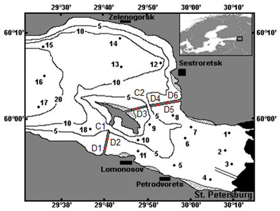
Figure 1.
The Neva Estuary with an indication of the sampling stations. Black lines show 5, 10, and 20 m isobaths. Areas with dots indicate dense reeds. C1, C2—gates for vessels; D1–D6—waters gates in the St. Petersburg Flood Protection Facility.
2.1. Sampling
Eighteen stations in the Neva Estuary (Figure 1) were sampled twice: from 20th of July to 5th of August in 2018 and 2019. The temperature, salinity, and redox potential (ORP) were determined at each station using a CTD90m probe (Sea&Sun Tech., Trappenkamp, Germany) every 20 cm from the surface to the bottom. Taking into account that according to these measurements, the whole water column in the shallow upper part was mixed, we collected five water samples (2 L each): from the surface, half a meter from the bottom, and from three equal depths between them. Samples from different depths were taken in order to avoid errors associated with the vertical distribution of different phytoplankton species in the water column. These samples were mixed to make up a composite sample (10 L). Samples (three replicates of water collection) of chlorophyll a, suspended particulate organic matter, and stable isotope analysis (SIA) were taken from these composite samples.
At the stations 12–18, where temperature stratification was observed, composite water samples were taken from the layer above (UL) the thermocline. Five water samples (2 L each) were taken from the UL: from the surface, the thermocline, and from three equal depths between them. These samples were mixed to create a composite sample (10 L). The samples of chlorophyll a, suspended particulate organic matter, and samples for stable isotope analysis (three replicates of water collection) were taken from these composite samples.
2.2. Laboratory Analysis
Three hundred milliliters of water were filtered through 0.85 µm membrane filters (Millipore AAWP, Burlington, MA, USA) to determine the chlorophyll a (Chl a) concentration, which was followed by 90% acetone extraction and spectrophotometric determination [33]. Suspended particulate organic matter (POM) was determined after filtration (Whatman GF/F filters, Maidstone, UK) with the dichromate acid oxidation [33].
The primary production of plankton (PP) in the water column were measured by the oxygen method of light and dark bottles [34,35]. A more detailed description of the method and experimental design is given in Golubkov et al. [8].
For SIA, one liter of composite water sample passed through a 50 µm mesh to separate zooplankton and coarse particles were filtered through pre-combusted Whatmann GF/F 0.7 µm glass fiber filters to collect POM, which consisted mainly of estuarine phytoplankton, with an admixture of riverine phytoplankton, detritus, and terrigenous (with wastewater) POM. POM samples for SIA were frozen at −20 °C until analysis of stable isotope ratios. Before analysis, filters with POM were dried at 60 °C for 48 h. After drying, samples were homogenized in an agate mortar to make a composite sample. Analyses were performed on POM homogenized composite samples desiccated for 24 h in a desiccator. Triplicate POM composite samples (1.0–1.3 mg) were put into small tin capsules and weighed using a Mettler Toledo MX 5 balance with an accuracy of ±1 μg. The SIA was performed according to standard methods [36] using a Thermo Delta V Plus isotope mass spectrometer (Thermo Scientific, Waltham, MA, USA) equipped with an element analyzer at the Joint Usage Center «Instrumental methods in ecology» of A.N. Severtsov Institute of Ecology and Evolution of RAS (Moscow, Russia, Russian Federation). An isotopic composition of C and N in organic matter was expressed in δ-notation relative to international standard (vPDB for carbon and the atmospheric N2 for nitrogen) δ (‰) = (Rsample/Rstandard − 1) × 1000, where R= 13C/12C or 15N/14N. Samples were analyzed with reference gas calibrated against IAEA (Vienna, Austria) reference materials USGS 40 and USGS 41. The drift was corrected using an internal laboratory standard (casein). The standard deviation of δ13C and δ15N values in the laboratory standard (n = 8) was <0.2‰.
2.3. Phytoplankton Assemblages
Phytoplankton (volume 0.3 L) was taken in one replicate from a composite sample and fixed with acid Lugol’s solution. The phytoplankton taxa were identified and counted in sedimentation chambers (10–25 mL) with an inverted Hydro-Bios microscope. Phytoplankton biomass was calculated in total volume of algal cells according to Olenina et al. [37]. The biomasses for each species from the same taxonomic group were summarized and used in statistical analysis.
2.4. Statistical Analysis
Statistical analyses were performed using R software (version 3.6.0) [38]. The Pearson correlation coefficients matrix was produced using the “table.correlation” function in the PerformanceAnalytics R package [39]. Stepwise multiple linear regressions were performed to determine the most influential factors affecting δ13C and δ15N in POM. We have built “model.null” separately for δ13C and δ15N and “model.full” with all environmental factors, the taxonomic composition of phytoplankton and separately for δ13C and δ15N in POM. As a result, two models (null and full) were done for δ13C and two were done for δ15N. Then, the “step” function (direction = "both") was used to add and remove factors from the model and to find the model with the lowest Akaike Information Criterion (AIC). AIC was used as an estimator of out-of-sample prediction error and thereby the relative quality of statistical models for a given set of data. The lower the value, the better for the AIC [40]. When the model with the lowest AIC was found, it was called the final.model. This procedure was done separately for δ13C and δ15N in POM, and two final.models for δ13CPOM and δ15NPOM were chosen and combinations of the most influential factors were found separately for δ13CPOM and δ15NPOM. Afterwards, we did an analysis of variance for individual factors included in the final models by the function “Anova” in the car R package [41] to determine which one is most important for the prediction of δ13CPOM and δ15NPOM in each final model. The residuals plots were checked for two final models, and it showed that residuals were unbiased and homoscedastic. A stepwise multiple linear regressions analysis is detailed in Mangiafico [40].
3. Results
3.1. 13CPOM and 15NPOM Ratios and Environmental Variables
The water temperature in the Neva Estuary during the sampling period varied from 18 to 24 °C. Data on water temperature in this range were evenly distributed over the entire set of values, since the mean and median practically coincided (Table 1). Salinity ranged from 0.08 to 2.81, with an average of 0.71 PSU, but a median of 0.14 PSU. This means that most of the water sampling sites were in slightly saline waters. The pH values were biased to the alkaline range from 7.8 to 10 and were almost evenly distributed across all stations. The ORP values varied in the range 148–312 mV, showing the presence of free electrons in the solution and the ability of the latter to take or donate electrons to chemical compounds contained in it.

Table 1.
Number of samples (no.), maximum, minimum, median, interquartile range (IQR), average and standard deviation (SD) of environmental variables and δ13CPOM and δ15NPOM values in the Neva Estuary during the study period. S-water salinity; T-water temperature; ORP-RedOx potential; POM—concentration of suspended particulate organic matter; Chl a—concentration of chlorophyll a; PP—primary production of plankton.
The concentration of suspended particulate organic matter ranged from 0.9 to 4.9 g m−3 and chlorophyll a ranged from 5.6 to 98.1 mg m−3 (Table 1). The primary production of plankton changed during the study period by a factor of ten, depending on the station (from 0.31 to 3.96 gC m−2 d−1). δ13CPOM in the estuary varied from −16.8 to −27.6‰ (averaging about −25‰), δ15NPOM varied from 2.3 to 7.3‰ (averaging about 4.8‰) (Table 1). Average values of δ13CPOM and δ15NPOM in the Neva River waters were −26.8‰ and 0.9‰, consequently [26].
3.2. Taxonomic Composition of Phytoplankton
Eighty-nine phytoplankton species belonging to seven taxonomic groups were found in the investigated part of the estuary during the study period (Table 2). Most of the species (36) belonged to green algae, while in second place in terms of species richness were cyanobacteria (19 species), and in third place were diatoms (16 species). The other four taxonomic groups included only from three to six species (Table 2). Nevertheless, the algae of these species-poor groups often had the highest biomasses. For example, the highest biomass recorded at one sampling station belonged to cryptophytic algae, with dinoflagellates in second place. However, if cryptophytic algae had both the highest median and mean biomasses for all stations, then this was not the case for dinoflagellates (Table 2). Green algae and diatoms were the first in frequency of occurrence; Euglenophyceae were the rarest of the seven taxonomic groups (Table 2).
Table 2.
Number of species and occurrence, maximum, minimum, median, and mean biomass (wet weight mg m−3), interquartile range (IQR), and standard deviation (SD) of each taxonomic group in phytoplankton assemblages in the Neva Estuary in midsummer 2018–2019.
Cryptophyceae accounted for the bulk (24%) and Bacillariophyceae played a significant role in the total biomass of phytoplankton (Figure 2). These two groups together accounted for 45% of the phytoplankton biomass. Cyanophyceae and Euglenophyceae were next in biomass, and Chrysophyceae had the lowest biomass (Figure 2).
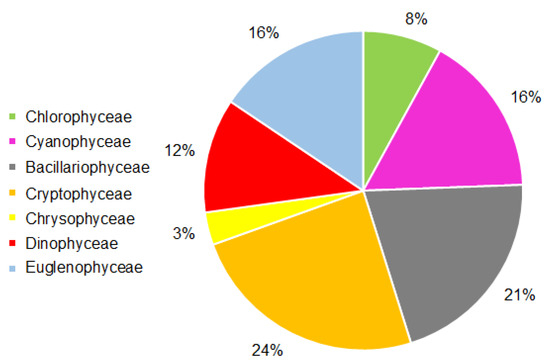
Figure 2.
The contribution of various taxonomic groups to the total biomass of phytoplankton in the Neva Estuary in midsummer 2018–2019.
3.3. Relationship between 13CPOM and 15NPOM Ratios, Environmental Variables, and Taxonomic Composition of Phytoplankton
The analysis of the data, carried out by the Pearson’s pair correlation method, showed that all the studied parameters are quite closely interrelated with each other. Values of δ13CPOM significantly correlated with all the studied environmental variables (Figure 3). However, the strength of the statistical relationship and the level of confidence were different. The highest and most reliable positive correlation coefficients were obtained between δ13C values and phytoplankton productivity indicators: chlorophyll a concentration and primary production of plankton. Slightly weaker statistical relationships were obtained between this isotope ratio, POM and pH. This was most likely due to the correlations of these variables with chlorophyll a and primary production (Figure 3). The close correlation of the POM concentration with the Chl a concentration suggests that phytoplankton constituted the bulk of suspended particulate organic matter, and its active photosynthesis led to an increase in pH values and a shift of this indicator to a more alkaline range.
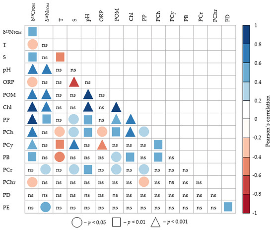
Figure 3.
Pearson’s correlation coefficients between δ13CPOM and δ15NPOM values of suspended particulate organic matter, environmental variables, biomasses of Chlorophyceae (PCh), Cyanophyceae (PCy), Bacillariophyceae (PB), Cryptophyceae (PCr), Chrysophyceae (PChr), Dynophyceae (PD) and Euglenophyceae (PE) in the Neva Estuary in midsummer 2018–2019. Abbreviations of environmental variables are the same as in Table 1.
Water salinity positively correlated with δ13CPOM values and did not correlate with the chlorophyll a concentration. δ13CPOM values also weakly negatively correlated with water temperature and ORP (Figure 3)
In general, δ15NPOM and δ13CPOM values were positively significantly correlated with each other (Figure 4). However, the δ15NPOM values correlated somewhat differently with the other studied variables. Of the environmental variables studied, δ15NPOM values most closely correlated with pH. This isotope ratio also showed a significant positive relationship with biotic environmental factors, but the relationship was weaker compared to δ13CPOM. At the same time, in contrast to δ13CPOM, the δ15NPOM values did not show any relationships with water temperature, salinity, and ORP values (Figure 3).
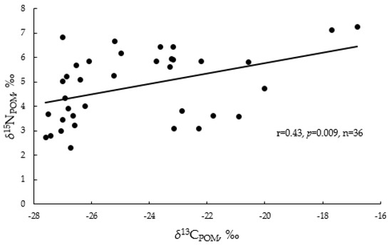
Figure 4.
Linear regression between δ13C and δ15N in suspended particulate organic matter (POM) in the Neva Estuary in midsummer 2018–2019.
The pairwise correlation method showed that the carbon isotope ratio in suspended particulate organic matter significantly positively correlated with the biomasses of three groups of phytoplankton and negatively correlated with the biomass of one group. The δ13CPOM values were most significantly correlated with the biomasses of Chlorophyceae and Cyanophyceae, and the correlation coefficient with the first group was higher (Figure 3). The positive relationship between δ13CPOM values and Bacillariophyceae biomass was slightly weaker. In total, these three groups of phytoplankton accounted for 45% of the total phytoplankton biomass. Moreover, these groups had the highest biomasses at the same stations, as evidenced by the positive significant correlations between their biomasses. The δ13CPOM values negatively correlated with the biomass of Chrysophyceae, which had the smallest proportion in the phytoplankton biomass. No significant relationship was found between the carbon isotope ratio and biomasses of the other three groups of algae (Figure 3).
The δ15NPOM values practically did not correlate with the biomasses of various groups of algae. Only two groups of algae showed a weak positive relationship with δ15NPOM values (Figure 3). We also tried to carry out a correlation analysis between δ15NPOM and δ13CPOM values and the biomass of certain phytoplankton species, but we did not get any significant correlations.
3.4. Stepwise Multiple Regression Analyses between Stable Isotope Ratios, Environmental Variables, and Phytoplankton Taxonomy Groups
Analysis by the method of pairwise correlations showed that the carbon and nitrogen isotope ratios correlate with the studied abiotic environmental factors and the biomasses of some taxonomic groups of phytoplankton. However, in nature, environmental factors often do not act separately from each other, but are intertwined in a complex system of interrelationships. To find out how these factors together can be associated with changes in the concentrations of carbon and nitrogen isotopes in suspended particulate organic matter, a stepwise multiple regression analysis was carried out. We conducted simulations and obtained two models, separately for δ13CPOM and δ15NPOM values, which best described the changes in these parameters in the estuary POM, taking into account the studied factors. According to plots of residuals vs. predicted values for δ13CPOM and δ15NPOM models (Figure 5), both models are unbiased and homoscedastic.
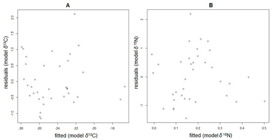
Figure 5.
Plots of residuals vs. predicted values for δ13CPOM (A) and δ15NPOM (B) models.
For the carbon isotope model, six of the fourteen indicators turned out to be predictors: chlorophyll a concentration, water salinity, plankton primary production, as well as biomasses of Cryptophyceae, Euglenophyceae, and Chlorophyceae. The coefficient of linear determination of the model was high (R2 = 0.93). However, in order to avoid the error of its overestimation, which occurs as a result of adding each additional predictor to the model, we calculated the adjusted R2 (Adj R2), and it also showed a high value of 0.92. This means that the resulting regression model was in good agreement with the observed values. This is also evidenced by the high level of significance (p-value) of the model—7.56 × 10⁻¹⁶, i.e., the chances of obtaining a reliable result with this model were very high.
Three predictors that were obtained had a positive relationship with the δ13C values of POM, and the relationship of the other three was negative. The combined increase in salinity, chlorophyll a, and primary production of plankton led to an increase in the concentration of the carbon isotope. On the contrary, an increase in the biomasses of Cryptophyceae, Euglenophyceae, and Chlorophyceae led to its decrease, i.e., they acted as negative predictors.
The resulting regression equation describing the change in δ13CPOM values in the Neva Estuary depending on significant environmental factors is given in Table 3. To find out the significance of the predictors and which of them most strongly influenced the 13C concentration in POM, we carried out the t-test and F-test and found that the most significant predictors in the δ13CPOM models were the chlorophyll a concentration and water salinity. Their t-value and F-value were the highest. Consequently, it was the changes in chlorophyll a concentration and water salinity that most strongly influenced the changes in δ13CPOM values. Chlorophyll a concentration and water salinity variables did not correlate with each other (Figure 3), so there was no multicollinearity problem in the model. For the δ13CPOM value to increase by 1‰, the salinity of the water had to increase by 1.56 PSU, the chlorophyll a concentration had to increase by 0.14 mg m−3, and plankton primary production had to increase by 0.49 gC m-2day-1. Although the values of plankton primary production had a positive effect on the increase in δ13C values in the model, they did not play a major role in the increase in the isotope concentration, as evidenced by the low t-value and F-value, as well as the p-value. They were significant only in combination with other predictors but not by themselves.
Table 3.
Results of the stepwise multiple regression analyses between δ13C values of suspended particulate organic matter (Y variable), environmental variables, and biomasses of various phytoplankton groups (X variables). Abbreviations of environmental variables and phytoplankton groups are the same as in Table 1 and Table 4.
The algal biomass was found to be a negative predictor of the regression model. The most significant factor was the biomass of Euglenophyceae, followed by the biomass of Chlorophyceae. Although the biomass of Cryptophyceae improved the model, it itself had little effect on the final result, i.e., as well as primary production, it was important only together with other factors. A decrease in the biomass of Euglenophyceae by 0.10, Chlorophyceae by 0.28, and Cryptophyceae by 0.42 g m−3 wet weight led to an increase in the δ13C value of suspended particulate organic matter by 1‰ (Table 3).
For the δ15N model of suspended particulate organic matter, five of the fourteen studied indicators were found to be significant predictors. Of these, the values of pH, plankton primary production, and the biomass of Euglenophyceae turned out to be positive predictors, and the biomasses of Cyanophyceae and Chrysophyceae were negative predictors (Table 4).
Table 4.
Results of the stepwise multiple regression analyses between δ15N values of particulate organic matter (POM) (Y variable), environmental variables, and biomasses of various phytoplankton groups (X variables). Abbreviations of environmental variables and phytoplankton groups are the same as in Table 1 and Table 4.
Although the model for nitrogen was statistically significant, the coefficients of linear determination (R2) and adjusted R2 (Adj R2) were lower than for carbon, 0.63 and 0.57, respectively. The level of significance (p-value) of the model for the δ15N values of suspended particulate organic matter was also lower than for the δ13CPOM values, but it was still quite high (p-value = 8.08 × 10⁻⁶). The most significant predictors of the δ15NPOM model were the pH and biomass of Cyanophyceae; they had the highest t-value and F-value. However, an increase in pH had a positive effect on the δ15NPOM values, while the biomass of Cyanophyceae had a negative effect (Table 4). A decrease in the biomass of Chrysophyceae also had a significant negative effect on the δ15NPOM. The primary production and biomass of Euglenophyceae separately did not significantly affect the δ15NPOM values, but their addition to the regression model had a positive effect on the overall accuracy of the model. The obtained regression equation shows that to increase δ15N values of POM by 1‰, it is necessary for the pH to increase by 1.37, for the primary production to by 0.44 gCm−2day−1, and for the biomass of Euglenophyceae to increase by 0.05 g m−3. At the same time, the biomass of Cyanophyceae should decrease by 0.11 g m−3, and that of Chrysophyceae should decrease by 0.49 g m−3.
4. Discussion
4.1. Carbon Isotope Ratio in Suspended Particulate Organic Matter
According the results of this study, physicochemical and biogeochemical characteristics of waters, as well as the species composition of phytoplankton and its productivity, can be significant predictors of changes in the isotopic ratios of suspended particulate organic matter in estuaries. Analysis of pairwise correlations showed that its values had high significant positive correlations with the level of plankton primary production, chlorophyll a concentration, and water salinity.
It is well known that isotopic signature of organic matter of continental and marine origin is different [12]. In our study, the mean δ13C values of POM were about 25‰ (Table 2), which is in the middle between the values for marine and river phytoplankton. In the estuaries of North America with significant river runoff, the 13CPOM concentration increased with increasing water salinity, and this effect was observed in all seasons of the year [42]. In the Neva Estuary, we observed a similar trend. However, the carbon isotope signature in the Neva Estuary was also strongly correlated with plankton productivity (Figure 3). Moreover, multi-regression analysis of our data showed that for an increase in the concentration of stable carbon isotope in the suspended particulate organic matter of the Neva Estuary, a necessary condition was a simultaneous increase in the concentration of chlorophyll a and water salinity. This means that with active photosynthesis, as the salinity of water increased, plankton switch to the use of bicarbonates instead of CO2 as carbon sources, which occurs when CO2 dissolved in the water is exhausted during the mass development of algae, as was shown previously [4,43]. Our data show that at high levels of primary production in eutrophic waters, even a slight increase in salinity per 1 PSU leads to an increase in 13C concentration.
The water temperature showed a pairwise correlation with the δ13C values of suspended particulate organic matter (Figure 3), but it was not included in the number of significant environmental variables in the multi-regression model (Table 3). As was previously shown, the δ13C values of phytoplankton in the Atlantic Ocean correlate with water temperature, and this is associated not only with a change in the taxonomic composition of phytoplankton but also with the difference in its enzymatic activity depending on temperature [44]. This dependence was determined for the temperature range from −2 to +33 °C, but at the same time, the authors showed that above 18 and up to 33 °C, the value of δ13C practically does not change. During the period of our study, the water temperature was from 18 to 24 °C (Table 1). This apparently was the reason that we did not get a significant effect of temperature on the concentration of 13C in suspended particulate organic matter (Table 3). Therefore, the dependence obtained for oceanic waters is also valid for the Neva Estuary.
13C/12C fractionation varies depending on physiological characteristics and enzyme composition in phytoplankton [4,18,19,44]. This is well shown for marine phytoplankton consisting of dinoflagellates and diatoms [20,21]. In our study, the analysis of pairwise correlations showed that the δ13CPOM values increased synchronously with the increase in the biomasses of green algae, diatoms, and cyanobacteria (Figure 3). Multi-regression analysis showed that the biomass of algae of only three groups (Euglenophyceae, Chlorophyceae, and Cryptophyceae) significantly influenced the δ13CPOM values (Table 3). Moreover, the biomasses of algae of these groups acted as negative predictors of the model, i.e., an increase in their role in the phytoplankton community led to a decrease in δ13CPOM values. Therefore, in our opinion, the 13C concentration in the Neva Estuary is affected not only by the total amount of algae but also by the taxonomic composition of phytoplankton assemblages. However, based on the F-value, which varied from 2.4 to 4.2, one can conclude that the taxonomic composition of the phytoplankton community plays a smaller role in the change in δ13CPOM values of suspended particulate organic matter compared to the concentration of chlorophyll a and water salinity (F-test was 57.4 for chlorophyll a and 46.0 for salinity, p = 0.001).
4.2. Nitrogen Isotope Ratio in Suspended Particulate Organic Matter
Among environmental factors, δ15NPOM values in the Neva Estuary did not correlate with salinity, redox conditions, or temperature, but only with pH, chlorophyll a concentration, and the level of primary production (Figure 3). At higher values of these parameters, the concentration of 15N in POM was higher. However, these significant correlations may be indirect, because an analysis of pairwise correlations showed that the δ15NPOM values in the Neva Estuary changed synchronously with the δ13CPOM values; with an increase in the proportion of one isotope in suspended particulate organic matter, the proportion of the second one also increased (Figure 4). The same synchronous change is shown with an increase in the trophic status of freshwater ecosystems, and it is associated with biochemical and biogeochemical processes caused by the intensive development of phytoplankton [45].
Multi-regression analysis showed that pH was the main predictor of the model; its increase most of all increased the δ15NPOM values (according to the results of the F-test, F = 11.76, p = 0.018; Table 4). At the same time, the salinity of the water did not affect the pH value, as evidenced by the lack of correlation between these variables (Figure 3), apparently this was due to a slight change in this parameter in the current dataset (salinity median 0.14 PSU) (Table 1). It is important to take into account that the increase in pH in the Neva Estuary was apparently caused by the active photosynthesis of algae, since the concentration of Chl a and PP correlated significantly with the pH values. Moreover, it is known from the literature that the pH of water increases with active photosynthesis [46]. This result is interesting, since pH is not considered as the main factor influencing the δ15NPOM values, but it does not contradict the previously obtained results. For example, in a recent review and model study on the effect of ocean acidification on the nitrogen cycle, Wannicke et al. [47] showed that a decrease in water pH leads to a decrease in the rate of nitrification, and in this connection, the authors predict an essential increase in the proportion of ammonia nitrogen in the upper water layers. In turn, an increase in the concentration of ammonium nitrogen and low pH values shift the isotopic signature of nitrogen in the negative direction [45]. For instance, δ15N values of phytoplankton ranged from −7.8 to −3.4‰ in Japanese volcanic lake with the pH of about 2, and an increase in ammonia concentration statistically significantly negatively correlated with 15N concentration [48].
The taxonomic composition of phytoplankton also had less effect on δ15NPOM compared to δ13CPOM. Only the biomasses of Cryptophyceae and Euglenophyceae were significantly positively correlated with the nitrogen isotope ratio. According to multi-regression analysis, the second most important predictor was the biomass of cyanobacteria. An increase in the biomass of cyanobacteria led to a decrease in δ15NPOM values (Table 3 and Table 4). This is consistent with data on the isotopic signature of suspended particulate organic matter in lakes, for which it was shown that the isotope signature of nitrogen decreases to ≈0‰ when nitrogen-fixing bacteria dominate in the phytoplankton community [49]. The biomass of Chrysophyceae was also a significant negative predictor in our model. We could not find in the literature studies on the relationship between the isotopic composition of suspended particulate organic matter and Chrysophyceae, since this group is usually not considered as important or dangerous to humans. However, our research shows that these algae may play a role in the nitrogen cycle, and the study of this group would be useful for understanding the biogeochemical nitrogen cycle in aquatic ecosystems.
In our study, the primary production of plankton was a positive predictor of δ15NPOM values (Table 4), and the same result was obtained when analyzing Pearson’s pairwise correlations (Figure 3). Earlier, the analysis of data on 36 lakes with various morphometric and physicochemical characteristics, and trophic status from oligotrophic to hypereutrophic showed a similar trend [49]. It was found that the δ15N values of suspended particulate organic matter increased from oligotrophic to eutrophic lakes, but their values decreased in hypereutrophic lakes. The author concluded that this was due to the cyanobacteria, which dominated in hypereutrophic lakes, fixed nitrogen from the air and, as a result, reduced the 15N concentration in POM. According to our data, this is apparently also true for estuaries with a significant runoff of river waters, since the δ15N values of POM increased with an increase in PP and chlorophyll a concentration, and an increase in the proportion of Cyanophyceae in the total phytoplankton biomass led to a decrease in the δ15NPOM values.
An interesting result was obtained on the effect of Euglenophyceae on the isotopic ratios of nitrogen and carbon in POM in the Neva Estuary. Both the method of pairwise correlations and multi-regression analysis showed that with an increase in their biomass, the values of δ15NPOM increased, while the δ13CPOM values decreased. This may be due to the fact that these organisms are equally capable of both photosynthesis and phagotrophy [50]. As a source of nutrients, Euglenophyceae can consume bacteria and other protozoa, as well as POM entering the Neva Estuary with wastewater and thereby increase the 15N pool and reduce the 13C pool, since wastewater is characterized by high nitrogen and relatively low carbon isotope ratios [12,26,45,51]. In addition, some Euglenophyceae are able to feed on cyanobacteria [52], the increase in biomass of which led to a decrease in 15N in POM of the Neva Estuary. However, a special study is required to clarify this issue.
Analysis of pairwise correlations also showed that the biomass of Cryptophyceae in the Neva Estuary was positively correlated with δ15NPOM. As with Euglenophyceae, these algae can switch to heterotrophic nutrition and consume suspended particulate organic matter [53,54]. Perhaps this is the reason why they can increase the 15N pool in the Neva Estuary. However, this requires additional research.
5. Conclusions
The study showed that the concentrations of 13C and 15N change synchronously in suspended particulate organic matter of the Neva Estuary; with an increase in one, the other also increases. This suggests that the nature of their accumulation in the suspended particulate organic matter in the estuary is closely related to the processes of production of organic matter by phytoplankton. Pairwise correlations and multi-regression showed that for both isotopes, and especially for δ13CPOM values, the photosynthetic activity of algae is important, the indicator of which is the concentration of chlorophyll a and the level of plankton primary production. However, statistical analysis showed that for δ13CPOM values, the second most important factor is water salinity, which is apparently associated with the transition of algae during active photosynthesis from CO2 consumption to HCO3. For δ15NPOM values, the most important abiotic factor was pH, the fluctuations of which were associated with the photosynthetic activity of plankton. The change in pH apparently affects the microbiological activity in the water column, which affects the nitrogen cycle in water and the predominance of certain mineral forms (NH4, NO3, etc.) that algae consume as a source of nitrogen. The analysis showed that the taxonomic composition of phytoplankton also influenced the concentrations of 13C and 15N isotopes in suspended particulate organic matter. The biomasses of certain taxonomic groups of phytoplankton acted as additional predictors of multiregression models for 13C and 15N changes in suspended particulate organic matter in the Neva Estuary. However, additional research is required, especially on the effect on the isotope signature of Euglenophyceae and Cryptophyceae, which are capable of heterotrophic feeding. In addition, it can be concluded that the dependences (the influence of trophic status, salinity, temperature, pH on isotopic ratios in POM) obtained for continental freshwaters and oceanic waters are also valid in transitional zones, such as the Neva Estuary.
Author Contributions
Conceptualization, M.S.G.; field sampling M.S.G., and S.M.G.; laboratory analyses M.S.G., V.N.N., and A.V.T.; analyzed the data, M.S.G.; visualization, M.S.G.; writing—original draft preparation, M.S.G., S.M.G., and A.V.T.; writing—review and editing, M.S.G., and S.M.G.; project administration, S.M.G.; funding acquisition, S.M.G. All authors have read and agreed to the published version of the manuscript.
Funding
The study was supported by the Ministry of Science and Higher Education of the Russian Federation (AAAA-A19-119020690091-0).
Acknowledgments
The authors thank the two reviewers for their constructive comments that significantly improved the early version of the manuscript.
Conflicts of Interest
The authors declare no conflict of interest.
References
- Blackburn, T.H.; Knowles, R. Introduction. In Nitrogen Isotope Techniques; Knowles, R., Blackburn, T.H., Eds.; Academic Press: New York, NY, USA, 1993; pp. 1–10. [Google Scholar] [CrossRef]
- Duarte, C.M.; Delgado-Huertas, A.; Anton, A.; Carrillo-de-Albornoz, P.; López-Sandoval, D.C.; Agustí, S.; Almahasheer, H.; Marbá, N.; Hendriks, I.E.; Krause-Jensen, D.; et al. Stable Isotope (δ 13C, δ 15N, δ 18O, δD) Composition and Nutrient Concentration of Red Sea Primary Producers. Front. Mar. Sci. 2018, 5, 298. [Google Scholar] [CrossRef]
- Fry, B.; Jannasch, H.W.; Molyneaux, S.J.; Wirsen, C.O.; Muramoto, J.A.; King, S. Stable isotope studies of the carbon, nitrogen and sulfur cycles in the Black Sea and the Cariaco Trench. Deep-Sea Res. 1991, 38, 1003–1019. [Google Scholar] [CrossRef]
- Fry, B. 13C/12C fractionation by marine diatoms. Mar. Ecol. Prog. Ser. 1996, 134, 283–294. [Google Scholar] [CrossRef]
- Stribling, J.M.; Cornwell, J.C. Identification of Important Primary Producers in a Chesapeake Bay Tidal Creek System Using Stable Isotopes of Carbon and Sulfur. Estuaries 1997, 20, 77–85. [Google Scholar] [CrossRef]
- Kennedy, H.; Gaciab, E.; Kennedya, D.P.; Papadimitrioua, S.; Duarte, C.M. Organic carbon sources to SE Asian coastal sediments. Estuar. Coast. Shelf S. 2004, 60, 59–68. [Google Scholar] [CrossRef]
- Oczkowski, A.; Kreakie, B.; McKinney, R.A.; Prezioso, J. Patterns in Stable Isotope Values of Nitrogen and Carbon in Particulate Matter from the North west Atlantic Continental Shelf, from the Gulf of Maine to Cape Hatteras. Front. Mar. Sci. 2016, 3, 252. [Google Scholar] [CrossRef]
- Golubkov, S.; Golubkov, M.; Tiunov, A.; Nikulina, L. Long-term changes in primary production and mineralization of organic matter in the Neva Estuary (Baltic Sea). J. Mar. Syst. 2017, 171, 73–80. [Google Scholar] [CrossRef]
- Golubkov, S.M.; Berezina, N.A.; Gubelit, Y.I.; Demchuk, A.S.; Golubkov, M.S.; Tiunov, A.V. A relative contribution of carbon from green tide algae Cladophora glomerata and Ulva intestinalis in the coastal food webs in the Neva Estuary (Baltic Sea). Mar. Pollut. Bull. 2018, 126, 43–50. [Google Scholar] [CrossRef]
- Kaldy, J.E.; Cifuentes, L.A.; Brock, D. Using Stable Isotope Analyses to Assess Carbon Shallow Subtropical Estuary Dynamics. Estuaries 2005, 28, 86–95. [Google Scholar] [CrossRef]
- Cai, Y.; Cao, Y.; Tang, C. Evidence for the Primary Role of Phytoplankton on Nitrogen Cycle in a Subtropical Reservoir: Reflected by the Stable Isotope Ratios of Particulate Nitrogen and Total Dissolved Nitrogen. Front. Mar. Sci. 2019, 10, 2202. [Google Scholar] [CrossRef]
- Boutton, T.W. Stable carbon isotope ratios of natural materials: II. Atmospheric, terrestrial, marine, and freshwater environments. In Carbon Isotope Techniques; Coleman, D.C., Fry, B., Eds.; Academic Press: New York, NY, USA, 1991; pp. 173–185. [Google Scholar] [CrossRef]
- Farquhar, G.D.; Ehleringer, J.R.; Hubick, K.T. Carbon isotope discrimination and photosynthesis. Ann. Rev. Plant Physiol. Mol. Biol. 1989, 40, 503–537. [Google Scholar] [CrossRef]
- Pennock, J.R.; Velinsky, D.J.; Ludlam, J.M.; Sharp, J.H.; Fogel, M.L. Isotopic fractionation of ammonium and nitrate during uptake by Skeletonema costatum: Implications of δ15N dynamics under bloom conditions. Limnol. Oceanogr. 1996, 41, 451–459. [Google Scholar] [CrossRef]
- Waser, N.A.; Yin, K.; Yu, D.Z.; Ada, K.T.; Harrison, P.J.; Turpin, D.H.; Calvert, S.E. Nitrogen isotope fractionation during nitrate, ammonium and urea uptake by marine diatoms and coccolithophores under various conditions of N availability. Mar. Ecol. Prog. Ser. 1998, 169, 29–41. [Google Scholar] [CrossRef]
- Waser, N.A.; Yu, D.Z.; Yin, K.; Nielsen, B.; Harrison, P.J.; Calvert, S.E. Nitrogen isotopic fractionation during a simulated diatom spring bloom: Importance of N-starvation in controlling fractionation. Mar. Ecol. Prog. Ser. 1999, 179, 291–296. [Google Scholar] [CrossRef]
- Ostrom, N.E.; Macko, S.A.; Deibel, D.; Thompson, R.J. Seasonal variation in the stable carbon and nitrogen isotope biogeochemistry of a coastal cold ocean environment. Geochim. Cosmochim. Acta 1997, 61, 2929–2942. [Google Scholar] [CrossRef]
- Popp, B.N.; Laws, E.A.; Bidigare, R.R.; Dore, J.E.; Hanson, K.L.; Wakeham, S.G. Effect of phytoplankton cell geometry on carbon isotopic fractionation. Geochim. Cosmochim. Acta 1998, 62, 69–77. [Google Scholar] [CrossRef]
- Burkhardt, S.; Riebesell, U.; Zondervan, I. Effects of growth rate, CO2 concentration, and cell size on the stable carbon isotope fractionation in marine phytoplankton. Geochim. Cosmochim. Acta 1999, 63, 3729–3741. [Google Scholar] [CrossRef]
- Descolas-Gros, C.; Fontugne, M.R. Carbon fixation in marine phytoplankton: Carboxylase activities and stable carbon isotope ratios; physiological and paleoclimatological aspects. Mar. Biol. 1985, 87, 1–6. [Google Scholar] [CrossRef]
- Descolas-Gros, C.; Fontugne, M.R. Carboxylase activities and carbon isotope ratios of Mediterranean phytoplankton. Oceanol. Acta 1988, 245–250. [Google Scholar]
- Dawson, T.E.; Mambelli, S.; Plamboeck, A.H.; Templer, P.H.; Tu, K.P. Stable isotopes in plant ecology. Annu. Rev. Ecol. Syst. 2002, 33, 507–559. [Google Scholar] [CrossRef]
- Andriukonis, E.; Gorokhova, E. Kinetic 15N-isotope effects on algal growth. Sci. Rep. 2017, 7, 44181. [Google Scholar] [CrossRef]
- Ryabenko, E. Stable Isotope Methods for the Study of the Nitrogen Cycle. In Topics in Oceanography; Zambianchi, E., Ed.; IntechOpen: Hamilton, NJ, USA, 2013. [Google Scholar] [CrossRef]
- Telesh, I.V.; Golubkov, S.M.; Alimov, A.F. The Neva Estuary ecosystem. In Ecology of Baltic Coastal Waters; Schiewer, U., Ed.; Springer: Berlin/Heidelberg, Germany, 2008; pp. 259–284. [Google Scholar] [CrossRef]
- Golubkov, S.M.; Golubkov, M.S.; Tiunov, A.V. Anthropogenic carbon as a basal resource in the benthic food webs in the Neva Estuary (Baltic Sea). Mar. Pollut. Bull. 2019, 146, 190–200. [Google Scholar] [CrossRef]
- Svendsen, L.M.; Bartnicki, J.; Boutrup, S.; Gustafsson, B.; Jarosinski, W.; Knuuttila, S.; Kotilainen, P.; Larsen, S.E.; Pyhälä, M.; Ruoho-Airola, T.; et al. Updated fifth Baltic Sea pollution load compilation (PLC-5.5). Balt. Sea Environ. Proc. 2015, 145, 142. [Google Scholar]
- Golubkov, M.S. Phytoplankton primary production in the Neva Estuary at the turn of the 21st Century. Inland Water Biol. 2009, 2, 312–318. [Google Scholar] [CrossRef]
- Golubkov, M.; Golubkov, S. Eutrophication in the Neva Estuary (Baltic Sea): Response to temperature and precipitation patterns. Mar. Freshw. Res. 2020, 71, 583–595. [Google Scholar] [CrossRef]
- Golubkov, M.S.; Nikulina, V.N.; Golubkov, S.M. Species-level associations of phytoplankton with environmental variability in the Neva Estuary (Baltic Sea). Oceanologia 2020. accepted. [Google Scholar]
- Kottek, M.; Grieser, J.; Beck, C.; Rudolf, B.; Rubel, F. World Map of the Köppen-Geiger climate classification updated. Meteorol. Z. 2006, 15, 259–263. [Google Scholar] [CrossRef]
- Digital Soil Map of the World. Available online: http://www.fao.org/geonetwork/srv/en/metadata.show%3Fid=14116 (accessed on 30 September 2020).
- Methods of Seawater Analysis, 3rd ed.; Grasshoff, K., Ehrhardt, M., Kremling, K., Eds.; Wiley-VCH: New York, NY, USA, 1999. [Google Scholar] [CrossRef]
- Hall, R.O., Jr.; Thomas, S.; Gaiser, E.E. Measuring freshwater primary production and respiration. In Principles and Standards for Measuring Primary Production; Fahey, T.J., Knapp, A.K., Eds.; Oxford University Press: Oxford, UK, 2007; pp. 175–203. [Google Scholar] [CrossRef]
- Vernet, M.; Smith, R.C. Measuring and modeling primary production in marine pelagic ecosystems. In Principles and Standards for Measuring Primary Production; Fahey, T.J., Knapp, A.K., Eds.; Oxford University Press: Oxford, UK, 2007; pp. 142–174. [Google Scholar] [CrossRef]
- Keough, J.R.; Sierszen, M.E.; Hagley, C.A. Analysis of a Lake Superior coastal food web with stable isotope techniques. Limnol. Oceanogr. 1996, 14, 136–146. [Google Scholar] [CrossRef]
- Olenina, I.; Hajdu, S.; Edler, L.; Andersson, A.; Wasmund, N.; Busch, S.; Göbel, J.; Gromisz, S.; Huseby, S.; Huttunen, M.; et al. Biovolumes and size-classes of phytoplankton in the Baltic Sea. Balt. Sea Environ. Proc. 2006, 106, 1–144. [Google Scholar]
- R Development Core Team. The R Project for Statistical Computing (Version 4.0.0). Available online: http://www.r-project.org (accessed on 30 September 2020).
- PerformanceAnalytics: Econometric Tools for Performance and Risk Analysis (Version 1.5.2). Available online: https://cran.r-project.org/web/packages/PerformanceAnalytics/index.html (accessed on 30 September 2020).
- Mangiafico, S.S. An R Companion for the Handbook of Biological Statistics. Available online: http://rcompanion.org/rcompanion/e_01.html (accessed on 30 September 2020).
- Car: Companion to Applied Regression. Available online: https://cran.r-project.org/web/packages/car/index.html (accessed on 30 September 2020).
- Chanton, J.P.; Lewis, F.G. Plankton and dissolved inorganic carbon isotopic composition in a river-dominated estuary: Apalachicola Bay, Florida. Estuaries 1999, 22, 575–583. [Google Scholar] [CrossRef]
- Fogel, M.L.; Cifuentes, L.A.; Velinsky, D.J.; Sharp, J.H. Relationship of carbon availability in estuarine phytoplankton to isotopic composition. Mar. Ecol. Prog. Ser. 1992, 82, 291–300. [Google Scholar] [CrossRef]
- Descolas-Gros, C.; Fontungne, M. Stable carbon isotope fractionation by marine phytoplankton during photosynthesis. Plant Cell Environ. 1990, 13, 207–218. [Google Scholar] [CrossRef]
- Finlay, J.C.; Kendall, C. Stable isotope tracing of temporal and spatial variability in organic matter sources to freshwater ecosystems. In Stable Isotopes in Ecology and Environmental Science, 2nd ed.; Michener, R., Lajtha, K., Eds.; Blackwell Publishing Ltd.: Oxford, UK, 2007; pp. 283–333. [Google Scholar] [CrossRef]
- Wetzel, R. Limnology, 3rd ed.; Academic Press: New York, NY, USA, 2001; 755p. [Google Scholar]
- Wannicke, N.; Frey, C.; Law, C.S.; Voss, M. The response of the marine nitrogen cycle to ocean acidification. Glob. Chang. Biol. 2018, 24, 5031–5043. [Google Scholar] [CrossRef] [PubMed]
- Doi, H.; Kikuchi, E.; Shikano, S.; Takagi, S. A study of the nitrogen stable isotope dynamics of phytoplankton in a simple natural ecosystem. Aquat. Microb. Ecol. 2004, 36, 285–291. [Google Scholar] [CrossRef][Green Version]
- Gu, B. Variations and controls of nitrogen stable isotopes in particulate organic matter of lakes. Oecologia 2009, 160, 421–431. [Google Scholar] [CrossRef] [PubMed]
- Yamaguchi, A.; Yubuki, N.; Leander, B.S. Morphostasis in a novel eukaryote illuminates the evolutionary transition from phagotrophy to phototrophy: Description of Rapaza viridis n. gen. et sp. (Euglenozoa, Euglenida). BMC Evol. Biol. 2012, 12, 29. [Google Scholar] [CrossRef]
- Kendall, C.; Elliott, E.M.; Wankel, S.D. Tracing anthropogenic inputs of nitrogen to ecosystems. In Stable Isotopes in Ecology and Environmental Science, 2nd ed.; Michener, R., Lajtha, K., Eds.; Blackwell Publishing Ltd.: Oxford, UK, 2007; pp. 375–449. [Google Scholar] [CrossRef]
- Yoo, Y.D.; Seong, K.A.; Kim, H.S.; Jeong, H.J.; Yoon, E.Y.; Park, J.; Kim, J.I.; Shin, W.; Palenik, B. Feeding and grazing impact by the bloom-forming euglenophyte Eutreptiella eupharyngea on marine eubacteria and cyanobacteria. Harmful Algae 2018, 73, 98–109. [Google Scholar] [CrossRef]
- Gervais, F. Light-dependent growth, dark survival, and glucose uptake by cryptophytes isolated from a freshwater chemocline. J. Phycol. 1997, 33, 18–25. [Google Scholar] [CrossRef]
- Novarino, G. Cryptomonad taxonomy in the 21st century: The first two hundred years. In Phycological Reports: Current Advances in Algal Taxonomy and Its Applications: Phylogenetic, Ecological and Applied Perspective; Institute of Botany Polish Academy of Sciences: Kraków, Poland, 2012; pp. 19–52. [Google Scholar]
Publisher’s Note: MDPI stays neutral with regard to jurisdictional claims in published maps and institutional affiliations. |
© 2020 by the authors. Licensee MDPI, Basel, Switzerland. This article is an open access article distributed under the terms and conditions of the Creative Commons Attribution (CC BY) license (http://creativecommons.org/licenses/by/4.0/).