Review

The Issue of Using Ordinal Quantities to Estimate the Vulnerability of Seabirds to Oil Spills

Engineering Ecology Laboratory, Murmansk Marine Biological Institute of the Russian Academy of Sciences (MMBI RAS), 183010 Murmansk, Russia
*
Author to whom correspondence should be addressed.
J. Mar. Sci. Eng. 2020, 8(12), 1026; https://doi.org/10.3390/jmse8121026
Submission received: 11 November 2020 / Revised: 10 December 2020 / Accepted: 11 December 2020 / Published: 16 December 2020
(This article belongs to the Section Marine Biology)

Abstract

:
Oil spills can have a serious negative effect on seabirds. Numerous studies have been carried out for relative vulnerability assessment of seabirds to oil, with the majority of such works based on ordinal quantities. This study aims to assess (from the aspect of measurement theory) the methodological approaches used for calculating the vulnerability of seabirds to oil spills, and corresponding conclusions. We assess several well-known works on the vulnerability of seabirds (1979–2004). We consider the effect on derived conclusions of (a) monotonic initial data transformations on an ordinal scale, (b) multiplication operations on the same scale, and (c) the replacement of initial metric data to ordinal. Our results show the following: (a) the conclusions for arithmetic operations may not be saved with permissible monotonic transformations of ordinal quantities; (b) partially uncertain results can be obtained with arithmetic operations on an ordinal scale as compared with metric; (c) the replacement of metric values to scores changes the real relationships among initial data and affects the final result. Thus, conclusions in works which use arithmetic operations with ordinal quantities cannot be considered to be justified and correct, since they are based on unacceptable operations and, quite often, on the distorted original data.

1. Introduction

To protect the marine environment, it is extremely important to assess the possible impact of various anthropogenic factors on the marine biota, and oil spills are perhaps the most important aspect here. Various scientific journals offer numerous publications on the issue; the vital components are the development of vulnerability maps for coastal areas for environmental purposes, oil spill response (OSR) plans, and OSR operations [1,2,3,4], as well as vulnerability maps for other liquid chemicals [5,6]. In this study, we consider the vulnerability of marine avifauna (which is an important and one of the most vulnerable components of the marine ecosystem) to oil spills.
In addition to oil, wind farms can have a serious impact on marine biota, because their construction on the shelf may become the most extensive marine engineering project in Europe. Such projects have raised widespread discussion in connection with possible harmful impacts on the environment and, in particular, on seabirds. There are various publications on this issue, as well as on the effect of oil on avifauna [7,8,9,10,11,12], and the approaches to assessing the impact of oil and wind farms on avifauna are largely similar. In [13], the methodology for calculating vulnerability from wind farms was applied with some inevitable changes to assess the impact of oil spills on birds.
When calculating the estimates of the impact of oil spills or offshore wind turbines on avifauna, various specialists often use both values measured on metric (quantitative) scales and those measured on other scales, including ordinal (rank) quantities. When constructing vulnerability maps of coastal-marine zones (taking into account the impact of oil on the avifauna), ordinal quantities (ranks, scores) are used in numerous works [5,6,14,15,16,17,18]. Publications devoted to the effect of wind farms on birds, have followed a similar rank-based approach [7,8,9,10,11,12,19]. The key questions here are whether ordinal quantities are admissible in such calculations, and whether the results and conclusions are fully reliable.
Any calculations should take into account the scale on which the initial data were obtained, and whether it is possible to use this data to calculate the impact according to the accepted mathematical models (formulas). However, it is not always possible to use strictly quantitative measurements of individual parameters in order to perform the necessary observations of the environmental consequences of anthropogenic impacts or, in general, in order to assess the environmental impact (EIA). Sociology, psychology, and other social sciences face the same problem, since measurements in the generally accepted sense are impossible, and a qualitative approach is often used, i.e., the necessary parameters are estimated on conditionally quantitative scales, that is, the initial data are expertly evaluated and ranked. Thereby, measurements are obtained on an ordinal scale, and these values are usually denoted by natural numbers (1, 2, 3, …). Various arithmetic operations are carried out afterwards, i.e., the necessary estimates and statistical criteria are calculated. Nevertheless, whether any operations with data measured on a particular scale are permissible depends on the type of scale, on the calculated values, and on the applied algorithms, taking into account the permissible operations and transformations on the corresponding scale [20,21,22,23,24,25,26,27]. In this study, we are more interested in arithmetic operations with values measured on two types of scales (ordinal and ratio), however, to draw a more complete picture, we also provide a brief description of other types of scales.
In this study, we aim to assess (from the metrological point of view, including taking into account the statements of measurement theory) the methodological approaches used for calculating the vulnerability of seabirds to oil spills, the conclusions obtained, and, very briefly, the corresponding vulnerability maps calculated in some studies, and we aim to formulate possible recommendations for further research.
Briefly, we describe measurement theory on various scales (classification of scales, permissible transformations, operations on them, etc.); more details are provided in Appendix A, Appendix B and Appendix C. Earlier we have used basic provisions of this theory to analyze application of ordinal quantities in calculations of vulnerability of biota and sea-coastal zones to oil [28,29,30,31,32]. Briefly, general approaches to operations on different scales have been previously described in [29]. In [30], vulnerability map development of sea-coastal zones to oil were assessed considering only unacceptability of arithmetic operations with ordinal quantities. The method of vulnerability assessment of some biota groups and development of vulnerability maps to oil based on metric approach are given in [28,31,32]. Now, we focus, based on the provisions of measurement theory, on the assessment of earlier studies of birds’ vulnerability to oil [33,34,35,36,37], and briefly assess the development of vulnerability maps [14]. These publications [33,34,35,36,37] were chosen since they are frequently referred to in various summarizing works [7,9,13]. Additionally, for the aims of our work, it was also important to select publications which provided the initial data in detail (this allowed replicated calculations) and to assess the corresponding approaches to avifauna vulnerability for the development of oil vulnerability maps. While the main focus of our article is the actual calculations with ordinal values, we briefly explore how the application of resultant vulnerability scores could lead to erroneous applications in oil vulnerability mapping.
It becomes clear that in calculations of biota vulnerability to oil (as in any other calculations) it is necessary to use metric values instead ordinal quantities. Furthermore, there is also a need to develop alternative approaches such as the use of ordinal quantities on the ratio scale [38,39]. In this case, it is necessary to take into account the type of data scale, since, even on some metric scales, not all arithmetic operations are permissible. One of the possible options for such an approach for calculating oil vulnerability maps, based strictly on metric values, is described in [32]. All issues raised in our article relate to the calculations of seabirds’ vulnerability, which has implications for the development of oil vulnerability maps in any sea region.

2. Arithmetic Operations with Values on Different Scales: Elements of Measurement Theory

2.1. Arithmetic Operations with Values of Various Kinds

In practice, arithmetic operations with certain numbers do not always make sense Their mere relevance to socially relevant applications does not imply that these numbers can always be added and multiplied, or that other arithmetic operations can be performed with them.
The usual arithmetic relations are not always adequate. The opinions of experts are often expressed in an ordinal scale, that is, an expert can say (and justify) that the first influence factor is more dangerous than the second, etc., yet they are not able to say how many times more it is dangerous. Although in arithmetic 1 + 2 = 3, it cannot be argued that, for an object occupying the third place in the ordering, the intensity of the studied characteristic is equal to the sum of the intensities of objects with ranks 1 and 2 (see also Appendix B and Appendix C). A rank is a “number” in an ordered series of characteristic values for various objects; in statistics, such series are called variational. Formally, the ranks are expressed by the numbers 1, 2, 3, …, but one cannot perform the usual arithmetic with them.
In addition, it cannot be said that a body with the temperature of 40 °C is twice as warm as one with the temperature of 20 °C, although this is already a strictly quantitative (metric), and not an ordinal scale. Not all arithmetic operations are possible with all the quantities represented by numbers; thus, to analyze this kind of data, we need another theory which provides the basis for the development, study, and application of specific calculation methods, i.e., measurement theory. Initially, it is necessary to take into account the type of scale used to obtain these data [23].

2.2. Measuring the Quantities: Scales of Measurement

The assessment of anthropogenic impact on birds and the subsequent calculation of vulnerability maps mean, to a certain extent, constructing a reality model based on the results of various measurements (direct measurements, estimates based on observations, and expert estimates). Moreover, the measurement results, as a rule, are obtained on different scales.
In the early 1940s, Harvard psychologist S.S. Stevens introduced the terms nominal scale, ordinal scale, interval scale, and ratio scale to describe the hierarchy of measuring scales used in psychology. In his fundamental work “On the Theory of Scales of Measurement” [20], he presented a hierarchy of data scales based on the invariance of their values for various classes of transformations. Measurement in the broadest sense is the attribution of numerical forms to objects or events in accordance with certain rules, and the fact that numerical forms can be attributed to objects in accordance with different rules leads to the use of different scales and different types of measurements [21].
Measurement theory is the subject of different publications worldwide, for instance [20,21,23,24,25,40,41,42]; these works describe the general theory of measurements on different types of scales in sufficient detail.
Notably, there has been criticism of Stevens’s typology of scales. Velleman, Wilkinson [41] wrote that Stevens in his article “Mathematics, Measurement and Psychophysics” [21] went beyond the limits of his elementary typology and classified simple operations, as well as statistical procedures, from the point of view of their ”admissibility” for one or another scale. In their opinion, the application of measurement theory “when choosing or for recommending certain methods of statistical analysis is inappropriate and often leads to errors”; a detailed analysis of their arguments and approach is presented in [43]. The discussion on this issue continues, but the typology of the scales as a whole is not questioned and is currently universally recognized. L. Finkelstein, Professor at the University of London, in his opening speech at the congress of the International Measurement Confederation in 1973 called the scale theory ”a solid logical basis” for constructing the measurement theory [44]. Classification of scales and permissible operations on them were included in the Russian six-volume Physical Encyclopedia [45], in metrology textbooks, and in various regulatory documents (see below).
The first classification of scales by Stevens does not fundamentally differ from the modern generally accepted classification, although there are several similar classifications. Let us very briefly describe the main measurement scales.
Currently, scales are usually grouped into nominal (for quality measurements); ordinal (to reflect the relationship of order (bigger, better, more important, etc.)); and quantitative (based on the usual arithmetic operations, for example, 10 is two times more than five). Sometimes all the measurement scales are divided into the following two classes: scales of qualitative attributes or non-metric scales (ordinal scale and nominal scale) and scales of quantitative attributes or metric (quantitative) scales.
The definitions of certain basic concepts of measurement theory (value, measurement scale, and measurement) from the International Vocabulary of Metrology [26] are given in Appendix A. The concept of measurement is the most important for the present study, and in [46] 23 different definitions are given (see also [20,21,23,24,25,38,40,41,42]). One can proceed from the following definition of this concept, which does not contradict the one given in [26], i.e., measurement is the construction of scales by isomorphic mapping of an empirical system with ratios into a numerical system with ratios. Formally, a scale is a triple that consists of a set of xi elements, a binary operation ”O” on xi elements, and a transformation of φ (for xi) into real numbers [38].

2.3. Methods for Obtaining Measurement Information

Obtaining measurement information is possible in one way, i.e., by comparing the properties (values) of the measured objects. Leonhard Euler, renowned Swiss, German, and Russian mathematician and mechanic, wrote: “It is impossible to determine or measure one value otherwise than by accepting another value of the same kind as a known and indicating the relation between them.” All the cases of comparison of two values of Q1 and Q2 are reduced to three options [47]:
Qi > Qj, Qi < Qj,
QiQj = ΔQij = qij[Q],
Qi/Qj = qij.
The first option, Option (1), is the simplest and least informative. An experimental solution to the inequality answers the question of which of the two is larger than the other, however, it does not state how much exactly one is larger than the other, or how many times. A more informative comparison is Option (2), since it does answer the question ”how much”, however, it is still impossible to answer ”how many times”, as in Option (1). To answer this question, Option (3) is needed, since it can determine how many times Size Qj fits into Size Qi. This means that Qj acts as a unit of measure, and certain requirements are imposed on units of measure. Thus, Option (3) is the most informative.

2.4. Types of Measurement Scales and Their Main Characteristics

The scale is best represented in terms of a class of transformations that preserve the information contained in it [23,38]. The type of scale defines a class of permissible transformations of the scale that do not change the objectively existing ratios between measured objects [23]. The opposite is also true, i.e., permissible transformations determine the type of scale. Let us give the classification, features and characteristics of the main types of scales that currently exist, using the data from several publications [21,22,23,27,38,45,46]. Appendix B provides additional information on the subject.
Nominal scales reflect quality properties. Their elements are characterized only by the relations of equivalence (equality), differences, and similarities of specific qualitative manifestations of properties. All mutually unique transformations are admissible on them. These scales do not allow introducing the concepts of the unit of measurement, and therefore of dimension, and they lack the zero element. However, some statistical operations are possible when processing the measurement results in these scales, for example, one can find the modality class, or the most numerous equivalence class, based on the measurement results.
Ordinal scales describe properties for which the equivalence and also the relations in increasing or decreasing of the quantitative manifestation of the property are meaningful in accordance with Option (1) of comparing the values. These scales also do not allow introducing units of measurement, since they are fundamentally nonlinear, i.e., it is logically impossible to establish the equality of intervals in different parts of the scale. The measurement results in such scales are expressed in numbers, scores, degrees, levels, and not in units of measurements. Although the results of measurements on such scales are often indicated by continuous sets of real arithmetic numbers, it is impossible to imply the proportionality of these values (it is logically impossible to determine how many times one implementation of a property is more or less than another). Measurement results in scores, degrees, and levels are often expressed by discrete rows of natural numbers. Ordinal scales allow monotonic transformations; zero of the scale can be present in them [27].
In the international dictionary of metrology, the definition of ordinal quantity is stated as followed: ”Quantity, defined by a conventional measurement procedure, for which a total ordering relation can be established, according to magnitude, with other quantities of the same kind, but for which no algebraic operations among those quantities exist. Ordinal quantities can enter into empirical relations only and do not have measurement units or quantity dimensions. Differences and ratios of ordinal quantities have no physical meaning” [26] (item 1.26) (full definition is given in Appendix A).
Difference scales (interval scales) differ from ordinal scales, i.e., for the properties they describe the equivalence and order relations make sense, as well as the equality and summation of the intervals (differences) between different quantitative manifestations of the properties. Interval scales with size Q are described by the following equation:
Qi = Qj + qij [Q],
where Qi is the value of the physical quantity, Qj is the origin, qij is the numerical value of the interval of the physical quantity, and [Q] is the unit of measurement of the physical quantity in question. As follows from Option (4), the interval scale is completely determined by setting the origin Qj and unit of measurement [Q].
A typical example here is the scale of time intervals. Time intervals (for example, work periods or study periods) can be added and subtracted, but it is pointless to add up the dates of any events. Scales of this type also include practical temperature scales with a conditional zero (Celsius, Fahrenheit, Réaumur). Interval scales have conditional (accepted by agreement) units of measure and conditional zeros based on any benchmarks; in these scales, linear transformations are permissible.
Equivalence and order relations, as well as subtraction and multiplication operations (for ratio scales of the first and second type, see Appendix B) are applicable to the set of quantitative manifestations in ratio scales. From a formal point of view, ratio scales are interval scales with a natural origin, and are the most advanced measuring scales. Their equation is as follows:
Q = q[Q],
where Q is the value of the physical quantity, q is the numerical value of the physical quantity, [Q] is the unit of measurement of the physical quantity. Ratio scales have no natural unit of measure, yet they have conditional (accepted by agreement) units and natural zeros. These scales are widely used in physics and technology; all the arithmetic operations are allowed in them, except for summation in scales of the first type.
Permissible transformations, here, are similar transformations (changing only the scale), in other words, linear increasing transformations without a constant term [23]. A ratio scale can be converted to another by being multiplied by a positive constant (for example, kilometers into nautical miles by multiplying by a factor of 1.852, or y = a × x). Moreover, the ratio of two ordered observations is preserved, however, in an interval scale it changes with an allowable transformation (the Celsius scale has one ratio of two intervals, the Fahrenheit scale has another, although these are differences of two identical temperature states of matter); for more details, see Section Appendix B.3 of Appendix B.
Absolute scales have all the attributes of a relation and have a natural unambiguous definition of a unit of measure. Such scales are used to measure the following relative values (the relation of the same values): bird numbers, amplification, attenuation, reflection, and absorption coefficients, etc.
Thus, (taking into account the provisions of the modern measurement theory) it can be argued that it is not permissible to perform any arithmetic operations with all types of data, even on metric scales. Emphasizing again that no algebraic operations among ordinal quantities exist and differences and ratios of ordinal quantities have no physical meaning. Not all actions are permissible and on differences and intervals scales. In mathematical modeling of a real phenomenon or process, it is necessary to establish on which type of scale certain variables are measured. The type of scale defines a group of permissible scale transformations. The opposite is also true, i.e., the group of permissible transformations determines the type of scale.
We further consider several publications on assessing the vulnerability of birds to oil [33,34,35,36,37]. The methodology for calculating vulnerability maps for the Norwegian coastal-marine zones is also considered [14]. According to these works, we estimate the following:
  • Whether the obtained conclusions remain invariant with one or another choice of values for ordinal quantities (otherwise, with permissible transformations of these quantities), if arithmetic operations are carried out;
  • Whether or not the order is maintained during the multiplication of ordinal quantities, as compared with that for corresponding them metric values (actually often unknown);
  • Whether or not replacement of real metric values of quantities (having different ranges of variability) with ordinal quantities with an equal range of variation affects the end result.

3. With Permissible Monotonic Transformations of Ordinal Quantities, Conclusions for Arithmetic Operations May Change

3.1. Calculation of Oil Vulnerability Index for Marine Oriented Birds

As noted in [7,9], the first publication that systematically addressed the vulnerability of seabirds to oil pollution was the work of King and Sanger [33]. To assess the impact of the oil and gas industry on seabirds, they classified 176 species of birds living in the northeastern Pacific Ocean, based on 20 factors that influenced their survival. For each bird species according to each of these factors, a score of 0, 1, 3, or 5 was assigned, representing, respectively, the absence, low, medium, or high significance of the corresponding species in its biology or habitat with respect to the oil industry. Moreover, the choice of four values of each factor is due to the simplification of work with the source data, due to the availability and accessibility of only low-quality information. Scores 0, 1, 3, 5 instead of 0, 1, 2, 3 allowed using the convenient 100 points instead of 60 as the maximum potential total number for any type of birds. In fact, it does not matter which values to use for the points in this case. The key thing is that the increasing number series correspond to the significance of the impact. The transition from the scale 0, 1, 3, 5 to the scale 0, 1, 2, 3 and vice versa corresponds to permissible (decreasing/increasing) transformations on the ordinal scale.
The scores for each of the 20 factors were summarized to obtain a common oil vulnerability index for each of 176 species and the arithmetic mean for families. The sum of scores for 22 families, including 128 species, ranged from 19 for the Marsh hawk (Circus cyaneus) to 88 (out of the possible 100 points) for the Kittlitz’s murrelet (Brachyramphus brevirostris) and the whiskered auklet (Aethia pygmaea), not counting the rare avian or most at-risk bird species. The authors suggest that if a species with a high vulnerability index is found in the area of the proposed oil development, then additional funding will probably be required for research, for modification of the project, for emergency plans for natural disasters, as well as for other environmental measures. In areas where species with low vulnerability scores are present, minimal precautions will be required. For the list of all 20 exposure factors, see [33] or [7].
For each bird species, the authors calculate the vulnerability (OVI, total points) for the family, the arithmetic mean (OVI Average), and the range (OVI Range) of the values of this average if the family has more than one species. On the basis of the data thus obtained, a comparison is made for two large regions (Alaska and the Aleutian Islands).
Let us evaluate whether the conclusions obtained by the authors are stable to admissible transformations on the ordinal scale used in the study, i.e., do these conclusions depend on whether, for example, scores 0, 1, 2, 3 or 0, 1, 3, 5 are selected? Given the characteristics of such a scale, conclusions should not depend on such monotonic transformations of the values of the quantities used. In the present study, we do not regard the issue of calculating the average for ordinal quantities, considering this a topic for a separate research. Let us note that, according to the median theorem, the average of the ordinal quantity is the median or another term of the variation series [48]. Below, is a conditional example similar to the calculations in [33] as follows:
Example 1.
Let the following expert opinions be obtained on the vulnerability of two bird species from 20 types of exposure, with each impact factor, as in the publication under discussion, rated from 0 to 5 (0, 1, 3, 5).
For conditional species A, the impact factors are estimated as follows: vulnerability score 0 is 13 factors, 1 is 2, 3 is 1, and 5 is 4 factors. Then, the sum of the scores is 0 × 13 + 1 × 2 + 3 × 1 + 5 × 4 = 25. For conditional species B, 0 is 0 factor, 1 is 19, 3 is 1, and 5 is 0; the total score will be 0 × 0 + 1 × 19 + 3 × 1 + 5 × 0 = 22. Species A is more vulnerable than B (total 25 > 22).
For the ordinal scale, all strictly monotonic (increasing or decreasing) transformations (see Section 2.3) are permissible, and the conclusions should not be changed after such transformations. With this in mind, let us move from the values 0, 1, 3, 5 to the values 0, 1, 2, 3. This is a strictly reducing transformation of the original values; then, for species A, 0 is 13 factors, 1 is 2, 2 is 1, and 3 is 4 factors. The sum of the scores is 0 × 13 + 1 × 2 + 2 × 1 + 3 × 4 = 16. For species B, 0 is 0 factor, 1 is 19, 2 is 1, and 3 is 0; the total score is 21. Species A is less vulnerable than B (16 < 21); this contradicts the conclusion obtained for scores 0, 1, 3, 5.
Let us compare the average values (OVI average) obtained by the authors for the Pandionidae family (one species in the family), i.e., OVI average = 37, and for the Corvidae family (two species), i.e., OVI average = 34. When changing from ordinal quantities 0, 1, 3, 5 to the values 0, 1, 2, 3, the values are no longer 37 and 34 but 27 and 27, that is, the two families become equally vulnerable on this new scale (it should be noted that although the authors do not make any comparisons for families, however, following their method, the values 37 and 34 also correspond to the equal vulnerability, i.e., they come in a range of 21 to 40 points). The performed OVI average recalculation for all the initial data presented in the article showed nine cases of changes in the relationships between vulnerability of all possible pairs of families, that is, the data showed instability of the sum of 20 factors of individual bird species and arithmetic mean values (OVI average) for families to monotonic data conversion.
When transforming the scale 0, 1, 3, 5 (range OVI 1–100, each subrange consists of 20 points) into the scale 0, 1, 2, 3 (range OVI 1–60, each subrange consists of 12 points), of the 128 species with vulnerability index from 19 to 88 listed in Table 1 from [33], the OVI vulnerability range (classes 1–5) changed in 45 species (35% of all species) in the direction of an increase in 1 class as compared with what is indicated in Tables 4 and 5 of these authors [33]. Among them, 15 species changed their vulnerability class from third (OVI 41–60) to fourth (OVI 37–48) and 26 species, from second (OVI 21–40) to third (OVI 25–36).
Thus, the permissible transformation (monotonic decrease of ordinal quantities used for calculations) changes the ratio of the order of the sum values of vulnerability factors for individual bird species (OVI) and the arithmetic mean values for families (OVI average), that is, the comparison operation for these quantities (the sum of the factors or their arithmetic mean) is unstable to an allowable transformation on an ordinal scale. This means that the calculated OVI does not fully reflect the real situation.
Appendix C additionally provides two examples with respect to summing without a permissible monotonic conversion of the source data on an ordinal scale. They confirm the conclusion formulated above. Even a simple summation for ordinal quantities is unacceptable, since “it is logically impossible to establish the equality of intervals in different parts of the scale” [27].

3.2. The Bird/Habitat Oil Index: A Habitat Vulnerability Index Based on Avian Utilization

To some extent, starting from [33] and modifying the approach adopted there, the authors [35] evaluated the potential effect of oil pollution on seabirds in each habitat in Puget Sound, Washington State [49,50]. They developed and described a relatively simpler method of calculating the bird oil index (BOI), which quantitatively took into account various aspects of the behavior, biology, distribution, and abundance of seabirds, as follows:
B O I = ( i = 1 5 X i 2 / 2.5 ) ( i = 1 5 Y i 2 / 2.5 ) ( i = 1 4 Z i 2 / 2.0 ) ,
where X i is the first component (Xi, i = 1–5) which is comprised of five elements that describe the behavior of individuals of a species. Species with the highest vulnerability would have the following characteristics of X: roost on water, dive from danger, form large flocks on water, nest in large colonies, and have a highly specialized feeding niche.
Y i is the second component (Yi, i = 1–5) which has five elements that describe the characteristics of the total population of a species. The most vulnerable species would have the following characteristics of Y: small population size, low annual reproductive potential, localized breeding distribution, concentrated winter distribution, and always in marine habitats.
Z i is the third component (Zi, i = 1–5) has four elements that describe the species’ seasonal abundance in a region. The most vulnerable species would have a large proportion of its North American population in the region each season; the least vulnerable species would be one not present (0).
Here, as in [33], the assessment (ordering) of vulnerability was made using scores 0, 1, 3, 5 (the appearance of scores 2 and 4 in Table 3 from [35] is not entirely clear from the text of the article). All the operations, i.e., summation and multiplication, are carried out with ordinal quantities. As noted above (see Section 2.3), the conclusion based on the results of certain data operations should not change if a permissible transformation of the source data is carried out.
Example 2.
There are such values of Xi, Yi, and Zi that the transition from 0, 1, 3, 5 to 0, 1, 2, 3, during an operation, according to Formula (6) radically changes the picture, i.e., the sequence of BOI values on the numerical axis changes (see Table 1). Species AAA, more vulnerable than Species BBB in the first case, becomes less vulnerable in the second case, that is, after a permissible transformation of the original ordinal variables (when switching to another value to indicate scores), their ranks change.
Therefore, a situation similar to [33] is quite possible. Among the entire array of BOI values calculated in [35], some of these vulnerability indices can change their values under the indicated permissible transformation, and also their order or rank (position on the ordinal scale) with respect to other BOI values, which can change the conclusions. Yet, such virtually inevitable change is hidden from the researcher and is not controlled by them.
Thus, a monotonic transformation permissible on an ordinal scale (that is, a decrease or increase in the initial data, i.e., ordinal quantities, when summing data groups with their subsequent multiplication) can also change the conclusions (in this case, BOI), i.e., a part of the final calculated values can change position on the ordinal scale relative to other values. This means that some calculated final values are incorrect (moreover, which BOI values change rank is unknown), and that the general conclusions are also incorrect, since it cannot be unambiguously said which of the calculated rank values should be used in the end and which should not.

3.3. General Remarks

A comparison of OVI values for individual bird species and their families made in [33] and a comparison of BOI values for birds in [35] cannot be considered strictly correct, since a not entirely correct methodological basis of calculations was used, i.e., vulnerability of the comparison of birds to the general anthropogenic impact of oil is made with summation (and arithmetic mean [33]) and addition, followed by multiplication of ordinal quantities in [35]. However, all these actions are unacceptable with such quantities, thus, conclusions on individual totals based on such methodology depend on the ordinal quantities used (0, 1, 2, 3–0, 1, 3, 5, …), differing only in the permissible transformation. For such different values obtained by the permissible operation of their transformation on the scale, we find that the order of the total vulnerability between individual bird species/families changes on it, that is, the conclusions obtained are unstable to monotonic transformations. On the basis of the analysis, the conclusions presented in the two considered papers are not strictly justified. A similar conclusion applies to other works where summation or multiplication of ordinal quantities is carried out.

4. Arithmetic Operations on an Ordinal Scale Can Yield Partially Uncertain Results

4.1. Multiplication of Ordinal Quantities

Let us separately consider multiplication of ordinal quantities from a slightly different angle, i.e., not from the point of view of the influence of permissible transformations on the final result but of the order of the values obtained in this way. First, we consider a conditional example of the multiplication of ordinal quantities as follows:
Let two datasets (a, b, c) and (f, g, h) be given and their values on the scale of relations Xm and Ym are known (Table 2). Additionally, the table shows their ordinal quantities Xr and Yr.
Table 3 and Figure 1 show that the results obtained by the product of ordinal quantities do not strictly correspond to the products of metric quantities. The points ag and bf, cf and ah, as well as bh and cg must have different ordinal quantities, since their metric products are different, but Xr × Yr for these pairs coincide. The points ah and bg are different for the product of ranks, yet the products of true values are equal for them. When multiplying ordinal quantities, such uncertainty can lead to the following: In the calculation of vulnerability indices, individual species or species groups are assigned to different categories of vulnerability, or vice versa, species with different vulnerability are assigned to the same category. There is a similar situation for vulnerability maps, i.e., areas with different vulnerabilities may actually have the same vulnerability, or vice versa. In fact, arithmetic operations on an ordinal scale are uncertain for some results. Moreover, in practice, it is not even known which results are distorted, since there is no data on the metric values of the quantities.

4.2. Methods for Impact Assessments Oil/Seabirds

To assess the vulnerability to oil of each bird species within a specific region, Anker-Nilssen [34] developed a set of vulnerability criteria, i.e., nine criteria at the individual level and eight at the population level. According to the knowledge about the biology of the species in the area, for each of these criteria, values are set from 1 (small value criterion) to 3 (very important criterion). They are grouped by five vulnerability factors. The final values are the values of individual vulnerability (IV) and population vulnerability (PV), calculated by the following formulas:
I V = T a × T s × ( 2 A u + B s + 2 S a 5 ) × ( P r + 4 F c 5 ) × ( P f + R c 2 ) ,
P V = I V × D e × ( P s + 2 F t 3 ) × ( 2 F i + 4 R p + 2 P t + 4 V p + P i 13 ) ,
These values are converted to a linear index scale (with values from 0 to 1) based on the cumulative probability distributions of all possible values of IV and PV for calculating the final indicators [51]. If we consider only the PV values, this distribution means that a random set of values of the criterion can yield a PV value that is less than or equal to the actual estimated value for the population. This probability value is the final vulnerability index for the population. This is not an absolute value for the vulnerability of a population but a relative index that can be used to compare vulnerability of different populations. According to [52], since all the estimates in the analysis are carried out on the scale of (1, 2, 3), it is reasonable to represent the final vulnerability of a population on the same scale, i.e., 1, low; 2, moderate; and 3, high vulnerability.
Anker-Nilssen’s approach [34] was fully used in the research on the vulnerability of seabirds to oil pollution along the Northern Sea Route [37], in the report of the Norwegian Polar Institute on the assessment of the potential impact of oil production on seabirds and mammals in the North of the Barents Sea [52], in [51], and in other studies. The results of the vulnerability of groups of birds, calculated on the basis of Anker-Nilssen [34] with additions and refinements based on several other works, were also used in the methodology of calculating vulnerability maps for the Norwegian coastal-marine zones adopted at the state level [14]. Next, we consider the publications [14,37] in more detail.

4.3. Vulnerability of Seabirds to Oil Pollution Along the Northern Sea Route

The authors of [37] made some minor changes to the descriptions of individual factors presented by Anker-Nilssen, which did not affect the essence of the methodology and calculation formulas. On the basis of the available data and expert opinions, for each of the considered bird populations living in four areas of the Northern Sea Route (Novaya Zemlya, Western Siberia; Taymyr, Severnaya Zemlya; Yakutia; and Chukotka), an assessment of all 17 indicators on the scale (1, 2, 3) for four seasons (winter, spring, nesting period, and autumn) was given. The PV values were calculated, which were translated into rank values 1, 2, 3), corresponding to the cumulative probability ranges of all the possible PV values (0–1/3, 1/3–2/3, and 2/3–1). The ranges of PV values translated into ranks are not indicated in the report, but they correspond to the ranges <100 (Rank 1), 100–250 (Rank 2), >250 (Rank 3), as in [52]. Of the 311 examined seasonal avifauna populations in the indicated areas of the Northern Sea Route, 92 populations are vulnerable to oil (the population vulnerability index is 2 or 3 in spring and summer, and 3 in the autumn-winter period). Another 28 populations could also potentially fall into this category after some features of their biology and distribution on the NSR route are specified. The remaining populations (191) are less vulnerable to oil.
Notably, Formulas (7) and (8) have a large number of factors. In addition, some multipliers are conditionally “averaged” sums of several criteria (from 2 to 5, and in the latter case, “averaging” is for 13 terms). The scoring for each criterion corresponds to an unknown interval on the metric scale (see examples Figure A1 and Figure A2 in Appendix C). Given the abovementioned uncertainty due to the multiplication of ordinal quantities, the final values for IV and PV are unlikely to reflect the real situation with regard to the vulnerability of various populations and to their ranking, that is, the conclusions, at least for a certain group of species, are incorrect.

4.4. Norwegian Method for Classification of Environmental Resources Priority for Oil Spill

Norway has adopted a unified method for constructing maps of the vulnerability of coastal zones from oil [14], which includes, inter alia, presenting on the final maps of vulnerable areas where certain types of birds that are sensitive to oil may be present. All bird species are classified into six ecological groups, and vulnerability is assessed for each of them for possible areas of summer (four areas) or winter (one area) distribution.
The classification method [14] is based on the following four main factors (Vx, x = I, II, III, IV), which are independent and interconnected:
I.
Naturalness (Is the resource natural?), i.e., assessment of factor VI = 2 if “yes” and VI = 1 if “no”;
II.
Compensability (Is it possible to economically compensate the resource?), i.e., assessment of factor VII = 1 if “yes” and VII = 2 if “no”;
III.
Conservational value (What conservation value does the resource have?), i.e., VIII = 3 for a national or international resource, VIII = 2 for a regional resource, VIII = 1 for a local resource, VIII = 0 for the absence of protective value;
IV.
General oil vulnerability (How sensitive is the resource when exposed to oil?), i.e., the degree of vulnerability to oil pollution, VIV = 3, 2, 1, 0, respectively, high, medium, low, zero; the assessment of the vulnerability of birds is based on several works, including [34].
For each resource, including for birds, the factor estimates Vx (independent) are indicated, and the priority of the resource is calculated as P = VI·VII·VIII·VIV. The whole P scale is from 0 to 36 (there are 12 different results in total. P = (1–2) · (1–2) · (0–3) · (0–3)). To operate with fewer categories, the results are grouped [24] in the priority category P (A, B, C, D, E) as follows: A–P = 36, BP = 24 (18); C–P = 12 (9), D–P = 8, 4 (6); E–P = 2, 1 (3). As a result, five protection priority categories are obtained, which are applied to OSR preparedness maps. Zero-priority resources are excluded so as not to overload the maps. In calculating the priority category for biota groups (marine mammals, fish, and benthic organisms), as well as for seabirds, rank values of factor estimates are used.
In detail, this method, along with other approaches to constructing vulnerability maps was considered in [31] and briefly in [30].
Here, as in the case of the calculations suggested by Anker-Nilssen [34], several (four) factors are multiplied, two of which (VIII and VIV) are ordinal quantities. The sensitivity factor of bird groups to oil (VIV) is estimated directly by the method [34] (as already noted, with some refinement). With this in mind, some areas of bird vulnerability in the coastal areas of Norway will be assigned a priority category that does not fully reflect the real situation. Moreover, the developers do not know which specific areas these are.

4.5. General Remarks

The product of ordinal quantities, as well as addition with subsequent multiplication, is unacceptable operations on the ordinal scale. They lead to partially uncertain results, as compared to real metric values, that is, if arithmetic operations were carried out with known metric values on the ratio scale and further with the ranks of these values, then, the order of the product of ordinal quantities (ranks) would be violated with respect to the order of the products of only metric values. Nevertheless, most importantly, it is unknown whether such inconsistencies (permutations) exist, and what values the initial data have. This means that the conclusions obtained on this basis on the vulnerability of seabird populations and the resulting vulnerability maps are not fully correct (see also Section 2.3).

5. Transition from Metric Values to Ordinal (Scores) Alters Actual Ratios between Values of Initial Data

In all the previous reviewed publications, the actual metric values used to calculate the vulnerability of birds to human impact were not known. In this case, the range of variability of ordinal quantities was assumed 1–3 or 1–5 (if necessary, zero is used if there is no effect). These quantities, as a rule, are real integers, that is, natural numbers, in some cases real numbers. Thus, as it were supposed, the maximum and minimum values of such parameters differ no more than three or five times.
Using the publication [36] as an example, let us consider in more detail the effect on the final result of the transition from the range of variability of the source data to the range of score values. To assess the vulnerability of seabird species to surface pollution, the authors of this work developed a quantitative oil vulnerability index (OVI) based on four easily assessed factors. The index was used to calculate the vulnerability of the water area in the North Sea by combining species vulnerability points with seabird density information.
The OVI index includes the following four factors: (Factor a) the proportion of oil-contaminated birds of each species from the total number found dead (or dying) on the coastline, and the ratio of the time that birds of this species spend on the sea surface to the time spent in flight; (Factor b) the size of the biogeographic population of the species; (Factor c) the potential rate of recovery after population decline for each species; (Factor d) the dependence on the marine environment of each species.
Factor (a) was based on percent ranges of polluted birds (from 0 to 100% in increments of 20%), rated from 0.5 to 2.5 (step 0.5) and the ratio of the time that birds of the same species spend on the sea surface to the time they are in flight (five ranges 0–1, 1–3, 3–5, 5–7, >7, also rated from 0.5 to 2.5). The total factor (a) is the sum of these two values and varies from 1 to 5 in increments of 0.5.
Factor (b) varies from 1 to 5 in increments of 1 depending on the size of the population in the North Sea (pairs), i.e., score 1 (1,000,000+); 2 (400,000–1,000,000); 3 (150,000–400,000); 4 (50,000–150,000); and 5 (1–50,000).
Factor (c) consists of the following three components: (i) average clutch size (1, 2, 3, 4–5, 6+ eggs, which corresponds to integer scores from 5 to 1); (ii) maximum clutch size (1, 2–3, 4–5, 6–7, 8+ eggs, which corresponds to scores from 5 to 1); (iii) age of the first breeding (values 6+, 5, 4, 3, 1–2 pass over into scores 5–1, respectively). Furthermore, the sum i + ii + iii is replaced by scores (12–15, 9–11, 7–8, 5–6 and ≤4 by scores, respectively, from 5 to 1).
For Factor (d), it is accepted that bird species spending most of their time at sea are at greater risk than those that also use shore. The percentage of birds using the marine environment (in percent), i.e., 1–40, 41–60, 61–80, 81–90, 91–100 was replaced, respectively, by scores from 1 to 5.
Thus, for each bird species, each of the four described factors was evaluated from one (low vulnerability) to five scores (high vulnerability), and the following formula was used to calculate the OVI [36]:
OVI = 2a + 2b + c + d,
In this formula, Factors (a) and (b) have a coefficient of 2 as compared with Factors (c) and (d), considering Factors (a) and (b) most important. Such doubling (as the authors of the article write) is arbitrary but explicit and can be changed for future applications of the methodology or if a more correct quantitative method for assigning weights is developed. Estimates for each species were obtained by the authors of the article based on the best available information. They also noted that the quality and quantity of information currently available varied by type, and it would be possible to revise estimates in the future, or if the methodology was applied in other areas. At the time the article was written, the maximum OVI score was 30.
To assess coastal vulnerability, density values were combined with OVI estimates for species using Formula (10) as follows:
A r e a   v u l n e r a b i l i t y   s c o r e ( A V S )   =   s p e c i e s L n   ( ρ + 1 ) × O V I ,
where AVS is the water area vulnerability score, ρ is the bird density calculated for the species in the area, OVI is the oil vulnerability index of this bird species. Further, the AVS value for each region was placed in one of four vulnerability categories (very high, high, medium, and low) after dividing the entire range of vulnerability values into four subranges of the same size. On the basis of these results, a vulnerability map was compiled for each month of the year.
In fact, the approach proposed in [36] boils down to the fact that quantitative values or ranges of various metric quantities (factors) are ordered, and they are assigned values from 0.5 to 2.5 in increments of 0.5 (Factor a) or from 1 to 5 in increments of 1 (Factors b and d), and for the components of Factor (c), the values of the three quantities i, ii, iii are added, and the ordered sum is also assigned values from 1 to 5 in increment of 1. Using values from 0.5 to 2.5 in increment of 0.5 does not change the essence. Multiplying all the values of all the factors by 2 produces the same result (the increment for several points will be not 1 but 2).
Replacing real metric values with scores (for the possibility of comparing dissimilar values, including those having different units of measurement) significantly distorts the relationship between the data (between ranges or arithmetic mean values for them) which are initially presented in the original units of measurement. This means that the result of the calculations is also distorted, since arithmetic operations are performed further with this data presented already in scores (ordinal quantities instead of values on metric scales). Thus, for the percentage of oil-stained birds of the total number of dead birds found on shore (component of Factor a), the ratio of the average values for the extreme ranges should be about 9 (≈90/10), and for score estimates it is assumed to be 5 (2.5/0.5 = 5). For Factor (b), the ratio of scores 5 and 2 is 2.5 (the opposite is 0.4), although the real ratio of arithmetic means for these ranges (the penultimate and first) is 700,000/25,000 = 28. In the calculations, this significantly affects the result. For Factor (d), the ratios between the average values of the initial data (ranges) are approximately the same as between the scores and have little effect on the result.
Thus, the transition from real values of factors to scores with other ranges of variability distorts the relationships between factors and the results of the calculation by Formula (9). This conclusion applies to all the previous articles, since everywhere metric quantities with one or the other (usually different and often unknown) ranges of variability are replaced by the equal variability ranges of ordinal quantities.
One more point should be noted in the calculation of the AVS of each bird species based on the product of the vulnerability index a given bird species from oil (OVI) and the logarithm of the density of birds of this species (Ln (ρ + 1)). In fact, for each species O V I × L n   ( ρ + 1 )   =   L n   [ ( ρ + 1 ) O V I ] , i.e., the vulnerability parameter OVI of each species is included in the final function of each bird species as an indicator of the degree from which the natural logarithm is calculated. A more rigorous justification for such approach, which is absent in [36], is necessary. It may be more correct to not calculate for each bird species the logarithm of their density in the area (which is further multiplied by the species vulnerability index), but rather calculate the logarithm of the product of bird density and their vulnerability coefficient.

6. Conclusions and Recommendations

Numerous publications on the evaluation of the vulnerability of seabirds to oil pollution (including all the five articles examined in detail) and of the methods for assessing vulnerability for marine areas have used ordinal quantities. But ordinal quantity is quantity, defined by a conventional measurement procedure, for which a total ordering relation can be established, according to magnitude, with other quantities of the same kind, but for which no algebraic operations among those quantities exist. Ordinal quantities can enter into empirical relations only and do not have measurement units or quantity dimensions. Differences and ratios of ordinal quantities have no physical meaning. Ordinal quantities are arranged according to ordinal quantity-value scales [26].
Summation of ordinal quantities in calculating vulnerability of seabirds sometimes leads to ambiguous correlations between the results and, accordingly, to ambiguous conclusions. The ratio of the final calculated estimates of the vulnerability indices and obtained vulnerability maps becomes dependent on the choice of certain ordinal quantities when these selected values are connected by permissible transformations on the ordinal scale, that is, individual conclusions (for instance, which indices for species of birds or their families are larger/smaller, or how many times they are larger/smaller with permissible scale transformations) often change with such permissible transformations. The conclusions based on values (OVI, BOI, IV, PV) which include arithmetic means of ordinal quantities are not invariant to permissible transformations.
Multiplication of ordinal quantities leads to a change in the order of the final results (products), as if one could proceed from the metric (but unknown) values of the initial parameters. In fact, the multiplication of ordinal quantities leads to partially uncertain results. Moreover, the researcher does not even know which results are incorrect. Values (BOI, IV, PV, Vx) calculated using ordinal quantities have hidden uncertainties.
The transition from the known initial metric values to ranks (ordinal quantities), i.e., replacing the former with the latter distorts real relations between the initial data, which significantly affects the final result of the calculation of the vulnerability indices and vulnerability maps of seabirds (calculation of BOI [36]). Calculations with ordinal quantities in a limited range of variability (0–3 or 0–5), most likely, also do not correspond to the real relations of appropriate metric values and lead to incorrect results (calculations of OVI, BOI, IV, PV, Vx, and others).
In general, the conclusions obtained in the considered works [14,33,34,35,36,37], as in many others which use arithmetic operations with rank (ordinal) quantities, cannot be considered strictly justified in full. To correctly assess seabirds’ vulnerability to oil, it is necessary to develop models based on metric values on a ratio scale. This could include different approaches, for example, (1) the use of species biodiversity [3,53], while taking into account their abundance (more detail see in [30]); (2) parameters assessment based on expert assessments which provides results on ratio scale [38]; (3) the use of several anthropogenic factors strictly on a ratio scale with calculation of vulnerability coefficients based on them [32].
Methods based on arithmetic operations with ordinal quantities lead, in general cases, to uncertain and not always correct results. Such methods are probably useful in a relatively crude approximation (the examples of calculations in Section 3 and Section 4 show this). Thus, one should be careful about using the results of calculations on such a basis for making management decisions. However, utility and significance of all previous assessments of seabirds’ vulnerability to oil and the resulting vulnerability maps which were calculated using ordinal values should be recognized. Such works, on the one hand, have made it possible to accurately identify the most and the least vulnerable species of seabirds and marine areas (taking into account, for example, 
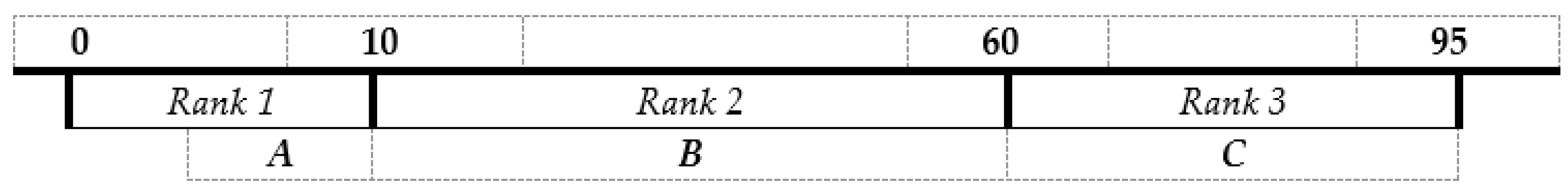
Figure 1), although for the other species (average in vulnerability values) there is uncertainty of such estimates shown above. On the other hand, a list of factors identifying birds’ vulnerability to oil was determined during such studies [14,33,34,35,36,37]. Specific metric values of a range of parameters, which are necessary for further researches and estimation of vulnerability were identified (Factors a, b, c and, d, see [36]).
Ordinal quantities in arithmetic operations should be abandoned when calculating the vulnerability of individual species or their groups. The development of appropriate models (calculation formulas) of vulnerability is required which would include only metric values on ratio scales. This can significantly complicate the models (formulas) used, since it would no longer be possible to simply sum or average several heterogeneous parameters of different nature and different units of measurement. Such an approach, based on the use of metric data in calculations, is proposed [30,31,32] for vulnerability assessments of different ecological groups of biota to oil and for development, on those bases, of vulnerability maps of sea-coastal zones to oil.
At the same time, one should also take into account the possibility of strictly correct expert assessment of parameters characterizing anthropogenic factors affecting seabirds, while receiving data on a ratio scale. This could include multicriteria decision analysis techniques such as the analytic hierarchy process (AHP). In fact, the method of pairwise comparison, as described in [38], allows making this. The obtained estimates can be considered to be quantities on a ratio scale. The correctness of the obtained values is controlled by the corresponding criteria [38]. For example, AHP was used to evaluate and integrate expert opinion on the risks posed to 14 species of seabird in NW Atlantic [39]. AHP is an effective tool to rank and prioritize conservation concerns, and it can help to guide conservation planning and management decisions. If used correctly, this method could overcome, to some extent, issues associated with calculations based on ordinal data.

Author Contributions

A.S. and A.K. reviewed the presented approaches and wrote the paper. All authors have read and agreed to the published version of the manuscript.

Funding

This research was funded by Ministry of Science and Higher Education of the Russian Federation.

Acknowledgments

This paper is based on the results of scientific research performed for the state assignment of MMBI RAS.

Conflicts of Interest

The authors declare no conflict of interest.

Appendix A. Definition of Concepts

Below are a number of key concepts and definitions (quantity, quantity-value scale, and measurement) from International Vocabulary of Metrology: Basic and General Concepts and Related Terms (VIM-3) [26].
Quantity (item 1.1) The property of a phenomenon, body, or substance, where the property has a magnitude that can be expressed as a number and a reference.
Quantity-value scale, measurement scale (item 1.27) The ordered set of quantity values of quantities of a given kind of quantity used in ranking, according to magnitude, quantities of that kind, for example, (1) Celsius temperature scale, (2) time scale, and (3) Rockwell C hardness scale.
Measurement (item 2.1) The process of experimentally obtaining one or more quantity values that can reasonably be attributed to a quantity. Note the following: (1) Measurement does not apply to nominal properties. (2) Measurement implies comparison of quantities or counting of entities. (3) Measurement presupposes a description of the quantity commensurate with the intended use of a measurement result, a measurement procedure, and a calibrated measuring system operating according to the specified measurement procedure, including the measurement conditions.

Appendix B. Additional Information on Some Scales

Appendix B.1. Scales of Denominations

These reflect actual qualitative properties. In such a scale (another name for it is nominal and sometimes the classification scale), all mutually unambiguous transformations are permissible and numbers are used only as labels. This scale, for instance, “measures” phone numbers or car plates. “Measurement” of this scale is used only to distinguish between objects [23]. Permissible transformations are carried out from time to time in real life, for example, when replacing phone numbers. Moreover, each previous telephone number corresponds to one and only one new one. It is not allowed that the two previous numbers merge, or that two new ones come out of the same one; this means that the transformation is mutually unambiguous [23]. In the International Vocabulary of Metrology (VIM-3) [26] there is no concept of a nominal scale, since, if a strict approach is taken, it is practically meaningless to talk about measurement on this scale.

Appendix B.2. Ordinal Scales

These allow monotonic transformations, and zero may be present or absent on these scales [27]. Numbers are used to distinguish between objects and also to establish order between them. In this scale, all strictly (monotonously) increasing transformations are permissible. Therefore, if an object xi is preferable to an object xj, any permissible transformation φ is such that φ(xi) > φ(xj) for all the objects xi and xj. In various areas of human activity, many types of ordinal scales are used, for example, the Mohs scale is used in mineralogy (a mineral with a higher number is harder than a mineral with a lower number). The ordinal scales in geography are the Beaufort wind force scale (calm, weak wind, moderate wind, etc.), or the Richter magnitude scale. Once again, citing the indicated document of the International Bureau of Weights and Measures (item 1.26), “no algebraic operations among ordinal quantities exist, and differences and ratios of ordinal quantities have no physical meaning” [26].

Appendix B.3. Interval and Difference Scales

In the interval scale, the value of potential energy, the coordinate of a point on a straight line, geographical latitude, and temperature in Celsius, Fahrenheit, or Réaumur scales are measured. The natural origin and the natural unit of measurement cannot be defined here. They are chosen by specialists, but the arbitrariness of such choice is obvious (for example, in the case of geographical latitude). Permissible transformations in the interval scale are linear incremental transformations, that is, linear functions. Therefore, the temperature scales of Celsius and Fahrenheit are connected by such dependence:
= 5 9 ( 32 ) ,
where °C is the temperature in the Celsius scale, and °F is the temperature in the Fahrenheit scale. In the interval scale, the ratio of the interval lengths for any numbers x 1 , x 2 , x 3 , x 4 (measurement results) and any permissible transformation φ(x) = ax + b, a > 0 is saved:
x 1 x 2 x 3 x 4 = φ ( x 1 ) φ ( x 2 ) φ ( x 3 ) φ ( x 4 ) ,
Let there be four temperature values on the Fahrenheit scale as follows: 212 °F, 167 °F, 122 °F, and 32 °F. The corresponding temperature values on the Celsius scale are as follows: 100 °C, 75 °C, 50 °C, and 0 °C. The ratio of the intervals of temperatures for them are as follows: on the Fahrenheit scale (122 − 32)/(212 − 167) = 2 and it is preserved on the Celsius scale (50 − 0)/(100 − 75) = 2.
However, not all the arithmetic operations are possible even with numerical values obtained using metric units. If the intervals on the scale are constant, as in ordinary measurements of temperature in Celsius, then, certain comparisons on this interval scale can be meaningless. It is incorrect to say that a body with the temperature of 100 °C is twice as warm as with the temperature of 50 °C (for Fahrenheit scale 212 °F/122 °F = 1.74). Only an interval scale with an absolute zero allows meaningful comparisons. Setting a natural zero for such scales is possible, for instance, on the absolute temperature scale (Kelvin scale) or length scales, that is, on such a metric scale, i.e., the interval scale, not all arithmetic operations are permissible.
There is a natural unit of measure in the difference scale, but there is no natural origin. Permissible transformations here are shifts. Time is measured on a scale of differences if the year (or day from noon to noon) is taken as the natural unit of measurement, and on a scale of intervals, it is measured in the general case. At the current level of knowledge, the natural time origin cannot be indicated. With permissible transformations, the difference in the measured values is preserved in the difference scale as,
x 1 x 2   =   φ ( x 1 ) φ ( x 2 ) ,
for any numbers x 1 and x 2 (results of measurements) and any admissible transformation φ(x) = x + b.
Scales of differences (intervals) differ from ordinal scales, for the properties they describe, i.e., the equivalence and ordinal relationships make sense and also the equality and summation of the intervals (differences) between different quantitative manifestations of the properties. A typical example is the scale of time intervals. Time intervals (for example, work or study periods) can be added and subtracted, but it is pointless to add the dates of any events. Another example is the scale of lengths (distances), i.e., spatial intervals, which is determined by combining the ruler zero with one point, and the counting is done at another point. Scales of this type include practical temperature scales with a conditional zero. Difference scales have conditional (accepted by agreement) units of measure and conditional zeros based on any benchmarks. In these scales, linear transformations are permissible; the procedures for finding the mathematical expectation, standard deviation, etc. are applicable in them [27].

Appendix B.4. Ratio Scales

This is the most used quantitative scale in science. It has a natural origin, i.e., zero, that is, the absence of a quantity, but there is no natural unit of measurement. Equivalence and ordinal relations, subtraction and multiplication operations (ratio scales of the first type, i.e., proportional scales), and in many cases summation (ratio scales of the second type, i.e., additive scales) are applicable to the set of quantitative manifestations in these scales [27]. There are conditional (accepted by agreement) units and natural zeros; these are widely used in physics and technology; all the arithmetic operations are allowed in them, except for summation in scales of the first type [27]. Permissible transformations are similar transformations (changing only the proportion), in other words, linear incremental transformations without a constant term [23]. With permissible transformations, the ratio of measured quantities is preserved in the ratio scale,
x 1 x 2 = φ ( x 1 ) φ ( x 2 ) ,
for any numbers x 1 and x 2 (results of measurements) and any permissible transformation φ(x) = ax, a > 0.
In the ratio scale, values of one scale can be converted to another scale of values by multiplication by a positive constant (for example, kilometers into nautical miles by multiplying by a factor of 1.852, or y = ax). Moreover, the ratio of two ordered observations (on the ratio scale) when they are multiplied by a constant is preserved; however, in the interval scale it changes with a permissible transformation (on the Celsius scale, one ratio, on the Fahrenheit scale, another, although these are the same temperature states of the substance, see the example in Section 2.3 above).
Given the importance of the ratio scale for further study, we present useful considerations on these scales from [38]. One can add up a couple of elements of the same scale and get a third element that belongs to the same relationship scale. Therefore, if y = ax and y’ = ax’, then y + y’ = a(x + x’), and the factor remains equal to a. However, neither the product nor the quotient of two such elements belongs to the same ratio scale. Therefore, if yy’ = a2xx’ and y y/y’ = x/x’, neither of these two elements belongs to the original ratio scale y = ax, since the factor a is absent in both.
Notably, the sum of two elements from two different ratio scales does not belong to any ratio scale. Nevertheless, the product and the quotient belong to a ratio scale that differs from the original ratio scales if a or b are not equal to 1. This can be verifies as follows: y = ax and y’ = bx makes y + y’ = ax +bx, yy’ = (ab)xx’ and y/y’ = (a/b)x/x’. Thus, working with two different ratio scales and wanting to get significant numbers in the new ratio scale, one should multiply and divide, but not add or subtract. That is why adding such quantities as time and distance makes no sense, but one can extract the meaning from dividing the distance by time, obtaining the speed [38].

Appendix B.5. Absolute Scales

Only for the absolute scale, the results of measurements are numbers in the usual sense of the word. An example, here, is the number of people in a room or the number of birds in a colony. For an absolute scale, only the identity transformation is permissible. Table A1 shows the characteristics of the six main types of measurement scales.
Table A1. Characteristics and features of scales of various types [23,27,45,46].
Characteristic of Measurement Scale Type Measurement Scale type
NominalOrdinalIntervalsDifferencesRatioAbsolute
Permissible logical relations between manifestations of propertiesEquivalence, difference in propertiesEquivalence, difference, orderEquivalence, order, proportionality, or summation of intervalsEquivalence, order, proportionality (for some, summation)Equivalence, order, proportionality, sometimes summation
Presence of zero (origin)SenselessNot necessaryBy agreementIntroduced naturally
Presence of measurement unitSenselessBy agreementDimensionless quantity
Need for a scale standardCan be implemented without a special standardImplemented by means of special standards or standards of other scalesNo need
Permissible transformationsAll mutually unambiguous transformations
x → x’ = φ(x)
where φ(x) is the mutually unambiguous correspondence law
All strictly monotonic transformations
x → x’ = φ(x)
where φ(x) is the monotonic function
All linear transformations
x → x’ = φ(x) = ax + b,
where a and b
are arbitrary,
a > 0
All shift transformations
x → x’ = φ(x) = x + b,
where b is arbitrary
All similar
Transformations
x → x’ = φ(x) = ax,
where a is arbitrary, a > 0
Only identical transformations
x → x’ = φ(x) = x
Applicability of arithmetic meanNot applicableApplicable
Applicability of medianSometimes applicableApplicableSometimes applicable
ExamplesPhone numbers, Odor Awareness ScaleExpert assessments, wind scores, school grades, house numbersPotential energy, Celsius and Fahrenheit temperatureWorld time scale, calendarsThermodynamic temperature scale, mass, length, power, currency conversionNumber of birds, particles, amount of information
Allowable transformations are those transformations that do not change the relationship between the measurement objects and, accordingly, the conclusions drawn from the measurement results.

Appendix B.6. Expert Assessments and Ratio Scales Based on Expert Assessments

Saaty’s [38] hierarchy analysis method is based on pairwise comparisons where experts do not rank the estimated parameters on a scale of “more–less” but conduct comparative assessments of the ratios of pairs of quantities.
This method can be described as follows: The analysis is based on the hierarchy method. Supposing elements of one level, for instance, the fourth level of the hierarchy and one element of the next higher level are specified. It is necessary to compare the elements of the fourth level in pairs by the strength of their influence on the selected element of the higher level, put the numbers reflecting the agreement reached in the comparison in the matrix, and find the eigenvector of this matrix with the largest eigenvalue. The eigenvector provides an ordering of priorities, and the eigenvalue is a measure of consistency of judgments [38].
Saaty [38] writes that L. Vargas in his thesis showed that the method of analyzing hierarchies was a measurement method. Firstly, he formulated a set of axioms that characterized the existence of a homomorphism between the set of alternatives and the set of positive real numbers (representation theorem). Second, he showed that homomorphism was unique up to a similarity transformation (uniqueness theorem), i.e., the set of permissible homomorphism transformations was a set of similarity transformations. Thus, the triple consisting of set alternatives, set of positive real numbers (or its uncountable subset), and homomorphism, was a ratio scale, however, only in its narrow sense, i.e., its elements do not change during the transformation. He also emphasized that the hierarchical dimension included the main and derived dimensions, and that the result was a ratio scale unique up to the same similarity transformation as the second level of the hierarchy (for more details see [38]).

Appendix B.7. Arithmetization of Ordinal Quantities

Often, a sequence of expertly assessed ordinal quantities is simply set without zero as an origin reference point, without a unit of measurement, and without indicating the boundaries of the intervals for ordinal quantities. This is how many calculations are often performed, including the sensitivity/vulnerability assessment for seabirds from anthropogenic influences (the analysis is given in the main text), and how maps of the vulnerability of coastal-marine zones from oil are constructed, which is described in [30]. In this case, arithmetic operations lead to errors. In fact, such use of ordinal quantities means a methodologically incorrect foundation of calculations. To use such ordinal quantities in addition and multiplication operations, their preliminary arithmetization is necessary [24,25]. When arithmetizing a linear ordinary scale, all measurement results on this scale that are not numerical take the form of numerical information. The development of various methods of arithmetization, also called “digitization” and “attribution of numerical marks”, can be widely used for processing non-numeric (ordinary) measurements most developed methods of modern mathematical statistics that is initially focused only on numerical source information [25].
The insufficiency of the linear scale structure makes it impossible to calculate the simplest statistical characteristics (average, variances, regression coefficients, etc.) even for ordinary information. Therefore, it is advisable to use additional information about possible gradations of quality, measured on a linear ordinal scale, to compare points [25] of this scale with some real numbers, and therefore one can speak about measuring this quality on a scale where addition and multiplication operations are permissible. The success of the application of the arithmetic procedure is facilitated by the fact that for many ordinary scales there is often additional information that allows possibly choosing a single function f(x) which arithmetizes a linear ordinary scale, or at least, determining a narrow class of permissible arithmetizations [25].

Appendix B.8. Summary Notes on Arithmetic Operations with Values on Different Scales

Thus, it can be assumed that arithmetic operations with quantities are permissible only on the scale of differences (multiplication is excluded), ratio, and the absolute scales (addition, multiplication). Since in the environmental studies under consideration (on the effects of anthropogenic factors on seabirds), the scale of differences is practically not used, only two scales remain for such operations, i.e., ratio and absolute. On the ordinal scale, such arithmetic operations are not allowed. Otherwise, if the results are presented using arithmetic operations (both addition and multiplication), then, the researcher assumes or accepts that it is either an absolute scale or a ratio scale, which means that a zero of scale and unit of measurement are defined, and various arithmetic operations are possible with the data, but this is not an ordinal scale. The use of ordinal quantities in arithmetic calculations is possible only after their preliminary arithmetization.

Appendix C. Examples of Arithmetic Operations with Ordinal Quantities: Summation and Multiplication

Below are examples of arithmetic operations with ranks (ordinal quantities) without arithmetization. In these examples, the ranks (scores) characterize some values relative to each other, experts who conduct these assessments do not know these values themselves or the interval boundaries for them on the real metric ratio scale. Let us consider the operation of summation (in fact, multiplication as multiple addition), and demonstrate with examples its unacceptability on an ordinal scale as follows:
Example A1.
Let it be required to evaluate some quantities A, B, and C, and then, carry out arithmetic operations with them. Supposing they were estimated by experts, and it was found that A is minimal as compared with B and C, therefore, it is assigned Rank 1, R(A) = R(1) = 1 (Figure A1). B has the average (intermediate) value, it is assigned Rank 2, R(B) = R(2) = 2. The maximum value is C and it is assigned Rank 3, R(C) = R(3) = 3. Then, the ”addition” of three ranks of A or three ranks similar in real values to A should give Rank 3 for this sum corresponding to C, 1 + 1 + 1 = 3. That is, using rank numbers as digits (and not as marks, ordinal numbers) and performing arithmetic operations with them, one gets the rank of the real value of C. Thus, it is assumed that R(1) × 3 = R(3) or, which is the same R(1) + R(1) + R(1) = R(3), which corresponds to the value of C. But for the values of A, B and C, the intervals on a real metric scale are not known to experts or to anyone else. It is only known that on the metric scale, the value of A is less than that of B, and all of them are less than the values of C. Therefore, in reality, the following situation can be observed, as shown in Figure A1.
Figure A1. Illustration of Example A1. Above are the metric scale parameters unknown to experts, below are the ranks corresponding to the values of the estimated quantities. The second interval on the metric (relative) scale for the quantity B is much larger than the first interval corresponding to the quantity A. However, all this ratio of the boundaries of the intervals is unknown to experts when evaluating quantities A, B, and C using the ranks as numbers.
Jmse 08 01026 g0a1
Example A2.
Naturally, it can be vice versa if the numerical values of the boundaries of the first interval are relatively far from the beginning (from zero) of the scale, and the intervals corresponding to all Ranks R(1), R(2), R(3), and R(4) are small and approximately equal (Figure A2). Then, one can get the following (as a result of actions with ordinal quantities A, B, C, D). The sum of two Ranks R(1) + R(1) (using rank marks as numbers) as corresponding to the real values should give Rank R(2), 1 + 1 = 2, which corresponds to the real value of B. Yet in reality, the true values of the sum of two values of A will correspond to a real value with a rank even greater than Rank 4, corresponding to the value of D, and not Rank 2 for the value of B (Figure A2). The sum of R(1) + R(1) can be larger than R(4), since even 100 + 100 > 150. In this case, it can be argued that in fact R(1) × 2 > R(4), or 1 × 2 > 4 (more likely, “1” × 2 > “4”).
That is, replacing the real values of the quantities with the numbers in which the ranks are expressed, and using these numbers as the “values” of the quantities, one gets that the “sum” of the two Ranks R(1) does not correspond to Rank R(2) but will correspond to the value with a rank even greater than with Rank R(4). All such actions ultimately lead to incorrect results and conclusions.
Figure A2. Illustration of Example A2. All intervals corresponding to the ranks are approximately equal, but this ratio of intervals and the origin of the scale is unknown to experts in assessing the values of the corresponding quantities.
Jmse 08 01026 g0a2
Here, it is necessary to turn once again to the properties of ordinal scales (Section Appendix B.2 of Appendix B). For an ordinal scale, it is impossible to establish the equality of intervals on different parts of the scale; for such quantities there are no algebraic operations between them.

References

  1. International Maritime Organization (IMO); International Petroleum Industry Environmental Conservation Association (IPIECA). Sensitivity Mapping for Oil Spill Response; IPIECA: London, UK, 1994; Volume 1. [Google Scholar]
  2. NOAA. Environmental Sensitivity Index Guidelines; NOAA Technical Memorandum NOS OR&R 11, Ver. 3.0; NOAA: Seattle, WA, USA, 2002; Available online: https://www.researchgate.net/publication/311924018_Environmental_Sensitivity_Index_Guidelines_Version_30 (accessed on 6 October 2020).
  3. International Petroleum Industry Environmental Conservation Association (IPIECA); International Maritime Organization (IMO); International Association of Oil & Gas Producers (OGP). Sensitivity Mapping for Oil Spill Response; IPIECA: London, UK, 2012; Available online: https://www.ipieca.org/resources/good-practice/sensitivity-mapping-for-oil-spill-response/#:~:text=Sensitivity%20maps%20convey%20essential%20information,spill%20response%20should%20be%20included (accessed on 6 October 2020).
  4. Shavykin, A.A. (Ed.) Kola Bay and Oil: Biota, Vulnerability Maps, Pollution; Renome: St. Petersburg, Russia, 2018. (In Russian) [Google Scholar] [CrossRef]
  5. Offringa, H.R.; Låhr, J. An Integrated Approach to Map Ecologically Vulnerabilities in Marine Waters in the Netherlands (V-Maps); RIKZ working document RIKZ 2007-xxx; Ministry of Transport, Public Works and Water Management, Rijkswaterstaat, National Institute for Marine and Coastal Management: Hague, The Netherlands, 2007; Available online: https://library.wur.nl/WebQuery/wurpubs/358188 (accessed on 6 October 2020).
  6. Admiral Danish Fleet, H.Q. Sub-Regional Risk of Spill of Oil and Hazardous Substances in the Baltic Sea (BRISK). Environmental Vulnerability; Doc. No. 3.1.3.3, Ver. 1; Admiral Danish Fleet HQ, National Operations, Maritime Environment: Copenhagen, Denmark, 2012. [Google Scholar]
  7. International Council for the Exploration of the Sea (ICES). Report of the Working Group on Seabird Ecology; Oceanography Committee, ICES CM 2002/C:04, Ref. ACME, ACE, E and F, ICES Headquarters, 8–11 March 2002; ICES: Copenhagen, Denmark, 2002; Available online: http://www.ices.dk/sites/pub/CM%20Doccuments/2002/C/C0402.PDF (accessed on 6 October 2020).
  8. Garthe, S.; Hüppop, O. Scaling possible adverse effects of marine wind farms on seabirds: Developing and applying a vulnerability index. J. Appl. Ecol. 2004, 41, 724–734. [Google Scholar] [CrossRef]
  9. Camphuysen, C.J. Chronic Oil Pollution in Europe; Report Royal Netherlands Institute for Sea Research; Commissioned by International Fund for Animal Welfare (IFAW): Brussels, Belgium, 2007; Available online: https://no0ilcanarias.files.wordpress.com/2013/05/chronic-oil-pollution-in-eu.pdf (accessed on 6 October 2020).
  10. Furness, R.W.; Wade, H.M.; Masden, E.A. Assessing vulnerability of marine bird populations to offshore wind farms. J. Environ. Manag. 2013, 119, 56–66. [Google Scholar] [CrossRef] [PubMed]
  11. Bradbury, G.; Trinder, M.; Furness, B.; Banks, A.N.; Caldow, R.W.G.; Hume, D. Mapping Seabird Sensitivity to Offshore Wind Farms. PLoS ONE 2014, 9, e106366. [Google Scholar] [CrossRef] [PubMed] [Green Version]
  12. Certain, G.; Jørgensen, L.L.; Christel, I.; Planque, B.; Bretagnolle, V. Mapping the vulnerability of animal community to pressure in marine systems: Disentangling pressure types and integrating their impact from the individual to the community level. ICES J. Mar. Sci. 2015, 72, 1470–1482. [Google Scholar] [CrossRef] [Green Version]
  13. O’Hanlon, N.J.; Bond, A.L.; James, N.A.; Masden, E.A. Oil Vulnerability Index, Impact on Arctic Bird Populations (Proposing a Method for Calculating an Oil Vulnerability Index for the Arctic Seabirds). In Arctic Marine Sustainability: Arctic Maritime Businesses and the Resilience of the Marine Environment; Pongrácz, E., Pavlov, V., Hänninen, N., Eds.; Springer: Cham, Switzerland, 2020; pp. 73–94. [Google Scholar] [CrossRef]
  14. Statens Forurensningstilsyn (SFT). Beredskap Mot. Akutt Forurensning—Modell for Prioritering av Miljøressurser ved Akutte Oljeutslipp Langs Kysten; TA-nummer 1765/2000; SFT: Oslo, Norway, 2004; Available online: https://www.miljodirektoratet.no/globalassets/publikasjoner/klif2/publikasjoner/vann/1765/ta1765.pdf (accessed on 6 October 2020). (In Norwegian)
  15. Pogrebov, V.B. Integral Assessment of the Environmental Sensitivity of the Biological Resources of the Coastal Zone to Anthropogenic Influences. In Basic Concepts of Modern Coastal Using; RSHU: St. Petersburg, Russia, 2010; Volume 2, pp. 43–85. Available online: https://www.researchgate.net/publication/275348635_Pogrebov_VB_Integralnaa_ocenka_ekologiceskoj_cuvstvitelnosti_bioresursov_beregovoj_zony_k_antropogennym_vozdejstviam_Osnovnye_koncepcii_sovremennogo_beregopolzovania_T_2_SPb_izd-vo_RGGMU_2010_S_43-85 (accessed on 6 October 2020). (In Russian)
  16. Shavykin, A.A.; Ilyn, G.V. An Assessment of the Integral Vulnerability of the Barents Sea from Oil Contamination; MMBI KSC RAS: Murmansk, Russia, 2010; Available online: http://www.mmbi.info/fs/files/424/AN__ASSESSMENT_OF_THE_INTEGRAL.pdf (accessed on 6 October 2020). (In Russian)
  17. World Wildlife Fund (WWF). Methodological Approaches to Ecologically Sensitive Areas and Areas of Priority Protection Map Development and Coastline of the Russian Federation to Oil Spills; World Wildlife Fund: Vladivostok, Russia; Moscow, Russia; Murmansk, Russia; St. Petersburg, Russia, 2012; Available online: http://rus-arc.ru/ShareFiles/Publications/Blinovskaya_et_al_wwf_oil_net.pdf (accessed on 6 October 2020). (In Russian)
  18. Shavykin, A.A. A method for constructing maps of vulnerability of coastal and marine areas from oil. Example maps for the Kola Bay. Bull. Kola Sci. Cent. RAS 2015, 2, 113–123. Available online: https://cyberleninka.ru/article/n/metodika-postroeniya-kart-uyazvimosti-pribrezhnyh-i-morskih-zon-ot-nefti-primer-kart-dlya-kolskogo-zaliva/viewer (accessed on 6 October 2020). (In Russian).
  19. Furness, R.W.; Wade, H.M.; Robbins, A.M.C.; Masden, E.A. Assessing the sensitivity of seabird populations to adverse effects from tidal stream turbines and wave energy devices. ICES J. Mar. Sci. 2012, 69, 1466–1479. [Google Scholar] [CrossRef] [Green Version]
  20. Stevens, S.S. On the Theory of Scales of Measurement. Science 1946, 103, 677–680. Available online: https://psychology.okstate.edu/faculty/jgrice/psyc3214/Stevens_FourScales_1946.pdf (accessed on 6 October 2020). [CrossRef] [PubMed]
  21. Stevens, S.S. Mathematics, measurement, and psychophysics. In Handbook of Experimental Psychology; Stevens, S.S., Ed.; Wiley: New York, NY, USA, 1951. [Google Scholar]
  22. Sachs, L. Statistische Auswertungsmethoden (Methods of Statistical Analysis), 3rd ed.; Springer: Berlin/Heidelberg, Germany, 1972. [Google Scholar] [CrossRef]
  23. Orlov, A.I. Organizational-Economic Modeling: In 3 Parts. Part. 2: Expert Evaluation; Bauman MSTU: Moscow, Russia, 2011; Available online: http://ebooks.bmstu.ru/catalog/153/book1069.html (accessed on 6 October 2020). (In Russian)
  24. Khovanov, N.V. The Mathematical Foundations of the Theory of Scales for Measuring Quality; Leningrad University: Leningrad, Russia, 1982. (In Russian) [Google Scholar]
  25. Khovanov, N.V. Analysis and Synthesis of Indicators in Information Deficit; SPbU: St. Petersburg, Russia, 1996; Available online: https://www.studmed.ru/hovanov-nv-analiz-i-sintez-pokazateley-pri-informacionnom-deficite_f0c8b2fce13.html (accessed on 6 October 2020). (In Russian)
  26. Joint Committee for Guides in Metrology (JCGM 200:2012). International Vocabulary of Metrology—Basic and General Concepts and Associated Terms (VIM), 3rd ed.; JCGM: Sèvres, France, 2012; Available online: https://www.bipm.org/utils/common/documents/jcgm/JCGM_200_2012.pdf (accessed on 6 October 2020).
  27. Recommendations for Interstate Standardization (RMG 83-2007). State System for Ensuring the Uniformity of Measurements. Scales of Measurements. Terms and Definitions, official ed.; Standartinform: Moscow, Russia, 2008; Available online: http://docs.cntd.ru/document/1200063408 (accessed on 6 October 2020). (In Russian)
  28. Shavykin, A.A.; Matishov, G.G.; Karnatov, A.N. A Procedure for mapping vulnerability of sea-coastal zones to oil. Dokl. Earth Sci. 2017, 475, 907–910. [Google Scholar] [CrossRef]
  29. Shavykin, A.A. The main problems of rank values use (Annex D). In Kola Bay and Oil: Biota, Vulnerability Maps, Pollution; Shavykin, A.A., Ed.; Renome: Saint Petersburg, Russia, 2018; pp. 463–472. (In Russian) [Google Scholar] [CrossRef]
  30. Shavykin, A.A.; Karnatov, A.N. Main Development Problems of Vulnerability Mapping of Sea-Coastal Zones to Oil Spills. J. Mar. Sci. Eng. 2018, 6, 115. [Google Scholar] [CrossRef] [Green Version]
  31. Shavykin, A.A.; Karnatov, A.N. Method for mapping sensitivity/vulnerability of sea-coastal zones to oil (Chapter 12). In Kola Bay and Oil: Biota, Vulnerability Maps, Pollution; Shavykin, A.A., Ed.; Renome: Saint Petersburg, Russia, 2018; pp. 292–317. (In Russian) [Google Scholar] [CrossRef]
  32. Shavykin, A.A.; Karnatov, A.N. Mapping of Ecological Vulnerability of Sea-Coastal Zones to Oil Spills: A Preliminary Method Applied to Kola Bay, the Barents Sea. J. Mar. Sci. Eng. 2019, 7, 216. [Google Scholar] [CrossRef] [Green Version]
  33. King, J.G.; Sanger, G.A. Oil vulnerability index for marine oriented birds. In Conservation of Marine Birds of Northern North America; Wildlife Research Report, 11, Bartonek, J.C., Nettleship, D.N., Eds.; United States Department of the Interior Fish and Wildlife Service: Washington, DC, USA, 1979; pp. 227–239. Available online: https://books.google.ru/books?hl=ru&lr=&id=AC8lAQAAMAAJ&oi=fnd&pg=PA227&ots=XILgnOCZ6W&sig=0gWhubt4Cymh2sEV9gg-lDoWKhM&redir_esc=y#v=onepage&q&f=false (accessed on 6 October 2020).
  34. Anker-Nilssen, T. Metoder til Konsekvensanalyser Olje/Sjøfugl, Viltrapport; NINA: Trondheim, Norway, 1987; Volume 44, pp. 1–114. Available online: https://www.nina.no/archive/nina/pppbasepdf/forskningsrapport/042.pdf (accessed on 6 October 2020).
  35. Speich, S.M.; Manuwal, D.A.; Wahl, T.R. “In my experience...” The bird/habitat oil index—A habitat vulnerability index based on avian utilization. Wildl. Soc. Bull. 1991, 19, 216–221. Available online: https://www.jstor.org/stable/3782334 (accessed on 6 October 2020).
  36. Williams, J.M.; Tasker, M.L.; Carter, I.C.; Webb, A. A method of assessing seabird vulnerability to surface pollutants. IBIS 1994, 137, S147–S152. [Google Scholar] [CrossRef]
  37. Gavrilo, M.; Bakken, V.; Firsova, L.; Kalyakin, V.; Morozov, V.; Pokrovskaya, I.; Isaksen, K. Oil Vulnerability Assessment for Marine Birds Occurring along the Northern Sea Route; INSROP Working Paper; ARCTIS Database: Kirkenes, Norway, 1998; Volume 97, Available online: http://www.arctis-search.com/Oil+Vulnerability+Assessment+for+Marine+Birds+occurring+along+the+Northern+Sea+Route (accessed on 6 October 2020).
  38. Saaty, T.L. The Analytic Hierarchy Process: Planning, Priority Setting, Resource Allocation; McGraw-Hill International Book Company: New York, NY, USA, 1980. [Google Scholar]
  39. Lieske, D.J.; McFarlane Tranquilla, L.; Ronconi, R.; Abbott, S. Synthesizing expert opinion to assess the at-sea risks to seabirds in the western North Atlantic. Biol. Conserv. 2019, 233, 41–50. [Google Scholar] [CrossRef]
  40. Suppes, P.; Zinnes, J.L. Basic measurement theory. In Handbook of Mathematical Psychology; Luce, R., Bush, R., Galanter, E., Eds.; John Wiley and Sons: New York, NY, USA; London, UK, 1963; Volume 1, pp. 1–76. [Google Scholar] [CrossRef]
  41. Velleman, P.F.; Wilkinson, L. Nominal, Ordinal, Interval, and Ratio Typologies Are Misleading. Am. Stat. 1993, 47, 65–72. [Google Scholar] [CrossRef]
  42. Pfanzagl, J. Theory of Measurement, (in cooperation with V. Baumann, H. Huber), 2nd ed.; Physica-Verlag: Wursburg, Germany; Vienna, Austria, 1971. [Google Scholar] [CrossRef]
  43. Orlov, A.I. Measurement theory as part of data analysis methods: Reflections on the translation of the article by P.F. Welleman and L. Wilkinson. Sociology 2012, 35, 155–174. Available online: https://www.jour.fnisc.ru/index.php/soc4m/article/view/3740/3501 (accessed on 6 October 2020). (In Russian).
  44. Knorring, V.G. Theoretical foundations of information-measuring technique. Basic concepts of scale theory. In Lecture Notes; Leningrad Polytechnic Institute named after M.I. Kalinin: Leningrad, Russia, 1983. (In Russian) [Google Scholar]
  45. Doynikov, A.S. Measurements scales. In Physical Encyclopedia; Scientific Publishing House “Great Russian Encyclopedia”: Moscow, Russia, 1998; Volume 5, pp. 465–466. (In Russian) [Google Scholar]
  46. Novikov, N.Y. Theory of Scales. Principles of Building Reference Measurement Procedures, Coding and Control, 2nd ed.; Fizmatgiz: Moscow, Russia, 2012; Available online: https://www.studentlibrary.ru/book/ISBN9785922111157.html (accessed on 6 October 2020). (In Russian)
  47. Zhukov, V.K. Metrology. Measurement Theory. Study Guide for Undergraduate and Graduate Studies; Urite: Moscow, Russia, 2016; Available online: https://urait.ru/bcode/434013 (accessed on 6 October 2020). (In Russian)
  48. Orlov, A.I. Sustainability in Socio-Economic Models; Nauka: Moscow, Russia, 1979. (In Russian) [Google Scholar]
  49. Manuwal, D.S.; Wahl, T.R.; Speich, S.M. The Seasonal Distribution and Abundance of Marine Bird Populations in the Strait of Juan de Fuca and Northern Puget Sound in 1978; U.S. Dep. Commer., Natl. Oceanic and Atmos. Adm., Tech. Memo. ERL, MESA-44; Environmental Research Laboratories: Boulder, CO, USA, 1979. [Google Scholar]
  50. Wahl, T.R.; Speich, S.M.; Manuwal, D.A.; Hirsch, K.V.; Miller, C. Marine Bird Populations of the Strait of Juan de Fuca, Strait of Georgia and Adjacent Waters in 1978 and 1979; Dep. of Comm., Environ. Prot. Agency Interagency Energy, Environ. Res. And Devel. Program Rep. 600/7-81-156, U.S. Environ. Prot. Agency; EPA: Washington, DC, USA, 1981. [Google Scholar]
  51. Mehlum, F.; Bakken, V. Seabirds in Svalbard (Norway): Status, recent, changes and management. Birdlife Conserv. Ser. 1994, 1, 155–171. [Google Scholar]
  52. Isaksen, K.; Bakken, V.; Wiig, Ø. Potential Effects on Seabirds and Marine Mammals of Petroleum Activity in the Northern Barents Sea; Meddelelser NR. 154; Norsk Polarinstitutt: Oslo, Norway, 1998; Available online: https://www.semanticscholar.org/paper/Potential-effects-on-seabirds-and-marine-mammals-of-Bakken-Wiig/ee4a8f1d634f48c80500230c5bcffbc50c32b95c (accessed on 6 October 2020).
  53. Zakarin, E.A.; Balakai, L.A.; Bostanbekov, K.A.; Dedova, T.V.; Kim, D.K.; Kobegenova, S.S.; Mirkarimova, B.M.; Nurseitov, D.B. Environmental Risks Modeling in Case of Oil Pollution in the Water Area of the North-East Caspian; IJASEIT: Almaty, Kazakhstan, 2016. [Google Scholar]
Figure 1. Dependence of the product of rank values of two series of data on the product of their metric values. The circled pairs of points show partially uncertain results of ordinal quantities multiplying as compared to metric values. The arrows indicate how these points, probably, have to be shifted from their position on the graph; but it is not clear which point in the pair should shift and how much.
Jmse 08 01026 g001
Table 1. An example of calculating the bird oil index (BOI) of two conditional types AAA and BBB at different values of the source data (differing by a monotonic transformation). The upper two lines correspond to the values of the components 0, 1, 3, 5, the lower two lines correspond to the values of 0, 1, 2, 3.
SpeciesX1X2X3X4X5Y1Y2Y3Y4Y5Z1Z2Z3Z4BOIRank
AAA5035510005330160.52
BBB1011115111315540.31
AAA3023310003220117.61
BBB1011113111213320.22
Table 2. The initial data of the values (a, b, c) and (f, g, h). Xm and Ym are the metric values of the initial data; Xr and Yr are the corresponding ranks.
XmXr YmYr
a51 f31
b102 g202
c503 h403
Table 3. Results of the multiplication of both metric and rank values of the source data.
Xm × YmXr × Yr
af151
bf302
ag1002
cf1503
ah2003
bg2004
bh4006
cg10006
ch20009
Publisher’s Note: MDPI stays neutral with regard to jurisdictional claims in published maps and institutional affiliations.

