Revisiting Vertical Land Motion and Sea Level Trends in the Northeastern Adriatic Sea Using Satellite Altimetry and Tide Gauge Data


Abstract
1. Introduction
2. Data
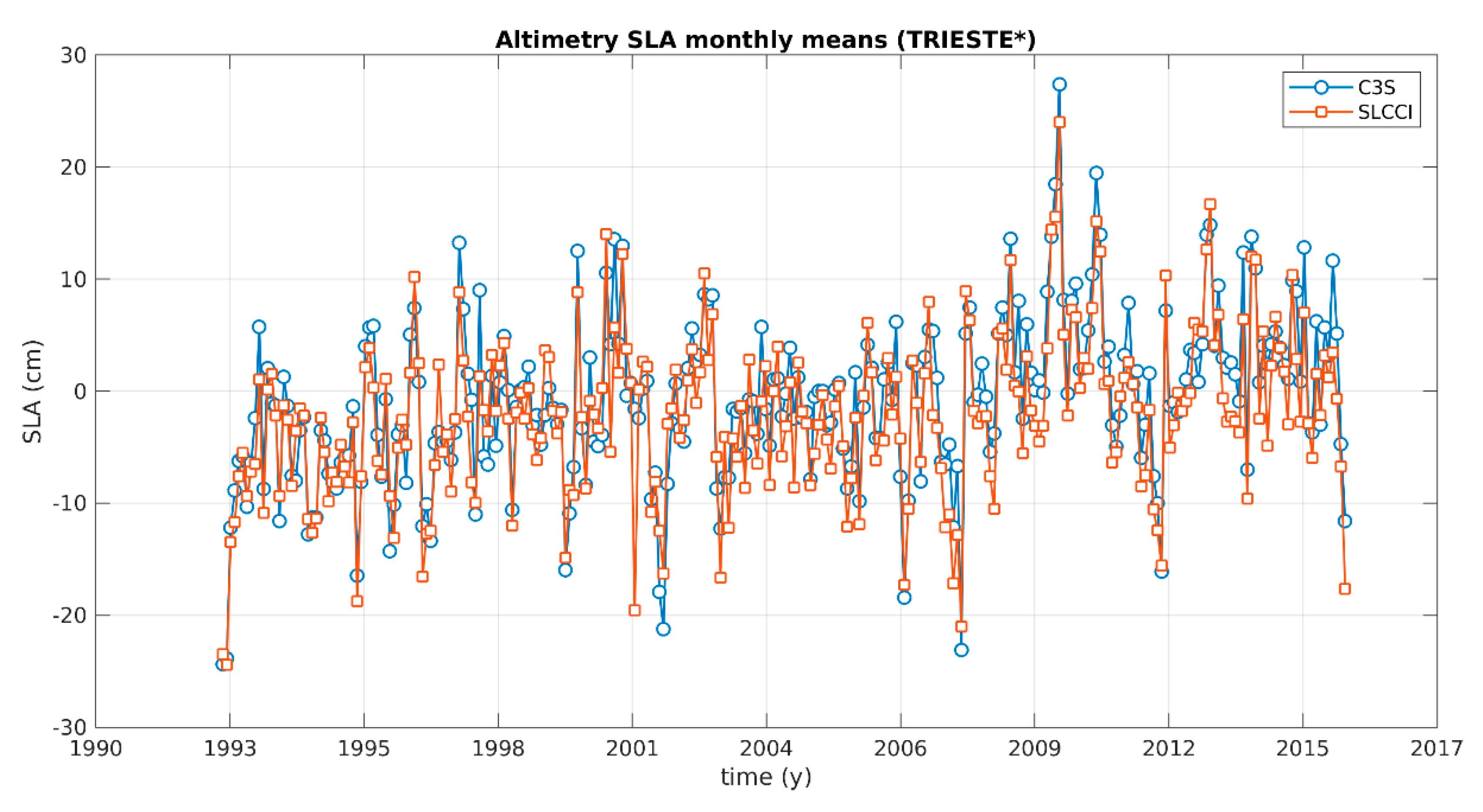
2.1. Altimetry Sea Level Datasets
2.1.1. SLCCI Altimetry SLA
2.1.2. C3S Altimetry SLA
2.1.3. Dynamic Atmospheric Correction and TOPEX-A Drift
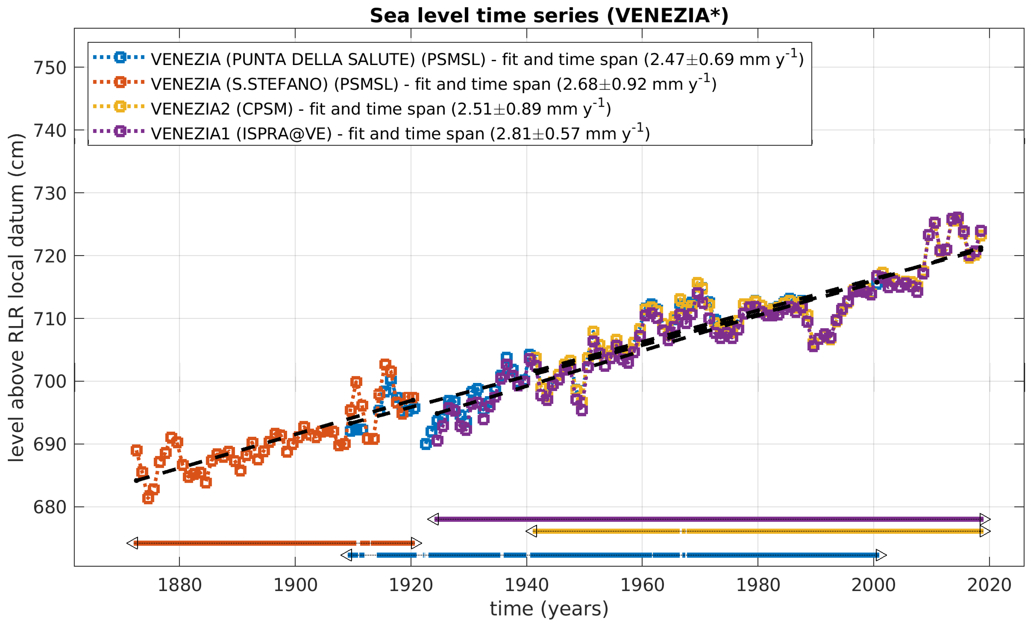
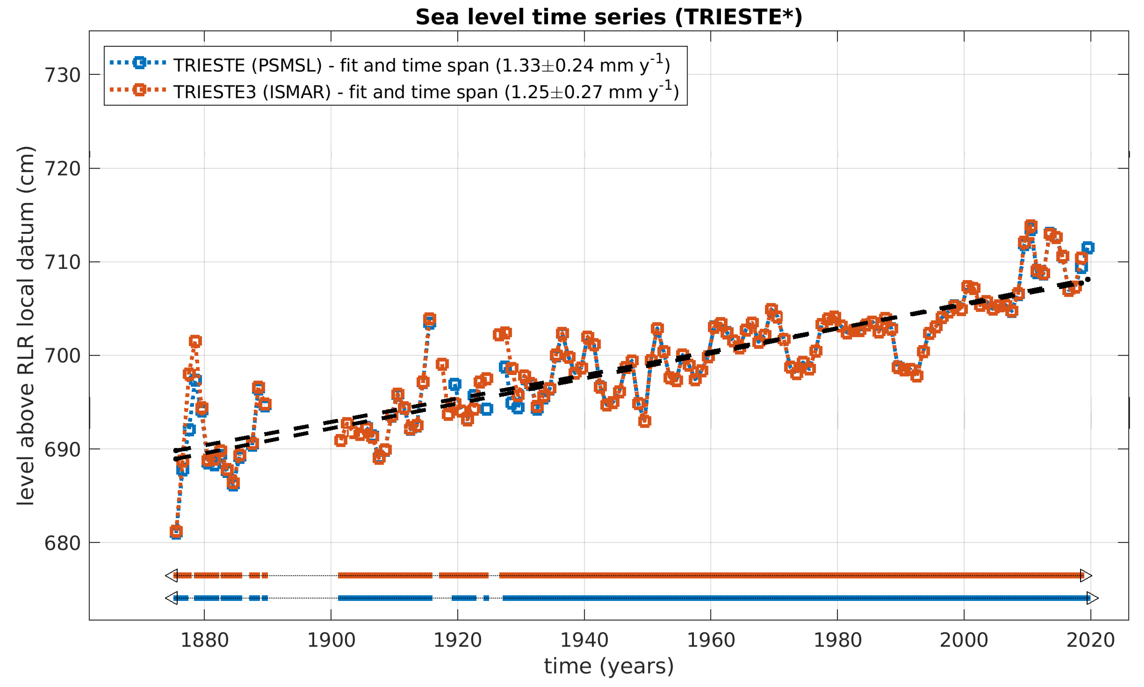
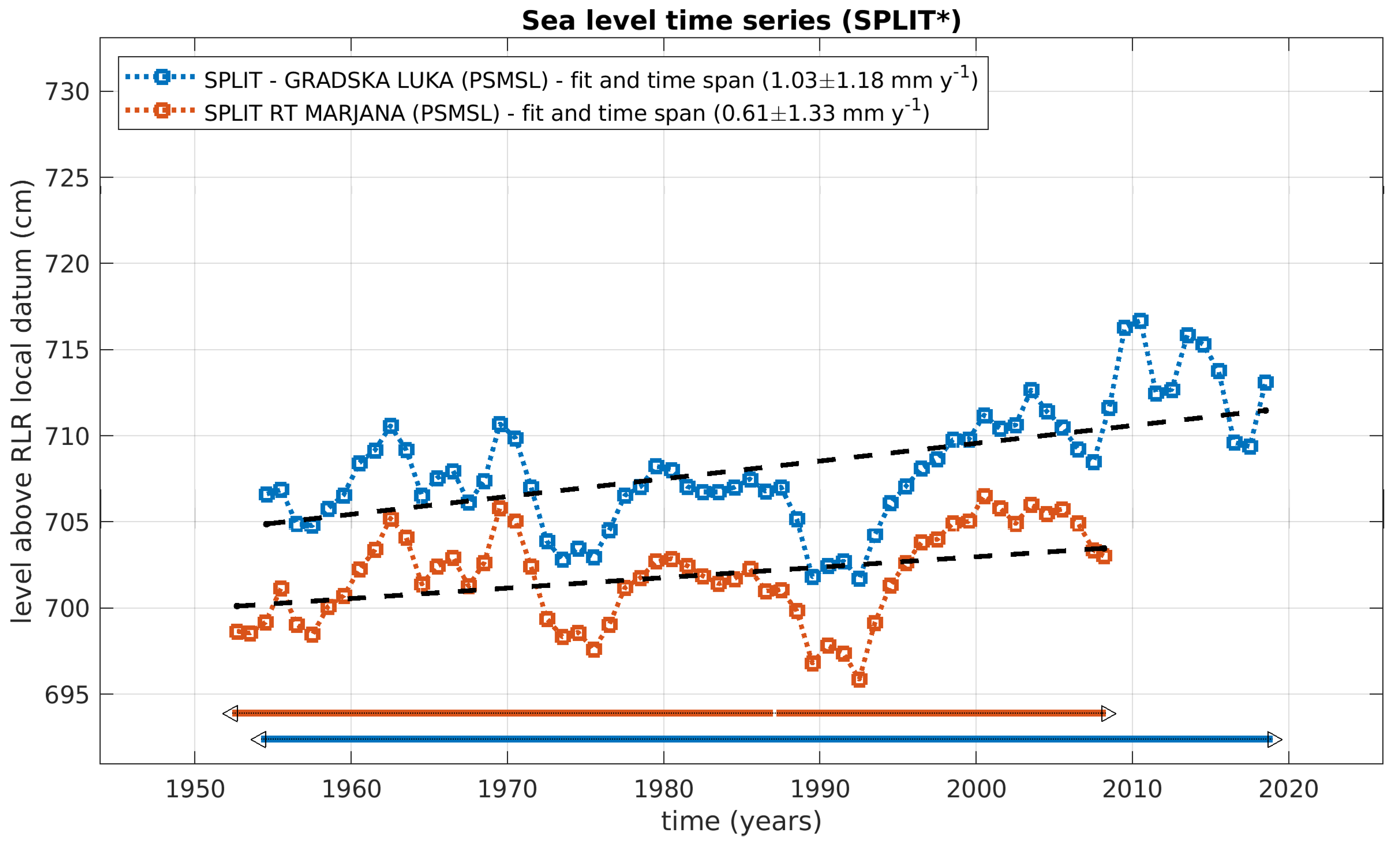
2.2. Tide Gauge Sea Level Dataset
2.3. Geocentric Surface Vertical Velocities from CGPS
3. Synergistic Use of Tide Gauge and Satellite Altimetry Data to Estimate Vertical Displacement Rates
3.1. Linear Inverse Problem with Constraints
3.2. A Possible Solution to the Limitation of the LIP Method
- (1)
- All the time series have a linear trend in every period in which they are considered;
- (2)
- The absolute sea level rates observed by satellite altimetry in its era can be extended backward in time to cover the timespan of the associated TG relative sea level time series.
4. Results
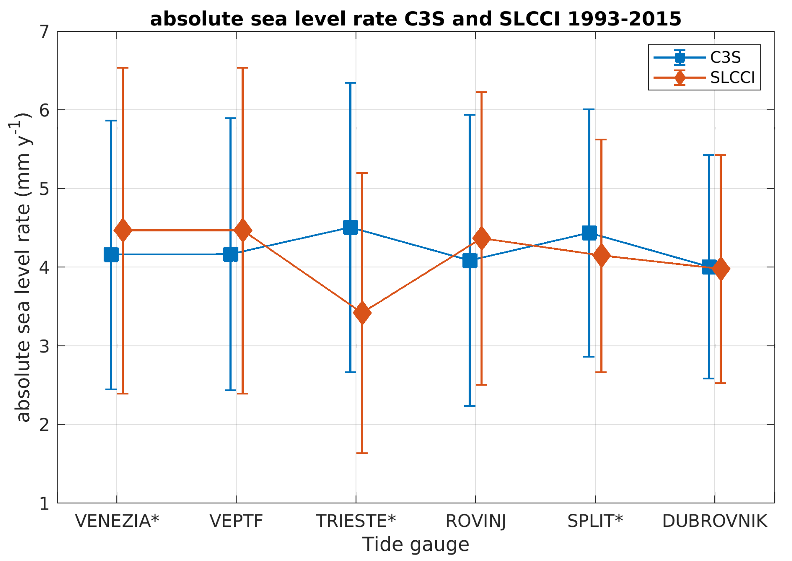
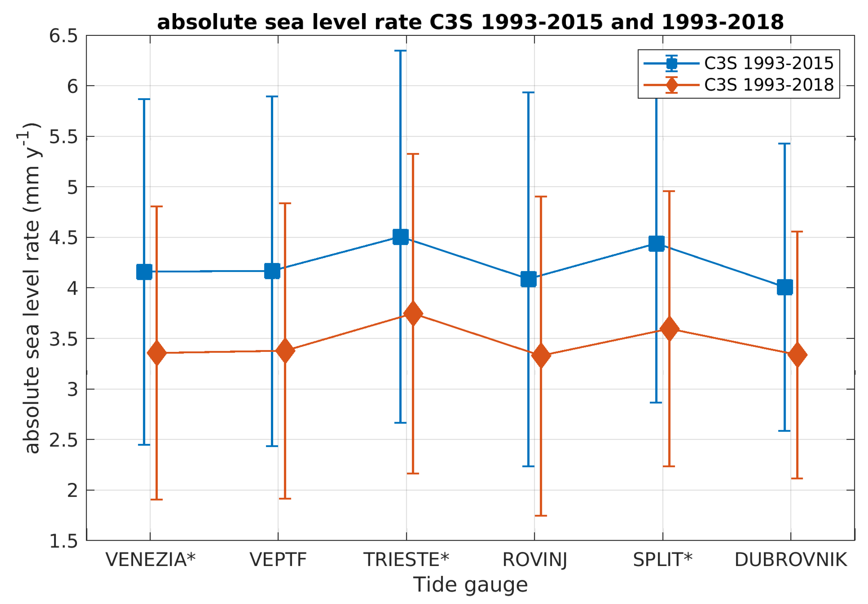
4.1. C3S and SLCCI Absolute Sea Level Change Rates 1993–2015
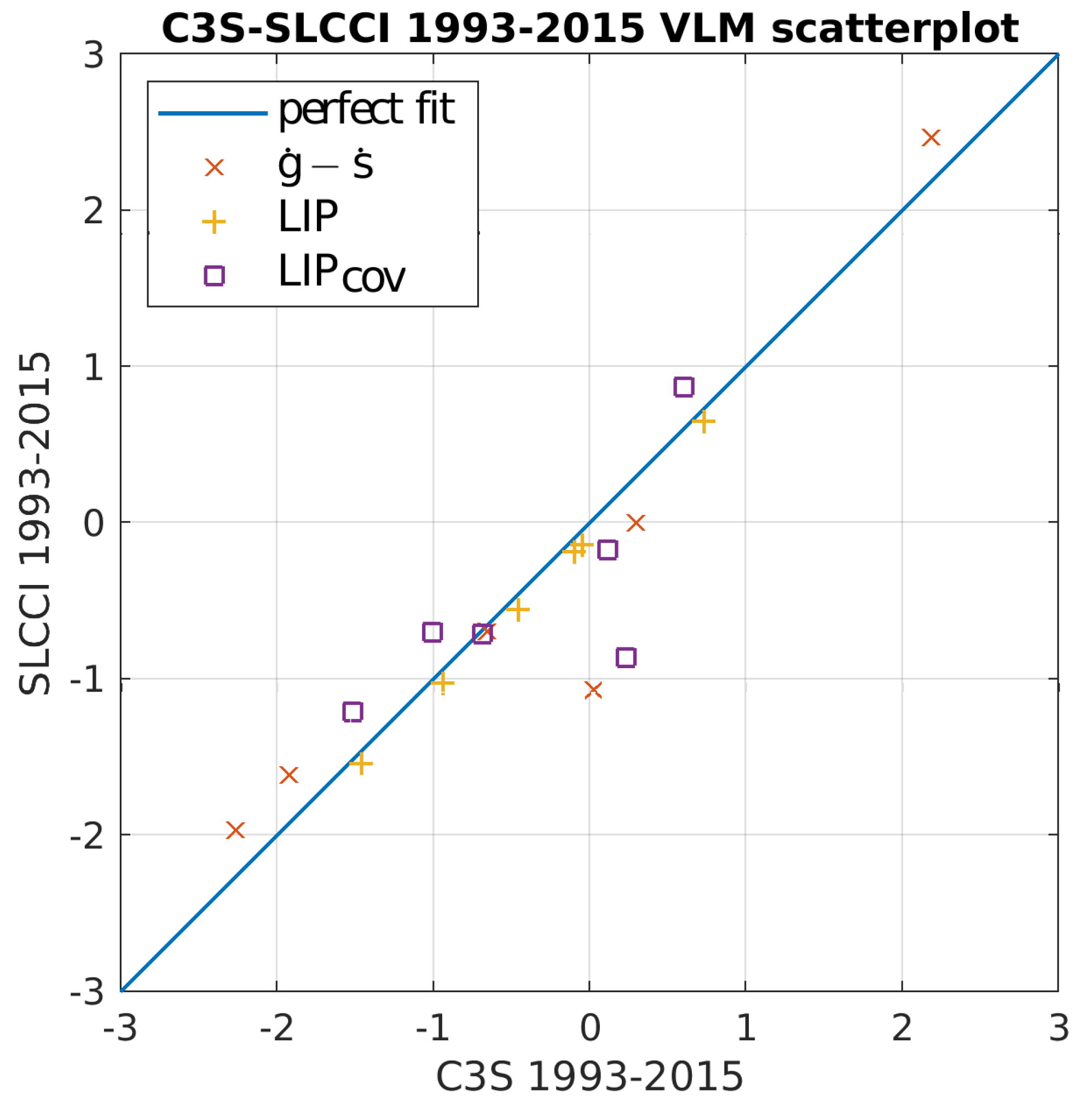
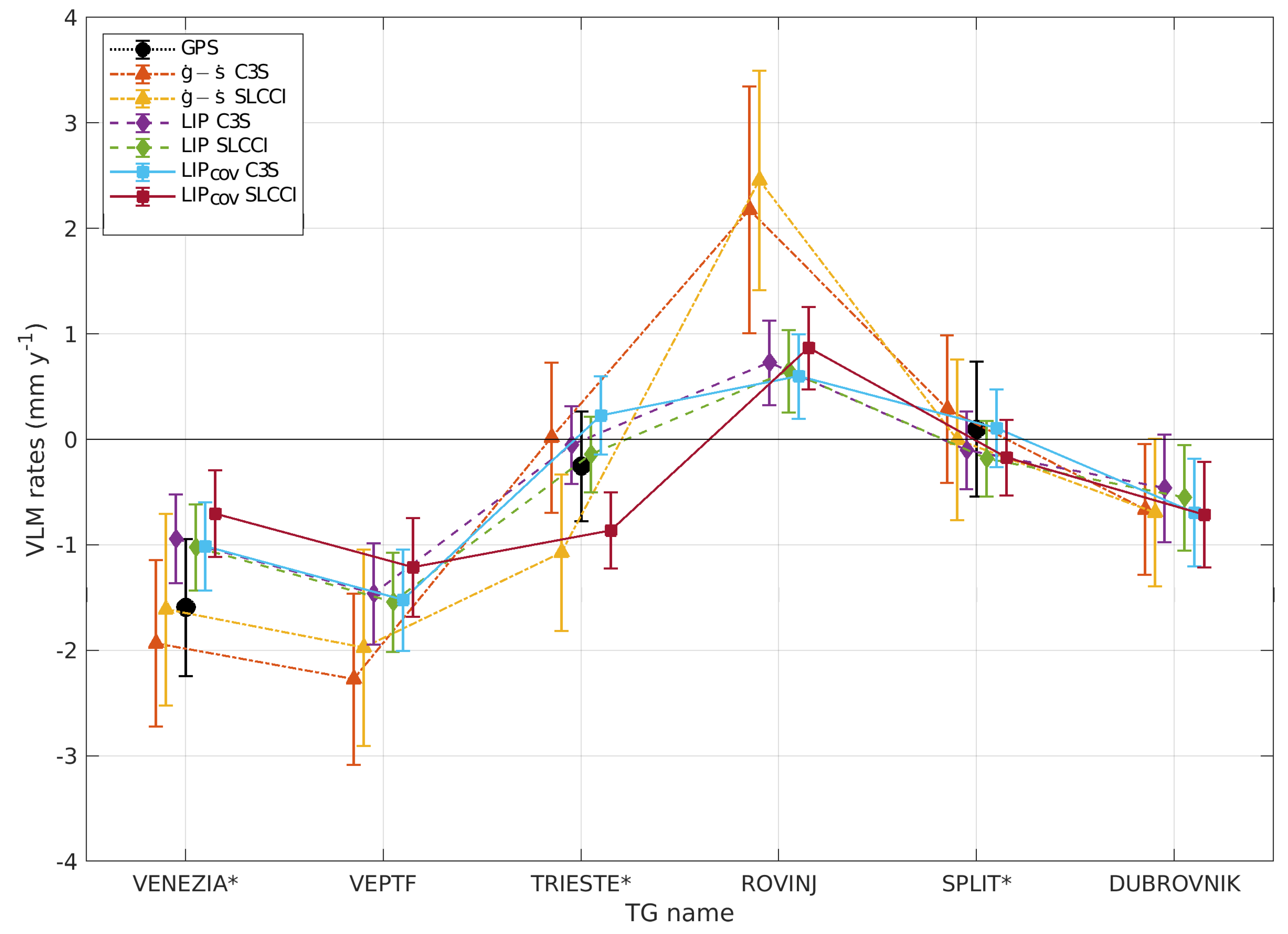
4.2. Vertical Land Motion Rates Derived with Standard (ALT-TG) and LIP Approaches 1993–2015
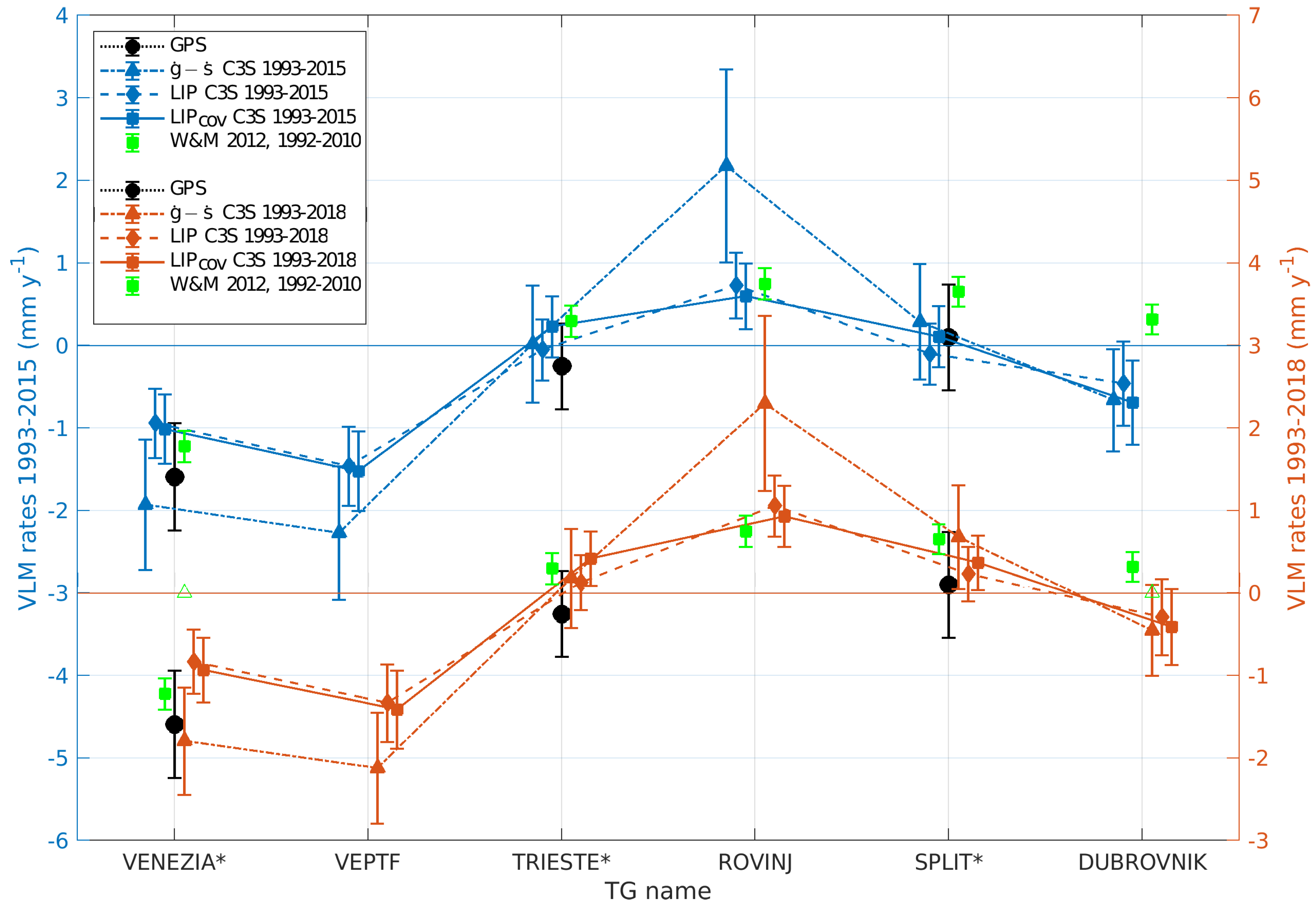
4.3. C3S Rates 1993–2018
- 1.36 ± 0.13 mm y−1 (19??–2010), W&M [9] (question marks indicate that the lower end of the period is different for each TG and coincident with the beginning of the observation period);
- 2.27 ± 0.41 mm y−1 (1974–2015), SLCCI, this study (not shown);
- 2.35 ± 0.20 mm y−1 (1974–2015), C3S, this study (not shown);
- 2.43 ± 0.18 mm y−1 (1974–2018), C3S, this study.
5. Discussion and Conclusions
Author Contributions
Funding
Acknowledgments
Conflicts of Interest
References
- Meyssignac, B.; Cazenave, A. Sea level: A review of present-day and recent-past changes and variability. J. Geodyn. 2012, 58, 96–109. [Google Scholar] [CrossRef]
- Chafik, L.; Nilsen, J.E.Ø.; Dangendorf, S.; Reverdin, G.; Frederikse, T. North Atlantic Ocean Circulation and Decadal Sea Level Change During the Altimetry Era. Sci. Rep. 2019, 9, 1041. [Google Scholar] [CrossRef] [PubMed]
- Međugorac, I.; Pasarić, M.; Güttler, I. Will the wind associated with the Adriatic storm surges change in future climate? Theor. Appl. Climatol. 2020. [Google Scholar] [CrossRef]
- Satellite Altimetry and Earth Sciences—A Handbook of Techniques and Applications, 1st ed.; International Geophysics; Fu, L.-L., Cazenave, A., Eds.; Academic Press, Inc.: San Diego, CA, USA, 2001; Volume 69, ISBN 978-0-12-269545-2. [Google Scholar]
- Gommenginger, C.; Thibaut, P.; Fenoglio-Marc, L.; Quartly, G.; Deng, X.; Gomez-Enri, J.; Challenor, P.; Gao, Y. Retracking altimeter waveforms near the coasts. In Coastal Altimetry; Vignudelli, S., Kostianoy, A.G., Cipollini, P., Benveniste, J., Eds.; Springer: Berlin/Heidelberg, Germany, 2011; pp. 61–102. [Google Scholar]
- Cazenave, A.; Dominh, K.; Ponchaut, F.; Soudarin, L.; Cretaux, J.F.; Le Provost, C. Sea level changes from Topex-Poseidon altimetry and tide gauges, and vertical crustal motions from DORIS. Geophys. Res. Lett. 1999, 26, 2077–2080. [Google Scholar] [CrossRef]
- Kuo, C.Y.; Shum, C.K.; Braun, A.; Mitrovica, J.X. Vertical crustal motion determined by satellite altimetry and tide gauge data in Fennoscandia. Geophys. Res. Lett. 2004, 31. [Google Scholar] [CrossRef]
- Kuo, C.Y.; Shum, C.K.; Braun, A.; Cheng, K.-C.; Yi, Y. Vertical Motion Determined Using Satellite Altimetry and Tide Gauges. Terrestrial. Atmos. Ocean. Sci. 2008, 19. [Google Scholar] [CrossRef]
- Wöppelmann, G.; Marcos, M. Coastal sea level rise in southern Europe and the nonclimate contribution of vertical land motion. J. Geophys. Res. Ocean. 2012, 117. [Google Scholar] [CrossRef]
- Zerbini, S.; Raicich, F.; Prati, C.M.; Bruni, S.; Conte, S.D.; Errico, M.; Santi, E. Sea-level change in the Northern Mediterranean Sea from long-period tide gauge time series. Earth-Sci. Rev. 2017, 167, 72–87. [Google Scholar] [CrossRef]
- Fenoglio-Marc, L. Long-term sea level change in the Mediterranean Sea from multi-satellite altimetry and tide gauges. Phys. Chem. Earth Parts A/B/C 2002, 27, 1419–1431. [Google Scholar] [CrossRef]
- Fenoglio-Marc, L.; Braitenberg, C.; Tunini, L. Sea level variability and trends in the Adriatic Sea in 1993–2008 from tide gauges and satellite altimetry. Phys. Chem. Earth Parts A/B/C 2012, 40–41, 47–58. [Google Scholar] [CrossRef]
- Oelsmann, J.; Passaro, M.; Dettmering, D.; Schwatke, C.; Sanchez, L.; Seitz, F. The Zone of Influence: Matching sea level variability from coastal altimetry and tide gauges for vertical land motion estimation. Ocean Sci. Discuss. 2020, 2020, 1–32. [Google Scholar] [CrossRef]
- Vilibić, I.; Šepić, J.; Pasarić, M.; Orlić, M. The Adriatic Sea: A Long-Standing Laboratory for Sea Level Studies. Pure Appl. Geophys. 2017, 174, 3765–3811. [Google Scholar] [CrossRef]
- De Biasio, F.; Vignudelli, S.; della Valle, A.; Umgiesser, G.; Bajo, M.; Zecchetto, S. Exploiting the Potential of Satellite Microwave Remote Sensing to Hindcast the Storm Surge in the Gulf of Venice. IEEE J. Sel. Top. Appl. Earth Obs. Remote Sens. 2016, 9, 5089–5105. [Google Scholar] [CrossRef]
- Tsimplis, M.N.; Raicich, F.; Fenoglio-Marc, L.; Shaw, A.G.P.; Marcos, M.; Somot, S.; Bergamasco, A. Recent developments in understanding sea level rise at the Adriatic coasts. Phys. Chem. Earth Parts A/B/C 2012, 40–41, 59–71. [Google Scholar] [CrossRef]
- Galassi, G.; Spada, G. Linear and non-linear sea-level variations in the Adriatic Sea from tide gauge records (1872–2012). Ann. Geophys. 2015, 57. [Google Scholar] [CrossRef]
- Rocco, F.V. Sea Level Trends in the Mediterranean from Tide Gauges and Satellite Altimetry. Ph.D. Thesis, Alma Mater Studiorum Università di Bologna, Bologna, Italy, 2015. [Google Scholar]
- Cazenave, A.; Hamlington, B.; Horwath, M.; Barletta, V.R.; Benveniste, J.; Chambers, D.; Döll, P.; Hogg, A.E.; Legeais, J.F.; Merrifield, M.; et al. Observational Requirements for Long-Term Monitoring of the Global Mean Sea Level and Its Components Over the Altimetry Era. Front. Mar. Sci. 2019, 6, 582. [Google Scholar] [CrossRef]
- Legeais, J.-F.; Ablain, M.; Zawadzki, L.; Zuo, H.; Johannessen, J.A.; Scharffenberg, M.G.; Fenoglio-Marc, L.; Fernandes, M.J.; Andersen, O.B.; Rudenko, S.; et al. An improved and homogeneous altimeter sea level record from the ESA Climate Change Initiative. Earth Syst. Sci. Data 2018, 10, 281–301. [Google Scholar] [CrossRef]
- Vignudelli, S.; De Biasio, F.; Scozzari, A.; Zecchetto, S.; Papa, A. Sea level trends and variability in the Adriatic Sea and around Venice. In Proceedings of the International Association of Geodesy Symposia; Mertikas, S.P., Pail, R., Eds.; Springer: Cham, Switzerland, 2020; Volume 150, pp. 65–74. [Google Scholar]
- Bonaduce, A.; Pinardi, N.; Oddo, P.; Spada, G.; Larnicol, G. Sea-level variability in the Mediterranean Sea from altimetry and tide gauges. Clim. Dyn. 2016, 47, 2851–2866. [Google Scholar] [CrossRef]
- Calafat, F.M.; Shaw, A.; Vignudelli, S.; De Biasio, F.; Legeais, J.F. CCI_Sea_Level_Bridging_Phase PART 2: VALIDATION; ESA: Rome, Italy, 2019. [Google Scholar]
- Tosi, L.; Da Lio, C.; Teatini, P.; Strozzi, T. Land Subsidence in Coastal Environments: Knowledge Advance in the Venice Coastland by TerraSAR-X PSI. Remote Sens. 2018, 10, 1191. [Google Scholar] [CrossRef]
- Tosi, L.; Teatini, P.; Strozzi, T. Natural versus anthropogenic subsidence of Venice. Sci. Rep. 2013, 3, 2710. [Google Scholar] [CrossRef]
- Tosi, L. Evidence of the present relative land stability of Venice, Italy, from land, sea, and space observations. Geophys. Res. Lett. 2002, 29, 1562. [Google Scholar] [CrossRef]
- Orlic, M.; Pasaric, M. Sea-level changes and crustal movements recorded along the east Adriatic coast. II Nuovo Cim. C 2000, 23, 351–364. [Google Scholar]
- Menke, W. Geophysical Data Analysis: Discrete Inverse Theory, 3rd ed.; Matlab Academic Press: Waltham, MA, USA, 2012; ISBN 978-0-12-397160-9. [Google Scholar]
- Nerem, R.S.; Mitchum, G.T. Estimates of vertical crustal motion derived from differences of TOPEX/POSEIDON and tide gauge sea level measurements. Geophys. Res. Lett. 2002, 29, 40-1–40-4. [Google Scholar] [CrossRef]
- Plummer, S. The ESA Climate Change Initiative Description, ESA, Rome, Italy 2009. Available online: http://cci.esa.int/sites/default/files/ESA_CCI_Description.pdf (accessed on 21 November 2020).
- Copernicus Earth Observation Digital Services about Copernicus|Copernicus. Available online: https://www.copernicus.eu/en/about-copernicus (accessed on 9 June 2020).
- SLCCI Project Consortium. Time Series of Gridded Sea Level Anomalies (SLA) v2.0; European Space Agency: Rome, Italy, 2016. [Google Scholar] [CrossRef]
- Quartly, G.D.; Legeais, J.-F.; Ablain, M.; Zawadzki, L.; Fernandes, M.J.; Rudenko, S.; Carrère, L.; García, P.N.; Cipollini, P.; Andersen, O.B.; et al. A new phase in the production of quality-controlled sea level data. Earth Syst. Sci. Data 2017, 9, 557–572. [Google Scholar] [CrossRef]
- Mertz, F. (CLS, Ramonville Saint-Agne, France). Personal Communication, 2020.
- European Space Agency and CLS Products|ESA CCI Sealevel Website. Available online: https://www.esa-sealevel-cci.org/products (accessed on 9 June 2020).
- Mertz, F.; Legeais, J.-F. Product User Guide and Specification Sea Level v1.2; ECMWF: Shinfield Park, UK, 2020; p. 31. [Google Scholar]
- Carrère, L.; Lyard, F. Modeling the barotropic response of the global ocean to atmospheric wind and pressure forcing—comparisons with observations. Geophys. Res. Lett. 2003, 30. [Google Scholar] [CrossRef]
- Legeais, J.-F.; Lovel, W.; Mellet, A.; Meyssignac, B. Evidence of the TOPEX-A Altimeter Instrumental Anomaly and Acceleration of the Global Mean Sea Level, in CMEMS Ocean State Report 4. J. Oper. Oceanogr. 2020, 13, S1–S172. [Google Scholar]
- Permanent Service for Mean Sea Level (PSMSL) Tide Gauge Data. Available online: https://www.psmsl.org/ (accessed on 21 November 2020).
- Holgate, S.J.; Matthews, A.; Woodworth, P.L.; Rickards, L.J.; Tamisiea, M.E.; Bradshaw, E.; Foden, P.R.; Gordon, K.M.; Jevrejeva, S.; Pugh, J. New Data Systems and Products at the Permanent Service for Mean Sea Level. J. Coast. Res. 2013, 29, 493–504. [Google Scholar] [CrossRef]
- Battistin, D.; Canestrelli, P. 1872–2004: La Serie Storica delle Maree a Venezia; Citta di Venezia, Istituzione Centro Previsioni e Segnalazioni Maree: Venezia, Italy, 2006; p. 207. [Google Scholar]
- ISPRA—Istituto Superiore per la Protezione e la Ricerca Ambientale—Dipartimento Tutela Acque Interne e Marine, Tide Gauge Data. Available online: https://www.venezia.isprambiente.it/rete-meteo-mareografica (accessed on 15 June 2019).
- Raicich, F. (CNR-ISMAR, Trieste, Italy). Dataset: The Trieste Molo Sartorio Tide Gauge Historic Record 1875–2019. Personal communication, 2019. [Google Scholar]
- Shirahata, K.; Yoshimoto, S.; Tsuchihara, T.; Ishida, S. Digital Filters to Eliminate or Separate Tidal Components in Groundwater Observation Time-Series Data. Jpn. Agric. Res. Q. JARQ 2016, 50, 241–252. [Google Scholar] [CrossRef]
- Ainscow, B.; Blackman, D.; Kerridge, J.; Pugh, D.; Shaw, S. Manual on Sea Level Measurement and Interpretation. Volume I—Basic Procedures; Intergovernmental Oceanographic Commission Manuals and Guide; Intergovernmental Oceanographic Commission: Paris, France, 1985; p. 83. [Google Scholar]
- GPS. Available online: https://www.sonel.org/-GPS-.html?lang=en (accessed on 28 July 2020).
- Blewitt, G.; Hammond, W.; Kreemer, C. Harnessing the GPS Data Explosion for Interdisciplinary Science. Eos 2018, 99. [Google Scholar] [CrossRef]
- Baldin, G.; Crosato, F. L’ innalzamento del Livello Medio del Mare a Venezia: Eustatismo e Subsidenza; Quaderni—Ricerca Marina; ISPRA—Istituto Superiore per la Protezione e la Ricerca Ambientale: Rome, Italy, 2017. [Google Scholar]
- Mihanović, H.; Nenad Domijan, N.; Leder, N.; Cupić, S.; Strinić, G.; Gržetić, Z. CGPS Station Collocated at Split Tide Gauge. In Proceedings of the GIS Applications and Development; Kereković, D., Ed.; GIS Forum: Zagreb, Hrvatska, 2006; pp. 55–61. [Google Scholar]
- Cochrane Handbook for Systematic Reviews of Interventions, 1st ed.; Higgins, J.P.T., Thomas, J., Chandler, J., Cumpston, M., Li, T., Page, M.J., Welch, V.A., Eds.; Wiley-Blackwell: Hoboken, NJ, USA, 2019; ISBN 978-1-119-53662-8. [Google Scholar]
- Koch, K.-R. Parameter Estimation and Hypothesis Testing in Linear Models, 2nd ed.; updated and enl; Springer: Berlin, Germany; New York, NY, USA, 1999; ISBN 978-3-540-65257-1. [Google Scholar]
- White, H. A Heteroskedasticity-Consistent Covariance Matrix Estimator and Direct Test for Heteroskedasticity. Econometrica 1980, 48, 817–838. [Google Scholar] [CrossRef]
- Lomb, N.R. Least-squares frequency analysis of unevenly space data. Astrophys. Space Sci. 1976, 39, 447–462. [Google Scholar] [CrossRef]
- Olofsson, G.; Angus, S.; Armstrong, G.; Kornilov, A. Assignment and presentation of uncertainties of the numerical results of thermodynamic measurements. Pure Appl. Chem. 1981, 53, 1805–1826. [Google Scholar] [CrossRef]
- Anzidei, M.; Lambeck, K.; Antonioli, F.; Furlani, S.; Mastronuzzi, G.; Serpelloni, E.; Vannucci, G. Coastal structure, sea-level changes and vertical motion of the land in the Mediterranean. Geol. Soc. Lond. Spec. Publ. 2014, 388, 453–479. [Google Scholar] [CrossRef]
- Church, J.A.; Clark, P.U.; Cazenave, A.; Gregory, J.M.; Jevrejeva, S.; Levermann, A.; Merrifield, M.A.; Milne, G.A.; Nerem, R.S.; Nunn, P.D.; et al. Sea Level Change. In Climate Change 2013: The Physical Science Basis. Contribution of Working Group I to the Fifth Assessment Report of the Intergovernmental Panel on Climate Change; Stocker, T.F., Qin, D., Plattner, G.K., Tignor, M., Allen, S.K., Boschung, J., Nauels, A., Xia, Y., Bex, V., Midgley, P.M., Eds.; Cambridge University Press: Cambridge, UK; New York, NY, USA, 2013; pp. 1137–1216. [Google Scholar]
- Hay, C.C.; Morrow, E.; Kopp, R.E.; Mitrovica, J.X. Probabilistic reanalysis of twentieth-century sea-level rise. Nature 2015, 517, 481–484. [Google Scholar] [CrossRef] [PubMed]
- Church, J.A.; White, N.J. Sea-Level Rise from the Late 19th to the Early 21st Century. Surv. Geophys. 2011, 32, 585–602. [Google Scholar] [CrossRef]
- Cazenave, A.; Le Cozannet, G. Sea level rise and its coastal impacts. Earth’s Future 2014, 2, 15–34. [Google Scholar] [CrossRef]
- Orlić, M.; Kuzmić, M.; Pasarić, Z. Response of the Adriatic Sea to the bora and sirocco forcing. Cont. Shelf Res. 1994, 14, 91–116. [Google Scholar] [CrossRef]
- Calafat, F.M.; Gomis, D. Reconstruction of Mediterranean sea level fields for the period 1945–2000. Glob. Planet. Chang. 2009, 66, 225–234. [Google Scholar] [CrossRef]
- Grgić, M.; Nerem, R.S.; Bašić, T. Absolute Sea Level Surface Modeling for the Mediterranean from Satellite Altimeter and Tide Gauge Measurements. Mar. Geod. 2017, 40, 239–258. [Google Scholar] [CrossRef]
- Gomis, D.; Tsimplis, M.; Marcos, M.; Fenoglio-Marc, L.; Pérez, B.; Raicich, F.; Vilibic, I.; Wöppelmann, G.; Monserrat, S. Mediterranean Sea-Level Variability and Trends. In The Climate of the Mediterranean Region: From the Past to the Future; Lionello, P., Ed.; Elsevier insights; Elsevier: London, UK; Waltham, MA, USA, 2012; ISBN 978-0-12-416042-2. [Google Scholar]


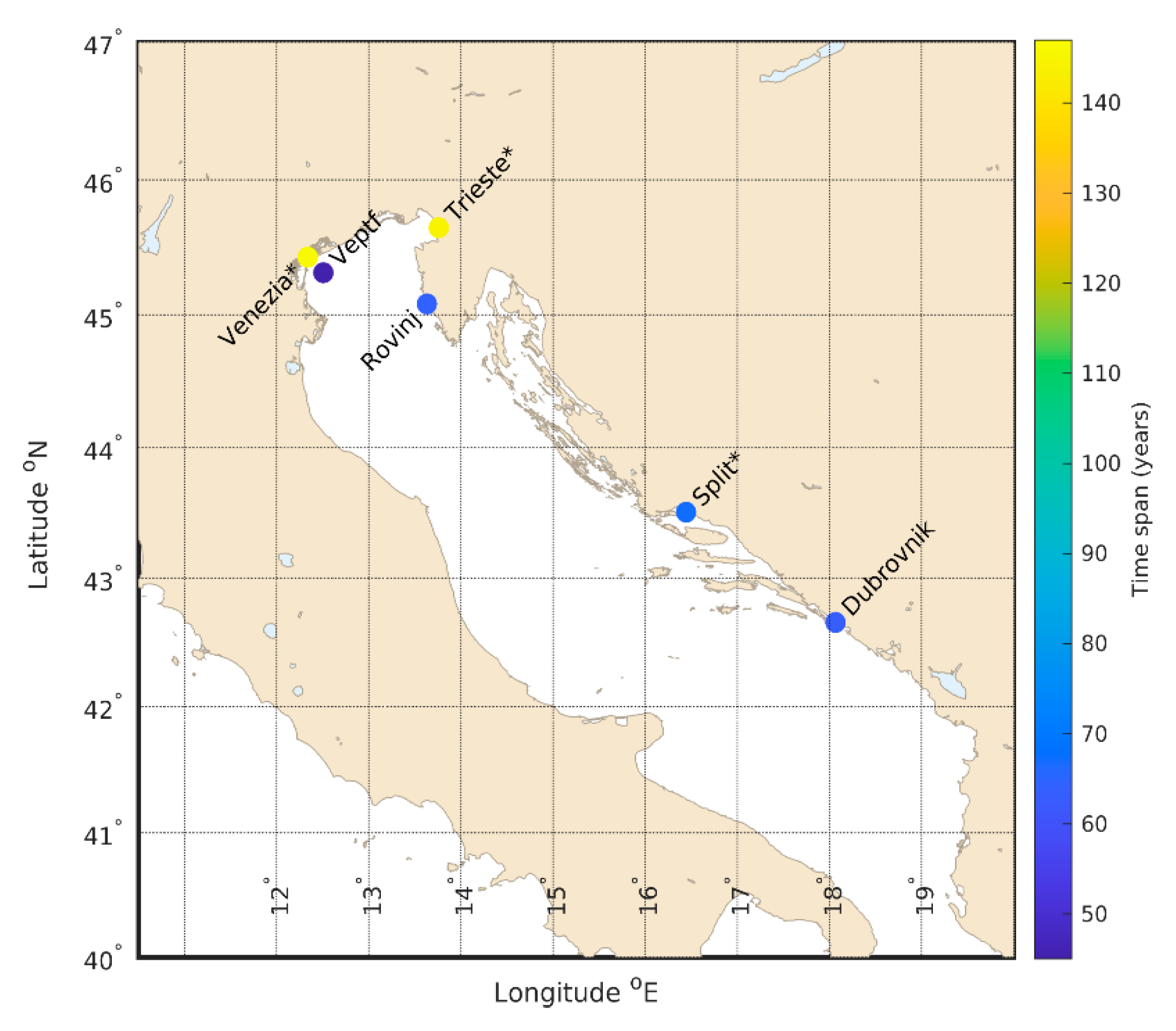
| Location | TG Name | Lat (° N) | Long (° E) | Data (%) | Time Span (Years) | Record Length (Years) |
|---|---|---|---|---|---|---|
| Venice | VENEZIA * | 45°25′51.45″ | 12°20′13.39″ | 97 | 1872–2018 | 147 |
| Venice off-shore | VEPTF | 45°18′51.29″ | 12°30′29.69″ | 100 | 1974–2018 | 45 |
| Trieste | TRIESTE * | 45°38’50.00″ | 13°45’33.90″ | 89 | 1875–2018 | 145 |
| Rovinj | ROVINJ | 45°05’01.18″ | 13°37’44.86″ | 99 | 1955–2018 | 64 |
| Split | SPLIT * | 43°30’23.88″ | 16°26’18.44″ | 100 | 1952–2018 | 67 |
| Dubrovnik | DUBROVNIK | 42°39’28.40″ | 18°03’38.84″ | 99 | 1956–2018 | 63 |
| CGPS | NGL (mm y−1) | Span (Year) | SONEL (mm y−1) | Span (Year) | ISPRA (mm y−1) | Span (Year) | Pooled Mean (mm y−1) |
|---|---|---|---|---|---|---|---|
| PSAL VENEZIA | −1.70 ± 0.80 | 2014–2020 | − | − | −1.46 ± 0.09 | 2010–2015 | −1.59 ± 0.65 |
| TRIE TRIESTE | −0.52 ± 0.45 | 2003–2020 | 0.20 ± 0.26 | 2003–2013 | − | − | −0.25 ± 0.52 |
| SPLT SPLIT | 0.45 ± 0.68 | 2004–2012 | −0.25 ± 0.34 | 2004–2012 | − | − | 0.10 ± 0.64 |
| DUBR DUBROVNIK | −1.99 ± 0.80 | 2000–2012 | – | – | – | – | −1.83 ± 0.70 1 |
| DUB2 DUBROVNIK | −1.94 ± 0.89 | 2012–2020 | – | – | – | – |
| Location | LIP | LIPcov 2 | GPS 3 | ||||
|---|---|---|---|---|---|---|---|
| VENEZIA | 4.16 ± 1.71 | 6.08 ± 2.08 | 3.29 ± 0.82 | −1.93 ± 0.79 | −0.94 ± 0.42 | −1.01 ± 0.42 | −1.59 ± 0.65 |
| VEPTF | 4.17 ± 1.73 | 6.44 ± 2.07 | 3.83 ± 0.81 | −2.27 ± 0.81 | −1.46 ± 0.48 | −1.52 ± 0.48 | - |
| TRIESTE | 4.51 ± 1.84 | 4.49 ± 1.98 | 2.40 ± 0.74 | 0.02 ± 0.71 | −0.05 ± 0.37 | 0.23 ± 0.37 | −0.25 ± 0.52 |
| ROVINJ | 4.09 ± 1.85 | 1.91 ± 2.04 | 1.61 ± 0.73 | 2.18 ± 1.17 | 0.73 ± 0.40 | 0.60 ± 0.40 | - |
| SPLIT | 4.44 ± 1.57 | 4.15 ± 1.87 | 2.45 ± 0.72 | 0.29 ± 0.70 | −0.10 ± 0.37 | 0.11 ± 0.37 | 0.10 ± 0.64 |
| DUBROVNIK | 4.01 ± 1.42 | 4.67 ± 1.70 | 2.80 ± 0.63 | −0.66 ± 0.62 | −0.46 ± 0.51 | −0.69 ± 0.51 | - |
| Pooled mean | 4.23 ± 1.69 | 4.62 ± 1.96 | 2.73 ± 0.75 | −0.40 ± 0.82 | −0.38 ± 0.43 | −0.38 ± 0.43 | −0.58 ± 0.60 |
| Location | LIP | LIPcov | GPS | ||||
|---|---|---|---|---|---|---|---|
| VENEZIA | 4.47 ± 2.07 | 6.08 ± 2.08 | 3.29 ± 0.82 | −1.61 ± 0.91 | −1.02 ± 0.41 | −0.70 ± 0.41 | −1.59 ± 0.65 |
| VEPTF | 4.47 ± 2.07 | 6.44 ± 2.07 | 3.83 ± 0.81 | −1.97 ± 0.93 | −1.54 ± 0.47 | −1.21 ± 0.47 | − |
| TRIESTE | 3.42 ± 1.78 | 4.49 ± 1.98 | 2.40 ± 0.74 | −1.07 ± 0.74 | −0.14 ± 0.36 | −0.86 ± 0.36 | −0.25 ± 0.52 |
| ROVINJ | 4.37 ± 1.86 | 1.91 ± 2.04 | 1.61 ± 0.73 | 2.46 ± 1.04 | 0.65 ± 0.39 | 0.87 ± 0.39 | − |
| SPLIT | 4.15 ± 1.48 | 4.15 ± 1.87 | 2.45 ± 0.72 | −0.00 ± 0.76 | −0.18 ± 0.36 | −0.17 ± 0.36 | 0.10 ± 0.64 |
| DUBROVNIK | 3.98 ± 1.45 | 4.67 ± 1.70 | 2.80 ± 0.63 | −0.69 ± 0.70 | −0.55 ± 0.50 | −0.71 ± 0.50 | − |
| Pooled mean | 4.14 ± 1.80 | 4.62 ± 1.96 | 2.73 ± 0.75 | −0.48 ± 0.85 | −0.46 ± 0.42 | −0.46 ± 0.42 | −0.58 ± 0.60 |
| Dataset | GPS-LIP | GPS-LIPcov | |
|---|---|---|---|
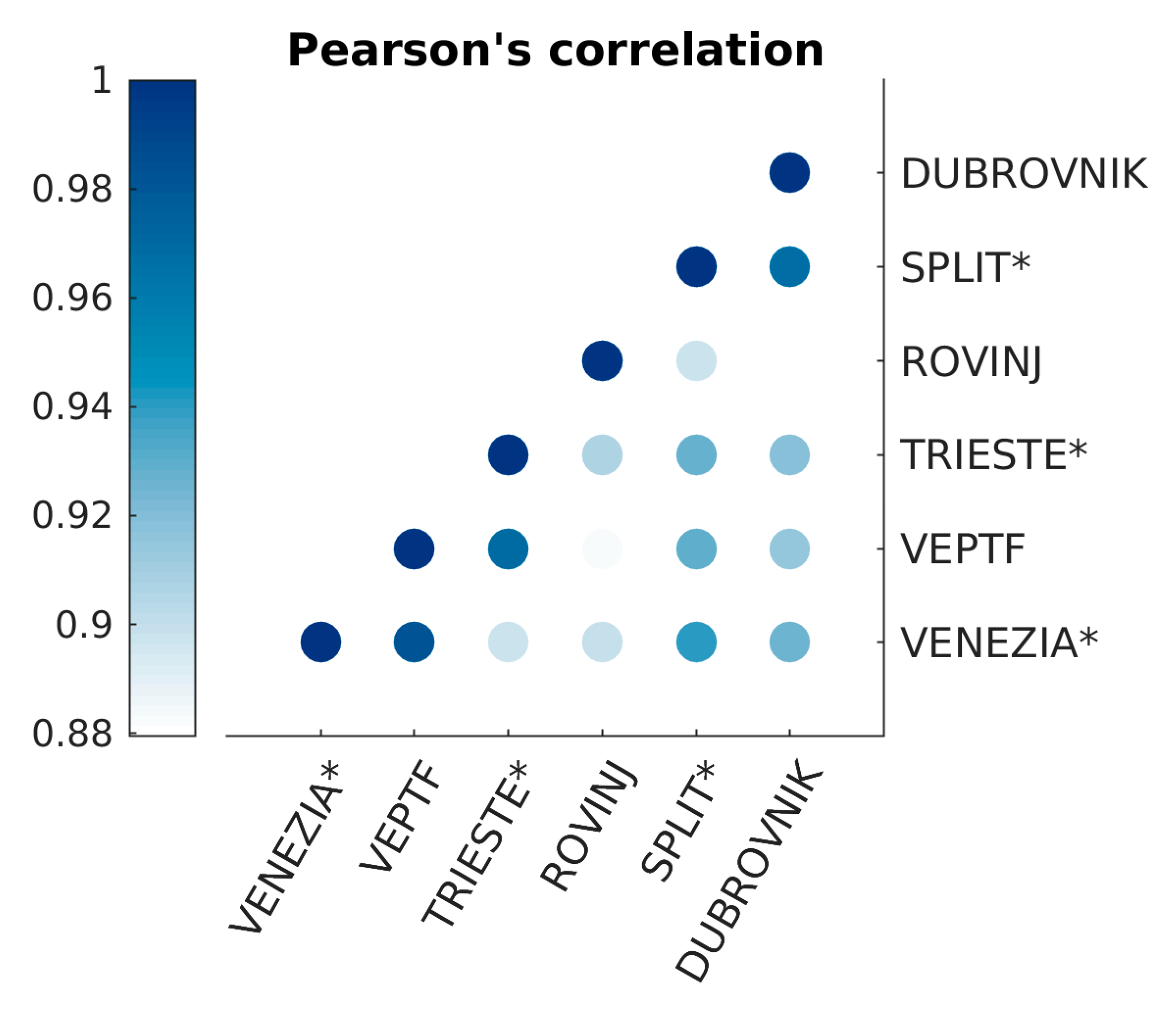
| C3S | 0.274 | 0.409 | 0.435 |
| SLCCI | 0.477 | 0.372 | 0.642 |
| Location | LIP | LIPcov | GPS | ||||
|---|---|---|---|---|---|---|---|
| VENEZIA | 3.36 ± 1.45 | 5.15 ± 1.73 | 3.26 ± 0.73 | −1.79 ± 0.65 | −0.83 ± 0.39 | −0.93 ± 0.39 | −1.59 ± 0.65 |
| VEPTF | 3.38 ± 1.46 | 5.50 ± 1.73 | 3.78 ± 0.73 | −2.12 ± 0.67 | −1.33 ± 0.47 | −1.41 ± 0.47 | − |
| TRIESTE | 3.75 ± 1.58 | 3.56 ± 1.66 | 2.30 ± 0.67 | 0.18 ± 0.60 | 0.13 ± 0.33 | 0.42 ± 0.33 | −0.25 ± 0.52 |
| ROVINJ | 3.33 ± 1.58 | 1.03 ± 1.85 | 1.36 ± 0.71 | 2.30 ± 1.06 | 1.06 ± 0.37 | 0.93 ± 0.37 | − |
| SPLIT | 3.60 ± 1.36 | 2.92 ± 1.65 | 2.20 ± 0.66 | 0.68 ± 0.63 | 0.23 ± 0.33 | 0.37 ± 0.33 | 0.10 ± 0.64 |
| DUBROVNIK | 3.34 ± 1.22 | 3.79 ± 1.48 | 2.69 ± 0.58 | −0.45 ± 0.55 | −0.29 ± 0.46 | −0.41 ± 0.46 | − |
| Pooled mean | 3.46 ± 1.45 | 3.66 ± 1.69 | 2.60 ± 0.68 | −0.20 ± 0.71 | −0.17 ± 0.40 | −0.17 ± 0.40 | −0.58 ± 0.60 |
| LIP | LIPcov | ||||||||
|---|---|---|---|---|---|---|---|---|---|
| Location | 2018 1 | 2015 | diff | 2018 | 2015 | diff | 2018 | 2015 | diff |
| VENEZIA | −1.79 | −1.93 | 0.14 | −0.83 | −0.94 | 0.11 | −0.93 | −1.01 | 0.08 |
| VEPTF | −2.12 | −2.27 | 0.15 | −1.33 | −1.46 | 0.13 | −1.41 | −1.52 | 0.11 |
| TRIESTE | 0.18 | 0.02 | 0.16 | 0.13 | −0.05 | 0.18 | 0.42 | 0.23 | 0.19 |
| ROVINJ | 2.30 | 2.18 | 0.12 | 1.06 | 0.73 | 0.33 | 0.93 | 0.60 | 0.33 |
| SPLIT | 0.68 | 0.29 | 0.39 | 0.23 | −0.10 | 0.33 | 0.37 | 0.11 | 0.26 |
| DUBROVNIK | −0.45 | −0.66 | 0.21 | −0.29 | −0.46 | 0.17 | −0.41 | −0.69 | 0.28 |
| Location | |
|---|---|
| VENEZIA * | 2.33 ± 0.83 |
| VEPTF | 2.37 ± 0.86 |
| TRIESTE * | 2.71 ± 0.75 |
| ROVINJ | 2.29 ± 0.80 |
| SPLIT * | 2.57 ± 0.74 |
| DUBROVNIK | 2.28 ± 0.74 |
| Pooled mean | 2.43 ± 0.80 |
| Sample mean | 2.43 ± 0.18 |
Publisher’s Note: MDPI stays neutral with regard to jurisdictional claims in published maps and institutional affiliations. |
© 2020 by the authors. Licensee MDPI, Basel, Switzerland. This article is an open access article distributed under the terms and conditions of the Creative Commons Attribution (CC BY) license (http://creativecommons.org/licenses/by/4.0/).
Share and Cite
De Biasio, F.; Baldin, G.; Vignudelli, S. Revisiting Vertical Land Motion and Sea Level Trends in the Northeastern Adriatic Sea Using Satellite Altimetry and Tide Gauge Data. J. Mar. Sci. Eng. 2020, 8, 949. https://doi.org/10.3390/jmse8110949
De Biasio F, Baldin G, Vignudelli S. Revisiting Vertical Land Motion and Sea Level Trends in the Northeastern Adriatic Sea Using Satellite Altimetry and Tide Gauge Data. Journal of Marine Science and Engineering. 2020; 8(11):949. https://doi.org/10.3390/jmse8110949
Chicago/Turabian StyleDe Biasio, Francesco, Giorgio Baldin, and Stefano Vignudelli. 2020. "Revisiting Vertical Land Motion and Sea Level Trends in the Northeastern Adriatic Sea Using Satellite Altimetry and Tide Gauge Data" Journal of Marine Science and Engineering 8, no. 11: 949. https://doi.org/10.3390/jmse8110949
APA StyleDe Biasio, F., Baldin, G., & Vignudelli, S. (2020). Revisiting Vertical Land Motion and Sea Level Trends in the Northeastern Adriatic Sea Using Satellite Altimetry and Tide Gauge Data. Journal of Marine Science and Engineering, 8(11), 949. https://doi.org/10.3390/jmse8110949