Evaluating the Sensor-Equipped Autonomous Surface Vehicle C-Worker 4 as a Tool for Identifying Coastal Ocean Acidification and Changes in Carbonate Chemistry

Abstract

The interface between land and sea is a key environment for biogeochemical carbon cycling, yet these dynamic environments are traditionally under sampled. Logistical limitations have historically precluded a comprehensive understanding of coastal zone processes, including ocean acidification. Using sensors on autonomous platforms is a promising approach to enhance data collection in these environments. Here, we evaluate the use of an autonomous surface vehicle (ASV), the C-Worker 4 (CW4), equipped with pH and pCO₂ sensors and with the capacity to mount additional sensors for up to 10 other parameters, for the collection of high-resolution data in shallow coastal environments. We deployed the CW4 on two occasions in Belizean coastal waters for 2.5 and 4 days, demonstrating its capability for high-resolution spatial mapping of surface coastal biogeochemistry. This enabled the characterisation of small-scale variability and the identification of sources of low pH/high pCO₂ waters as well as identifying potential controls on coastal pH. We demonstrated the capabilities of the CW4 in both pre-planned “autonomous” mission mode and remote “manually” operated mode. After documenting platform behaviour, we provide recommendations for further usage, such as the ideal mode of operation for better quality pH data, e.g., using constant speed. The CW4 has a high power supply capacity, which permits the deployment of multiple sensors sampling concurrently, a shallow draught, and is highly controllable and manoeuvrable. This makes it a highly suitable tool for observing and characterising the carbonate system alongside identifying potential drivers and controls in shallow coastal regions.

1. Introduction

The ocean has taken up approximately 25% of all CO₂ emitted to the atmosphere by human activity [1], resulting in a decrease in ocean pH of 0.1 units since 1750 [2], a phenomenon known as ocean acidification. Oceanic uptake is directly proportional to the gradient in pCO₂ between the surface ocean and the atmosphere [3]. Current models indicate that projected emission rates will cause 1000 µatm pCO₂ to be reached by 2100, with ocean pH decreasing by a further 0.3 units [4]. However, pCO₂ values over 1000 µatm have already been recorded in coastal environments (e.g., [5]). Traditionally it was thought that ocean acidification was solely due to the increasing flux of atmospheric CO₂ into the ocean [6], but the importance of other processes on coastal pH, such as eutrophication and microbial respiration, are now being recognised [5,7,8]. Eutrophication leads to an increase in organic matter, the heterotrophic degradation of which results in the production of CO₂ and, therefore, acidification [9]. It is becoming increasingly apparent that ocean acidification driven by the uptake of anthropogenic CO₂ from the atmosphere alone is mainly an open ocean syndrome and that coastal ocean acidification has far more complex causes [6]. Therefore, full characterisation of coastal ocean acidification requires highly resolved measurements of multiple parameters over both spatial and temporal scales [10,11], with autonomous platforms providing a scalable solution to this challenge [10].

Coastal oceans support both biogeochemically and structurally complex ecosystems [12], which account for 14–30% of the ocean’s primary production [13]. They are often dominated by benthic ecosystems (e.g., corals, seagrass, mangroves, oyster reefs), which can impact (and be impacted by) both chemical and physical environmental conditions [14]. Presently, we do not possess the capability to provide a comprehensive overview, and the relative significance, of the processes controlling pH in coastal waters. This is due to a combination of logistical, technological, and economic factors. Many coastal regions are inaccessible to manned research vessels [10] due to shallow bathymetry and features such as rocky outcrops, reefs, sandbanks, and calving glaciers as well as health hazards such as sewage outflows. Research vessels also require a large support crew, and are therefore costly to operate, and can have restricted availability and work areas [15], as well as often being skewed to summer months [10]. The logistical limitations of discrete bottle sampling from manned research vessels or from shore-based platforms are a barrier to attaining the large spatial and temporal data coverage required in many regions. The development and implementation of new technology-based approaches will be key to overcoming these challenges [11].

Recent advances in autonomous platform technologies have the potential to improve spatial and temporal coverage of oceanographic observations, while reducing operating costs [10]. Autonomous technologies evolve for different requirements—moorings, for example, can measure temporal scales from hours to decades, but only measure on the order of meters, while profiling floats can measure from km to global scales [10]. Recent advancements have seen both gliders [16] and profiling floats [17] being used to monitor ocean acidification using pH sensors; however, both profiling floats and gliders usage can be limited by water depth, as they are best fitted to sample depths >20 m. They are also driven by buoyancy and currents, so are not the best platforms to sample large spatial scales in short periods of time. To sample coastal environments appropriately at the relevant scales, which are very dynamic and present more sub-mesoscale features than the open ocean, there is a greater need for faster, high-resolution temporal and spatial sampling. The shallow draft, compact size, and increased manoeuvrability of Autonomous Surface Vehicles (ASVs) enable them to operate in (often inaccessible) shallow waters and access both riverine and coastal marine environments [18], including narrow channels [11], potentially making ASVs a very useful platform for monitoring coastal ocean acidification.

Despite ASVs having been in development for over two decades [18], their use in oceanographic research is not yet widespread (e.g., [11,15,19,20,21,22,23,24,25,26]), in particular for observations of coastal carbonate chemistry. Studies have successfully demonstrated pCO₂ sensors mounted on Wave Glider [27], Saildrone [22], and ChemYak [11] and more recent advancements deploying both pH and pCO₂ sensors on Wave Glider [28,29] and Saildrone [29] ASVs. Measuring pH and pCO₂ simultaneously allows Dissolved Inorganic Carbon (DIC) and Total Alkalinity (TA) to be calculated [30], and therefore, processes that may be controlling regional carbonate chemistry and coastal ocean acidification may be identified. While pH and pCO₂ exhibit a strong co-variance [10], they are currently the only two carbonate parameters that can be measured with “off-the-shelf” sensors, though DIC [31] and TA [32] sensors are currently in development. The ability to integrate calibrated, powered, well-maintained, and commercially available sensors into autonomous vehicles increases our capacity to monitor coastal ocean acidification and biogeochemistry at the relevant and necessary scales. The type of research will shape the requirements for the ASV type; for longer missions, the ability to recharge batteries at sea is needed, e.g., Wave Glider and Saildrone’s use of solar panels [29], but power availability can limit both sensor capacity and sampling frequency. In coastal environments, where endurance is not a priority given that the vehicles can be easily refuelled, a vehicle that is powered by diesel or petrol (e.g., ChemYak [11]) may be more desirable since it allows increased sensor load and improved resolution, as sampling frequency does not need to be limited to save power. Furthermore, the aforementioned solar powered ASVs are not capable of sampling in very shallow coastal regions with depths of 5 m or less.

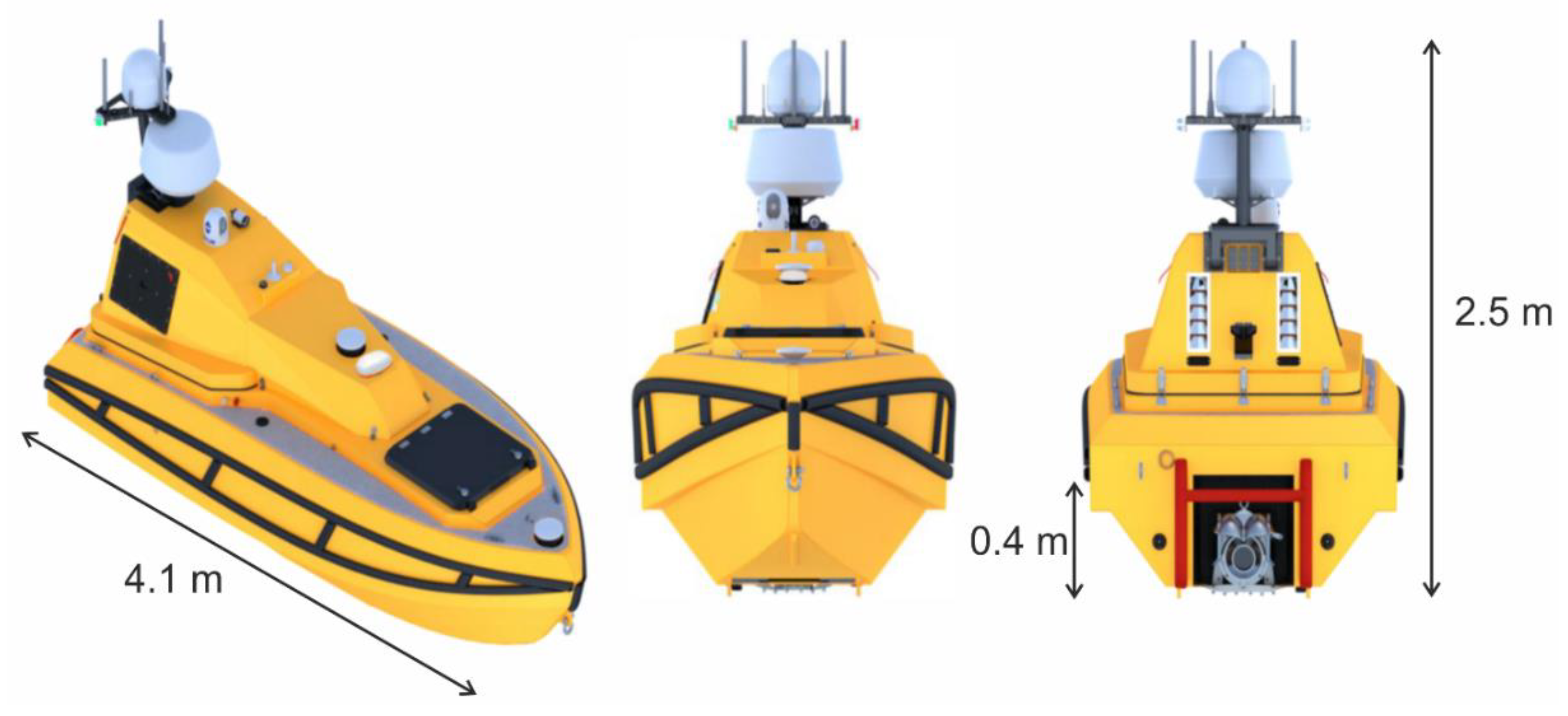
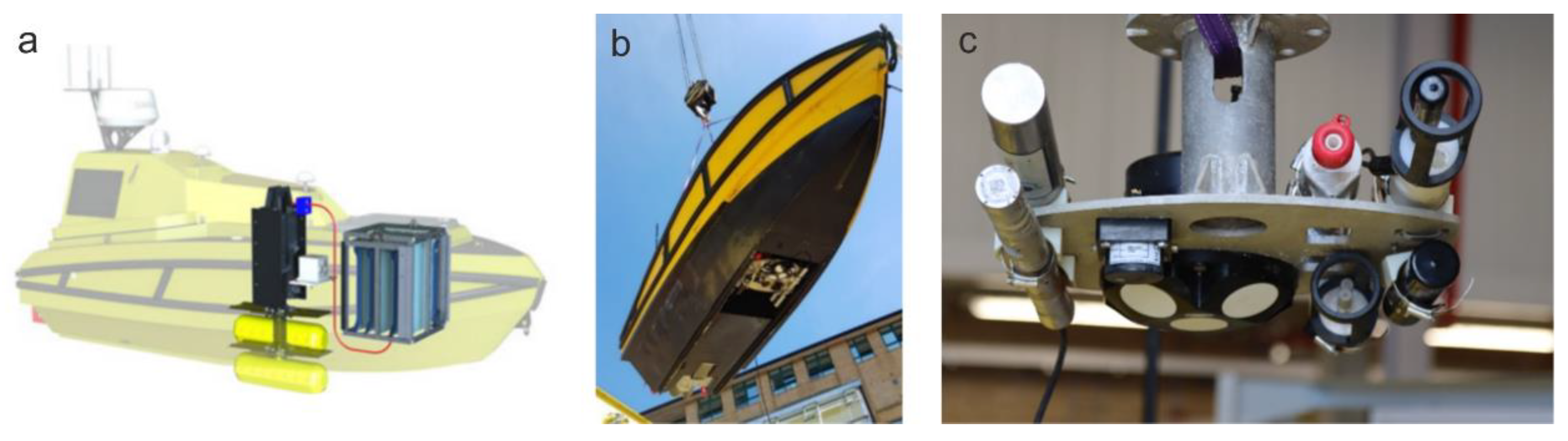
In this study, we assess the capabilities of the ASV C-Worker 4 (CW4) equipped with off-the-shelf sensors as a tool for investigating coastal ocean acidification in shallow environments. The CW4 was deployed in Belize, on the Caribbean coast of Central America, under the Commonwealth Marine Economies Programme (CMEP) as part of the Containerised Autonomous Marine Environmental Laboratory (CAMEL) facility [33]. The CAMEL was developed for use in small island developing states to allow mapping and monitoring of local marine environments as part of CMEP partnership between the UK National Oceanography Centre, the UK Hydrographic Office, and the Centre for Environment, Fisheries and Aquatic Science. Belize’s coastal zone was considered an appropriately challenging test area owing to its barrier reef, associated network of cayes (islands) and shallow lagoons, alongside a diverse array of habitats (seagrass, mangroves, and coral reefs). The low-resolution bathymetry in this region, making the use of research vessels challenging, provided another benefit to using this platform. Furthermore, Belize is undergoing coastal development and significant land use changes with likely associated shifts in the biogeochemistry of freshwater discharge, contributing to the dynamic and heterogeneous nature of carbonate chemistry over its coastal shelf. The capabilities of the CW4 were demonstrated by conducting cross-shore transects from river mouth to reef, identifying spatial changes in carbonate chemistry and potential drivers using concomitant biogeochemical parameters. A series of tests were conducted to assess this platform and to provide further recommendations to collect quality OA and biogeochemical data.

2. Materials and Methods

2.1. The Vehicle—C Worker 4

The CW4, developed by L3 Harris, is a 4.1 m long, 2.5 m high, autonomous surface vehicle with a draft of 0.4 m and mass of 980 kg (maximum, when fully laden) (Figure 1). The hull is divided into two main compartments: an air-conditioned fore compartment (the payload bay), which houses the payload computers, and an aft compartment that houses the engine. The vehicle’s propulsion system is a 30-horsepower diesel inboard engine coupled with a centrifugal clutch shaft, which is connected to a water jet. The diesel exhaust is situated at the back of the vehicle and sits above the water line; therefore, it should not affect water chemistry. On a full tank (~100 L), the CW4 has a maximum endurance of 48 h, but it can be re-fuelled while in the water, minimising launch and recovery operations. It is designed to operate in waters up to a sea state of 3. When set on a mission, the CW4 can be programmed to a desired throttle capacity or speed of up to 7 knots.

The CW4 can be operated in 2 main modes: (1) by remote control or (2) set on pre-planned missions, it can also hover on a waypoint or follow a target (e.g., another vessel). Missions are set by plotting a series of waypoints to create a transect; when the vehicle reaches the last waypoint, it will move onto the next mission or pause and wait for the next instruction. The control station communicates with the vehicle via a mesh radio link or WiFi. Radio control distance range is dependent on antenna height, and whether the vehicle is in sight of the antenna. During our field trials, we have successfully controlled the vehicle from 10 km distance. Visibility and identification of the CW4 by nearby vessels is provided by an Automatic Identification System (AIS) equipped on the vehicle. Remote control operation is enabled by a 180° day camera and a thermal imaging camera installed on the CW4 which together provide the operator with a real-time view from the vehicle’s perspective. The CW4 is also fitted with a radar.

Personnel operating the CW4 are required to pass training courses provided by the vehicle manufacturer and hold a RYA (Royal Yachting Association) powerboat certificate and VHF radio license. An additional person is required as a watch keeper. On-water operation of the CW4 can therefore be achieved with two trained individuals. Situational awareness includes the radar display, AIS information, video feeds, and water depth which are supported where necessary by line of sight vision. However, the CW4 is not currently equipped with collision avoidance technology; therefore, avoidance actions require intervention by a pilot.

The vehicle’s payload computer and installed sensors are powered by a 240 V 50 Hz inverter. Sensors are mounted to a plate (Figure 2c), which is lowered from the hull of the vehicle when in operation, and housed inside the hull when not in use (Figure 2b). The ability to raise and lower the payload prevents damage to sensors when moving the CW4 in and out of the water and in shallow regions. When the vehicle is stationary, the sensors sit at 0.65 m depth and when in motion, the sensors sit at ~0.55 m.

2.2. Sensor Payload

The payload we deployed comprises sensors for conductivity, temperature, depth (CTD), dissolved oxygen (DO), pCO₂, pH, nitrate, chlorophyll fluorescence, Coloured Dissolved Organic Matter (CDOM), Turbidity, Dissolved Organic Carbon (DOC), and current profiling (

Table 1. Sensors mounted on CW4. There are two RBR Concerto³ loggers mounted on the CW4, with different sensors attached, differentiated by numbers in brackets.

Sensor Parameter	Sensor Manufacturer (and Logger)	Method of Sampling	Sampling Frequency (s)	Factory Accuracy
Conductivity	RBR (on RBR Concerto3 1)	Inductive current and receiver	0.125	±0.003 mS/cm
Temperature		Aged glass thermistors		±0.002 °C
Sensor Depth		–		±0.05%
Dissolved O2 (DO)	RBR, normal foil (on RBR Concerto3 2)	Optically dynamic luminescence quenching	0.5	±8 µM
Temperature	RBR (on RBR Concerto3 2)	Aged glass thermistors		±0.002 °C
pH	Idronaut (on RBR Concerto3 2)	Glass membrane pH electrode		0.01
pCO2	Turner C-sense (on RBR Concerto3 2)	non-dispersive infrared (NDIR) detector		±3% full scale (1000 ppm)
Nitrate	Seabird SUNA V2	Optical UV	0.67	±8 µM
Chlorophyll	Sea-Bird WET Labs EcoPuck Triplet Optical Sensor	Fluorescence (695 nm)	1.06	±0.025 µg/L
Coloured Dissolved Organic Matter (CDOM)		Fluorescence (460 nm)		±0.28 ppb
Optical Backscatter		Optical Backscatter (700 nm)		±0.003 m−1
Dissolved Organic Carbon (DOC)	S::can Spectro::lyserTM	UV–vis spectrometry (190–750 nm)	180	±2%
Turbidity
Total Organic Carbon (TOC)
Current profiling	Nortek Signature 500 Acoustic Doppler current profiler (ADCP)	Acoustic Doppler	1	±0.1 cm/s (velocity resolution)

) (Figure 2). Depending on the power and memory capacity, sensors can be set to self-log, or connected to an on-board computer (Figure 2a). Connection to the computer is desirable as data are stored in real-time on to the computer’s hard drive as well as on the sensor (depending on sensor capability). Given that the operator can connect to the on-board computer, the operator can receive a live data feed or even transfer data throughout the mission. This allows the diagnosis (and timely fix) of potential issues on the data collection as well as to conduct adaptive sampling. Results from the Nortek Signature 500 current profiler (ADCP) are not shown as it is beyond the scope of this paper, but it does provide an additional source of water depth and GPS location if the CW4 depth sounder or GPS location were to fail.

2.3. Study Site and Deployment

The Belize River, which drains the largest catchment in the country [35], discharges north of Belize City, with the barrier reef located ~15 km off the coast from that point. Our study area (17° to 17.6° N and 88° to 88.3° W) extends from the Belize River mouth to the barrier reef near St George’s Caye and south of the main shipping channel to Southern Long Caye, and encompasses much of the outflow region of the Belize River (Figure 3), as predicted from composite satellite imagery of the turbidity and local knowledge. The influence of the Belize River will vary with season, tending to head straight east or south around Belize City then east, depending on both wind direction and freshwater volume. In 2019, we wanted to sample during the wet season when the influence of the river would be greatest; however, Belize was unfortunately experiencing a drought during our field campaign. The study area contains a diverse array of habitats including seagrass, mangroves, and coral reef, with the depth of the study area less than 1 m in many places.

In November 2018, the inaugural deployment of the CAMEL and CW4 took place in Belize. We conducted 2.5 days of sampling (24–26 November 2018) around Belize City and along the Belize Barrier Reef down the barrier reef to Southern Long Caye (Figure 3). On return to Belize in 2019, over 4 days of operation (17–20 October 2019) the CW4 conducted 4 pre-planned transects totalling 181 km. In 2018, the CW4 was deployed with a biogeochemical payload, measuring CTD, DO, pCO₂, chlorophyll, CDOM, optical backscatter, turbidity, DOC, TOC, and currents. In 2019, the CW4 was deployed with nitrate and pH sensors in addition to the 2018 setup. To better characterise the platform’s behaviour in 2019, we designed specific transects and conducted a number of tests: (1) to assess line following ability, the CW-4 was tasked to follow a transect with multiple right angle turns (Transect 1) in autonomous mode; (2) to test the effect of speed on sensor performance and noise, we evaluated sensor data stability under a varying range of vehicle speeds, from 0 to 5 kts (Transect 4).

The CW4 was set on pre-planned missions, where manual control was only necessary in shallow areas, such as in the river mouth, where depth decreased to ~0.5 m. During pre-planned missions, the CW4′s speed was kept between 4.0 and 5.5 kts. As agreed with the Belize Port Authority, the CW4 remained in sight of the operator at all times, from a 38 ft fibre glass support vessel. Discrete water samples were additionally taken from the support vessel.

2.4. Sensor Data Processing

All sensor data were processed using pre-deployment manufacturer calibrations according to recommended best practice. pH, DO, CTD, chlorophyll fluorescence, CDOM, optical backscatter, and nitrate data were initially smoothed by taking an 11-point moving median to remove inherent noise created by high-resolution sampling and sensor response time. Spectrolyser data were not smoothed due to the lower sampling frequency of the data, a data point every 3 min, and was factory calibrated using ana::pro software.

3. Results and Discussion

3.1. Endurance, Range, and Resolution

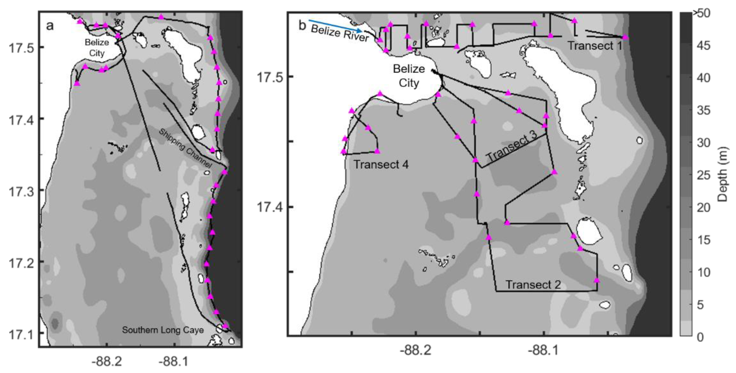
In 2019, the CW4 collected data over 181 km, taking 25 h to complete the four transects. At the average speed employed of 5 knots, a transect of the entire Belizean coastline could be surveyed in approximately 40 h, which is within the maximum endurance of the CW4. For longer missions, the vehicle’s range can be extended by rendezvous and refuelling with a support vessel, as the CW4′s diesel engine can easily be refuelled at sea. For a small country such as Belize, or island states, the vehicle’s range and endurance would facilitate comprehensive surveys over meaningful spatial scales in a matter of days. Based on the settings used on our field deployments (vehicle speed and sensor resolution), the CW4 collected, on average per km, around 900 measurements of pH and pCO₂ and about 3500 measurements of temperature, salinity, and depth. The lowest frequency of measurements was generated by the spectrolyser, which collected between 2 and 3 data points per km. In comparison, during the 2019 deployment, we were able to collect a maximum of 39 discrete water samples (Figure 3) limited by the time and effort required to collect, preserve and store samples according to best practices (e.g., [30,36]) (a sampling frequency ~0.22 samples per km). This illustrates the pronounced advantage in resolving spatial and temporal variation using a sensor-based approach. Analysis of these samples has been delayed due to the COVID-19 pandemic and we plan to present these data in a future paper focused on evaluating sensor performance as opposed to the focus on vessel performance and operational experience reported here.

We successfully received a live data feed from the CW4 at all times that the vehicle was in range. We found the bandwidth of the mesh radio link between the support vessel and the CW4 sufficient for receipt of the navigational data and camera feed, and also could accommodate the remote desktop feed from the payload PC. Access to real-time sensor data is helpful as it provides confidence in the validity of the data being collected and affords the option to revise the vehicle’s course during a deployment in response to the conditions encountered. It also enables optimisation of the sensor setup in real-time, which is likely to be of particular utility for SideScan sonar or multibeam echo sounders. However, the bandwidth of the datalink was barely satisfactory for the download of the datasets. Thus, datasets from each deployment were generally recovered via a wired Ethernet connection when the CW4 was docked.

3.2. Navigation: Course Holding and Correction

A primary physical barrier in coastal environments is the shallow and/or shifting bathymetry, which can be prohibitive to manned vessels. Additionally, autonomous vehicles possess sophisticated navigation and position control systems that can be superior to manned vessels of similar size and draft. ASVs, such as the CW4, often have the ability to accurately navigate course tracks autonomously and repeat course tracks over sequential missions, in order to monitor environmental changes at the same location through time.

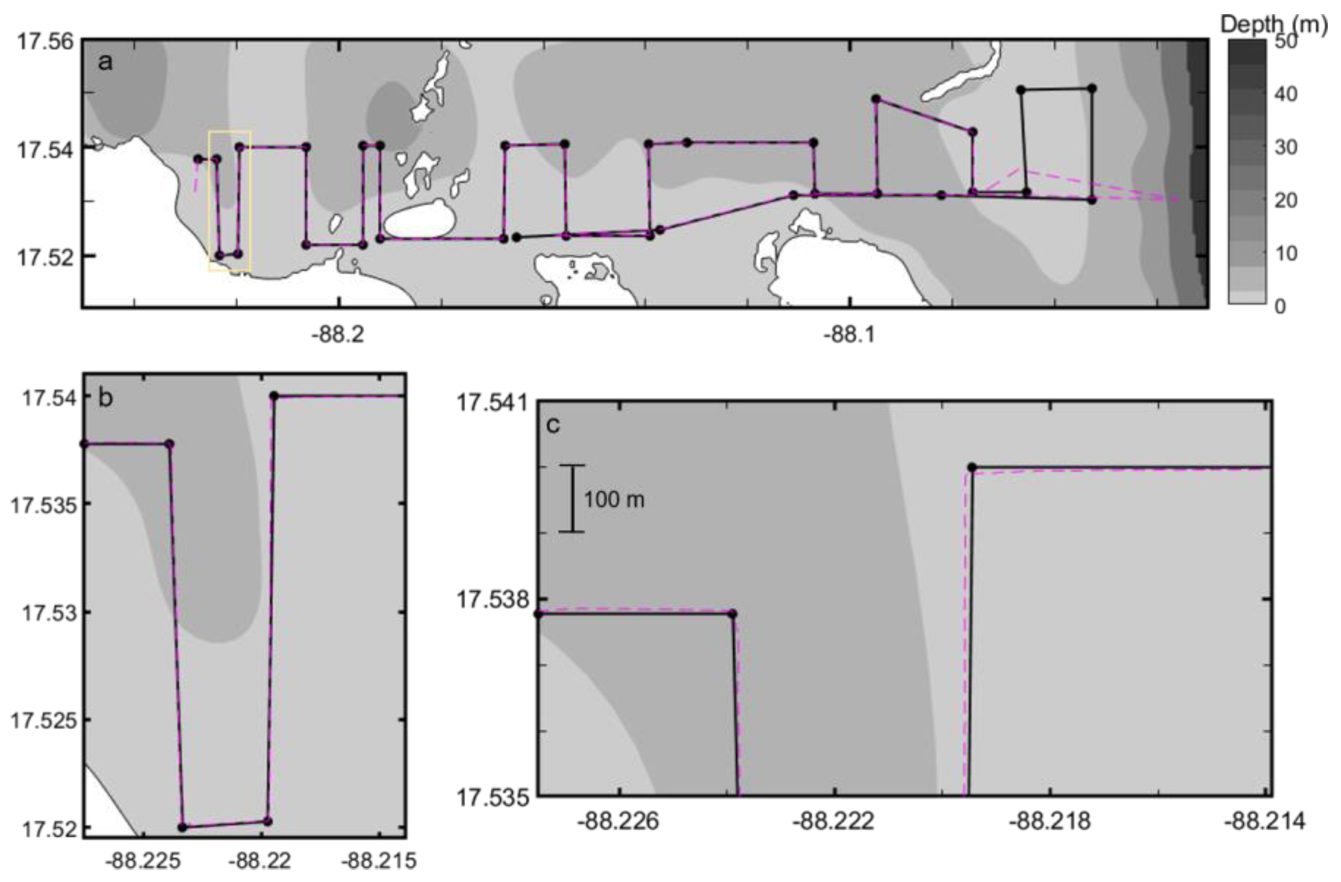
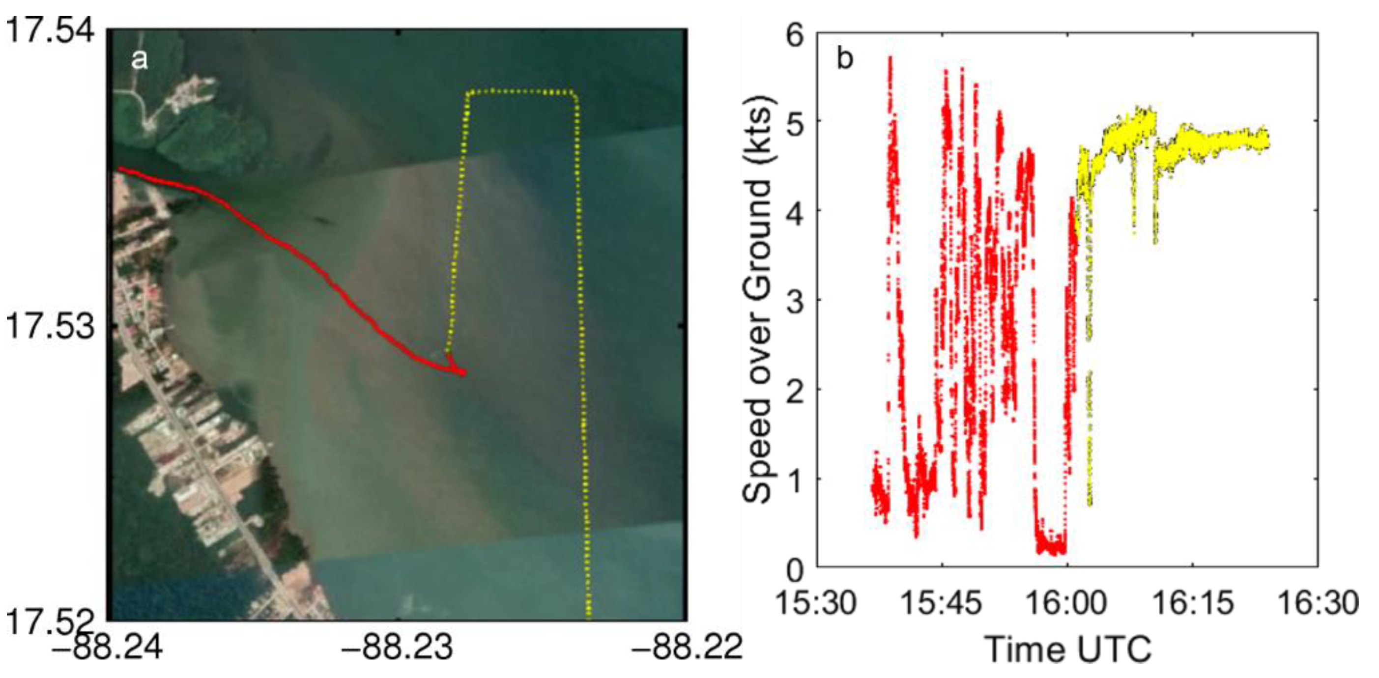
In order to understand its capability to hold course, we tasked the CW-4 to follow a transect with multiple turns. The CW4 successfully navigated all of the pre-planned missions during our two field campaigns. Deviations (5–34 m) from the course track were observed when carrying out 90-degree turns (Figure 4). It is likely that this deviation was caused by setting a fixed mission throttle, thereby preventing the vehicle from reducing its speed in order to perform a controlled turn. The southerly wind may have played a role in the course deviation, as the largest deviations were consistently recorded when turning from a southern heading to east bound, and both wind and current are known to affect the path of a vehicle [37]; however, maximum wind speed was 4.02 m/s [38], which would unlikely be strong enough to have a noticeable effect. Transects are set by programming a series of waypoints and when the vehicle comes within 3 m of a waypoint, it moves to the next. We defined waypoints only at corners; therefore, increasing the frequency of waypoints between two corners would potentially improve the transect following accuracy. Increasing the number of waypoints would also be particularly beneficial in shallow regions where course deviation may result in grounding and/or damage to the vehicle and local ecosystems, or in areas without accurate bathymetric information. While the CW4 has been shown to deviate from the transect, as the vehicle is constantly recording its location (10 Hz), we know the exact location and do not have to interpolate location, as is done by some underwater autonomous technologies.

At the end of Transect 1 (Figure 4a), a shallow sand bank was identified, which was a potential grounding hazard to the vehicle and which required changes to the vessel’s track during the mission. The depth information is available for navigational purposes from the depth sensor mounted to the vessel and situational avoidance requires pilot intervention. Through mission control, the CW4 was given new waypoints to continue navigating and successfully altered its path, continuing on pre-planned mode (Figure 4, pink dashed line). Although the additional two new waypoints were not automatically saved (a limitation of the vehicle control software, thus are not marked on Figure 4), the vessel’s completed track is always stored. The operator receives a live data stream and has the ability to alter the vehicle’s path during the mission. Therefore, this not only allows hazard avoidance but facilitates responsive surveying. This capability to alter the pre-planned mission can provide opportunities to map features of interest that arise, such as low salinity lenses, which could be indicative of a freshwater source and lower pH water. This capability can be particularly useful where there may be multiple freshwater sources, especially if they are previously unknown, such as submarine groundwater discharge points. It can also be used for adaptive sampling, e.g., to inform interesting discrete water sampling locations for other parameters that cannot be measured with sensors.

The CW4 conducted smoother tracks with a more consistent speed when set on a pre-planned mission as opposed to being driven remotely (Figure 5). When set on a mission, a desired throttle or speed is set, creating a steadier track. When driven remotely, speed and direction are controlled by the operator and can therefore, be more variable. The ability to change mode of operation (pre-planned “autonomous” mission vs. remotely “manually” operated) is a useful feature of the CW4: narrow channels can be easily navigated and hazards avoided; and during launch and recovery, it can be driven onto a trailer on a slip way, or easily docked at a pontoon. We controlled CW4 remotely when entering and exiting the Belize River (Figure 5) due to the shallow nature of the river mouth, with the entrance into the river as shallow as 0.5 m, requiring local knowledge of this dynamic area. By having the ability to take control of the vehicle, we were able to safely navigate in and out of the river without damaging the sensor payload.

3.3. Relative Operation Costs

Here, we undertake some simple illustrative calculations around the costs associated with different operating models to determine the possible cost savings associated with using a CW4-type vehicle. Costs are clearly sensitive to the chosen sampling approach, ranging from a remotely operated CW4 with user calibrated sensors through to traditional manual in situ sampling from a vessel (with no autonomous vehicle). For simplicity, we compare two scenarios: (1) the CW4 with a support boat and no sampling, and (2) the same support boat and personnel to manual sampling along the CW track. Assuming that the support boat could undertake 10 stations per day whilst in survey mode (realistically the maximum possible based on our experience), we estimate the cost saving from using the CW4 as being around 25% due to sample analytical costs (~GBP 60–80 per station assuming analytical facilities are available in the region). In practice, the savings would be much larger. Given the coarse resolution of a manual survey, to achieve anything approaching the same spatial and temporal scales as the CW4, a much longer and costly surveying period would be required. An alternative evaluation of the cost savings associated with the CW4 is to compare its operation to using a research vessel. The initial cost of purchasing the CW4 and the sensor suite used is approximately ~GBP 500,000, which is a fraction of the cost of a research vessel and the associated analytical instrumentation required to analyse multiple samples. The operating costs of a research vessel are also much larger, including associated fuel costs. A typical research ship will use ~9000 L fuel per day, while the CW4 used ~30 L/day. Thus, the carbon footprint associated with the science programme is also vastly reduced via usage of the CW4.

3.4. Resolving Carbonate Chemistry

During our trials, we equipped the CW4 with a sensor payload which collects a wide range of parameters, including pH and pCO₂. Having the ability to measure both pCO₂ and pH simultaneously can be used to identify controls on pH variability and track these changes, as it allows the calculation of total alkalinity and DIC. While many models derive total alkalinity from salinity, this linear relationship is not robust in the dynamic coastal environment [39]. Both Wave Glider and Saildrone have successfully collected pH and pCO₂ data simultaneously [28,29]. However, given its long umbilical, the Wave Glider would require more than 7 m of water depth [26] and the Saildrone has a 2.5 m keel [29], which would render both unsuitable for a significant portion of our study area, and in many shallow coastal regions home to ecosystems such as coral reefs and seagrass.

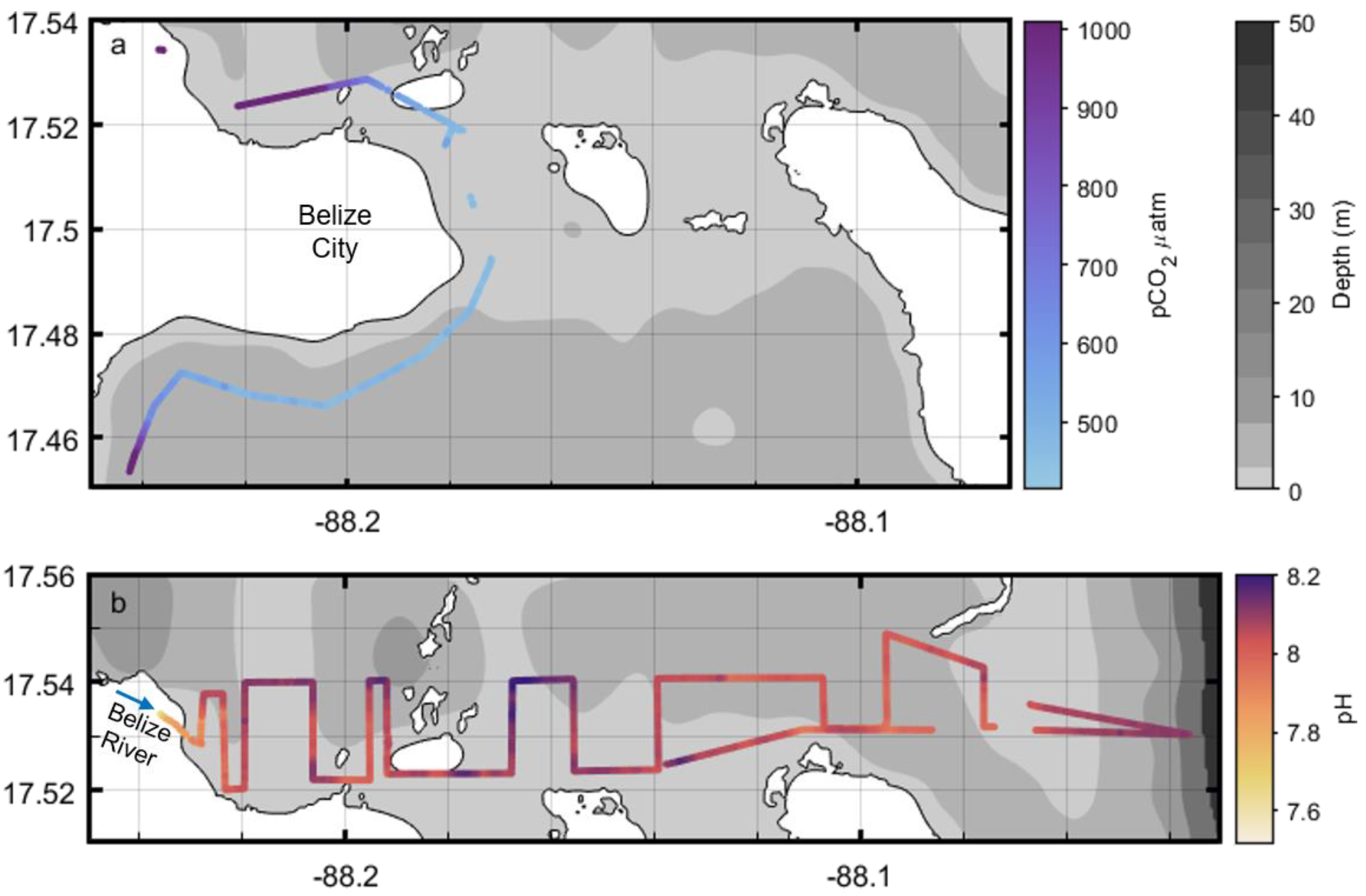
Spatially mapping pH and pCO₂ allows us to identify sources of high pCO₂/low pH water alongside changes in both surface pH and pCO₂ (Figure 6). In 2018, we deployed the CW4 with a Turner C-sense pCO₂ sensor. We found a gradient in pCO₂, with higher concentrations near the Belize River, lower further from the coast, and higher variability around Belize City. The pCO₂ sensor became saturated in the river mouth at 1011 µatm pCO₂, but this is a limitation of the mounted sensor, not of the platform. Increasing the calibrated sensor range would allow us to have a better idea of maximum river pCO₂, but it would decrease sensor accuracy, reducing the ability to identify changes at lower values. For the Turner C-sense, the accuracy is 3% of the total scale. Given the payload capabilities of this platform, two pCO₂ sensors with different ranges (one optimised for low concentrations and one for high) could be mounted to fully cover the dynamic range found in this region.

In 2019, we deployed the CW4 with an Idronaut pH sensor. There was a general increase in pH from the Belize River mouth towards the barrier reef, but fine-scale variability is also apparent. Unfortunately, during the 2019 campaign, the Turner C-sense pCO₂ sensor failed due to damage to the sensor’s membrane, so we were unable to collect concurrent measurements of both sensors. This does not invalidate the usefulness of this platform in collecting carbonate chemistry, as we show during our two field deployments, the vehicle can collect both parameters. Additionally, in pre-deployment testing, we successfully collected both pCO₂ and pH in parallel. During the pre-deployment testing, we identified vehicle interference on the pH measurements when the instrument was connected to the on-board computer, with both increased noise and a shift in pH values identified. We performed a single point calibration in August 2019 of the pH sensor in certified saline Tris buffer while the sensor was both connected to the on-board computer or set to self-logging with the RBRConcerto³. During self-logging, the sensor measured pH within 0.021 of the expected value; a greater offset was identified from the Tris buffer when connected to the on-board computer. The likely theory is there is some form of conducted electromagnetic interference between the sensor and the CW4 when connected to the on-board computer with a RS232 cable. To eliminate the issue for the 2019 deployment, the second RBR Concerto³, to which the DO and pH sensor were attached, was disconnected from the vehicle during each mission so that it was powered from its internal batteries, and logged its data internally. The data were recovered from the sensor at the end of each day. No other sensor exhibited this phenomenon, so all the other sensors logged their data to the payload PC and these data were viewable in real time at the control station.

As expected, the pH sensor identified the Belize River as a source of low pH water with a general increase towards the barrier reef as distance from river mouth increased. However, given the high-resolution surface biogeochemistry mapping capabilities of this platform, we are able to identify fine-scale fluctuations along the transect. The variability recorded in pH is larger than the reported sensor accuracy (Table 1) and while sensor drift can occur, it is likely to be minimal as data collection took place over a few days, with sensor manufacturer Idronaut reporting a drift of 0.05 pH/month, which is significantly less than the range of measurements we observed (Figure 6). Therefore, the resultant datasets are comparable within the same deployment and show that our approach is useful for spatial monitoring of coastal regions and identifying point sources of low pH, high pCO₂ water.

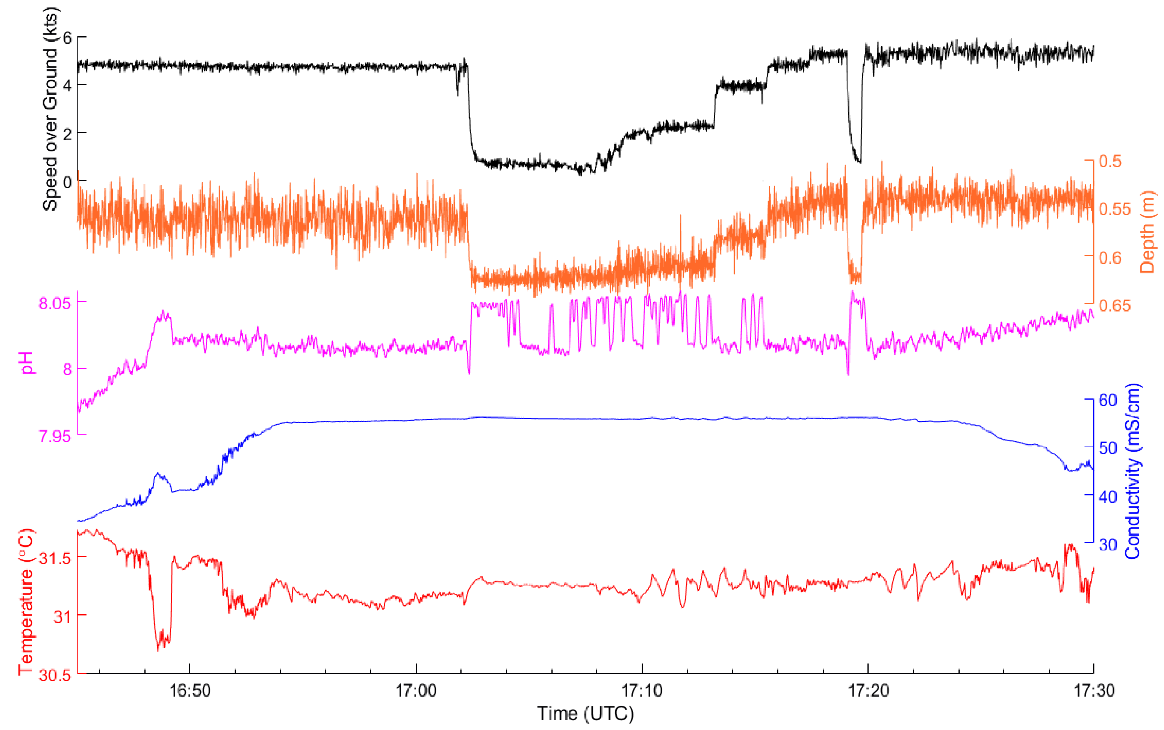
The vehicle can quickly change speeds, although this affects the pH measurements derived from the glass electrode-based Idronaut pH sensor by ~0.035 units (Figure 7). Given that the change in pH is not consistent when speed changes, no offset correction can be applied, and therefore represents an uncertainty, although this uncertainty is much lower than the natural variability identified. Some of this change in pH could be attributed to changes in the sensor depth if there is a vertical structure in the pH profile. When the vehicle is moving, the bow lifts out of the water, raising the sensors. This corresponds to a ~10 cm change in sensor depth when changing from stationary to moving at 5 kts (Figure 7). However, pH values fluctuated during the period of slow speed when sensor depth was constant, suggesting that this may not be the full reason and that further experimentation is necessary.

Vehicle movement can affect fluid dynamics, such as causing turbulent mixing, increased vertical mixing, or the trapping of bubbles when the vehicle speed changes, which may impact the sensor function. At speeds greater than 4 kts, pH readings were more stable, which is likely attributable to associated fluid hydrodynamics; for example, higher speeds may facilitate a steadier flow of water over the sensor with less potential for trapping of bubbles. Further work is required to better constrain the relationship between vehicle speed and sensor function for this type of pH sensor, such as speed tests in a more homogeneous environment with increased bottle sampling for pH analysis. There may additionally be an effect of speed of water flow over the sensor, for which experiments in a laboratory with a pump and water of known pH may be able to identify whether speed of water flow has an impact.

From our field experiments, we conclude that to ensure consistent depth and sensor performance, the vehicle should be set at a consistent speed. For consistency between data collected with the CW4, in terms of both sensor depth and sensor stability, we recommend only using data collected within a narrow range of speeds. We determined 4–5.5 kts yielded the most stable pH measurements. Finally the effect of speed appears to be an issue with the glass electrode pH sensor and not with the conductivity and temperature sensor; therefore, a different pH sensor such as a SeaFET (Sea-Bird Scientific, Bellevue, WA, USA) or a lab-on-chip sensor [40] may yield more stable and accurate results. This, we believe, reinforces the need for validation of all parameters across the full range of relevant operating conditions prior to a deployment of an autonomous platform.

3.5. Identifying Factors Controlling Carbonate Chemistry

Carbon cycling in the coastal environment is dynamic [11], reflecting the environmental diversity and associated complexity of the land–ocean interface. High-resolution data are therefore needed to identify fine-scale spatial changes in various parameters to unpick the factors which control coastal ocean acidification. 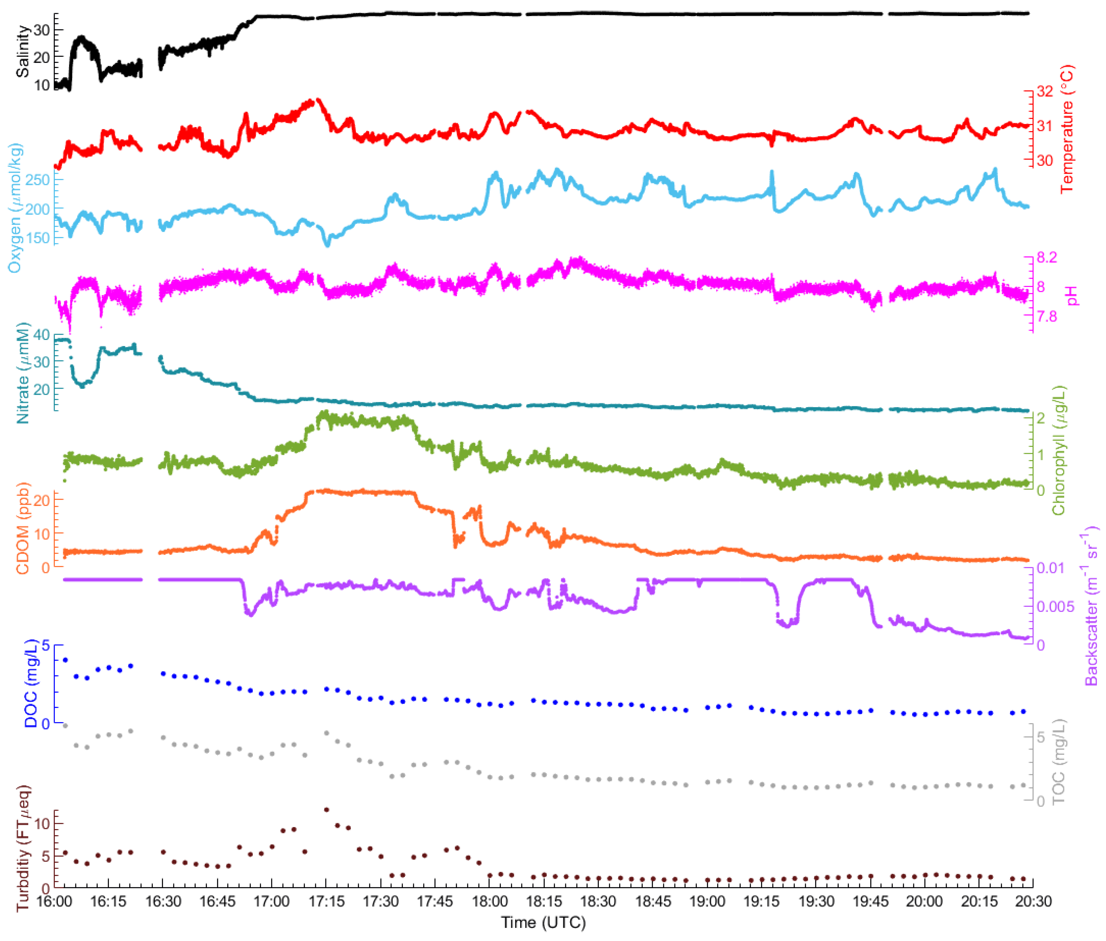Alongside pH and pCO₂, the CW4 collected data for a number of other physical and biogeochemical parameters (Figure 8) including conductivity, temperature, dissolved oxygen, nitrate concentration, DOC, TOC, turbidity, chlorophyll fluorescence, CDOM, and optical backscatter.

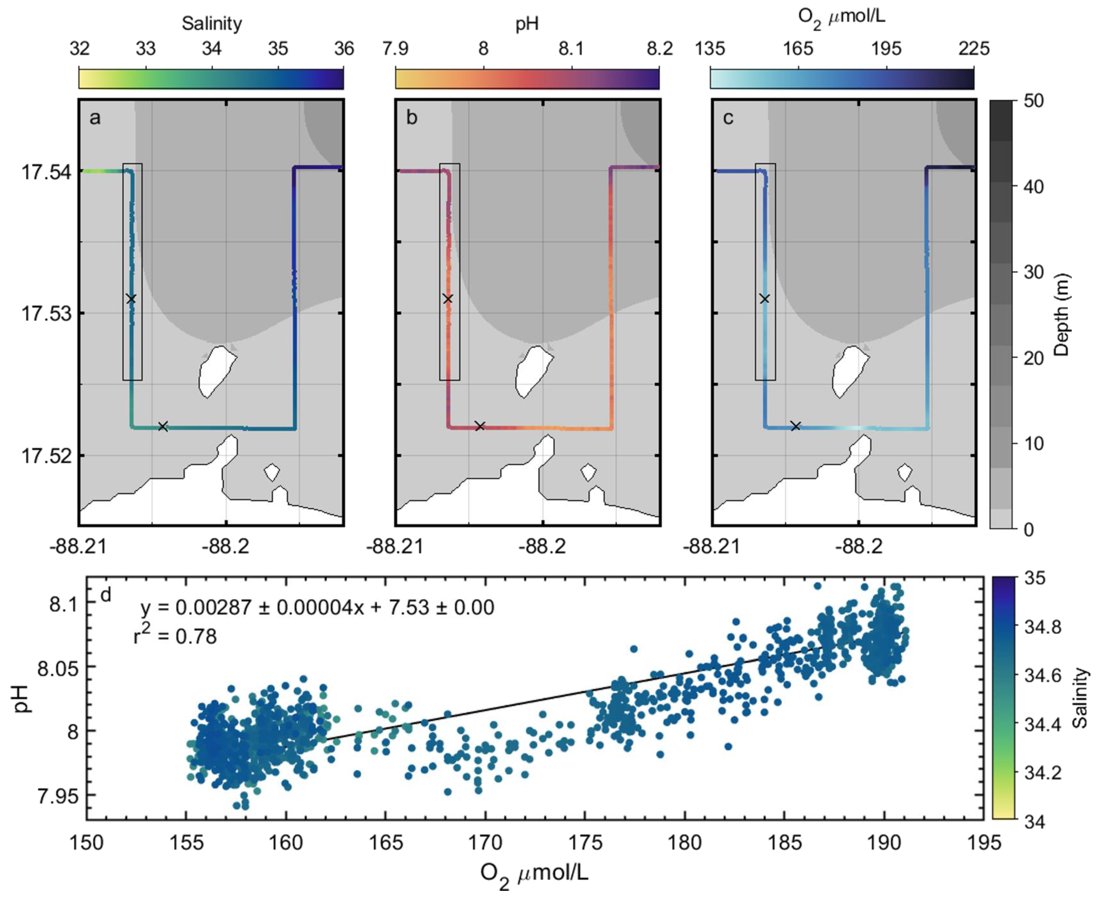
A detailed understanding of biogeochemical processes and controls on the observed spatial pH variability such as ecosystem metabolism and freshwater input can be achieved by integrating the large number of biogeochemical parameters measured concurrently. A good example is shown in Figure 8, where we can begin to see relationships between different parameters, such as increasing chlorophyll, CDOM, TOC, and turbidity at the same time (~17:15), which may be indicative of different process in play. Salinity is a tracer for freshwater input: we identify an inverse relationship between salinity and nitrate, suggesting the Belize River is likely a large source of nitrate to the coastal ocean. We are also able to identify low pH matching low salinity water but while nitrate is low at higher salinity values, we see variation in the pH data. This suggests that while the Belize River is a source of low pH water, there may be other processes at play creating small-scale fluctuations. Co-variation in pH and O₂, for example, could be indicative of the effects of ecosystem metabolism. Since photosynthesis produces O₂ while consuming CO₂, this removal of CO₂ from seawater will allow pH of surrounding water to increase. Figure 9 highlights this co-variation of pH and oxygen over a 1.6 km section of Transect 1 (indicated by black box in the top panels in Figure 9), where pH varied by 0.17, O₂ by 35.9 µmol/L, and salinity by 0.3. The range in pH and O₂ identified greatly exceeds that which would be caused by temperature changes. The temperature range (30.8–31.4 °C) encountered over this section would equate to a 2.34 µmol/L change in O₂ solubility [41] and for every 1 °C, there is a ~0.014 decrease in pH at 1 atm [42]. In this 1.6 km stretch, around 1300 data points were collected for both pH and O₂ by the CW4, whereas only a single discrete sample was taken. Without the autonomous, high-resolution measurements collected by the CW4, a manual sampling regime would fail to capture this small-scale variability and would not be able to fully resolve the carbonate chemistry dynamics in this region.

The capacity to fit a wide range of sensors to CW4, and thus, collect data for different parameters both simultaneously and sequentially, allows the generation of datasets which promote the understanding of processes driving ocean acidification. The CW4′s diesel engine removes the power limitation and restricted payload capacity typically associated with autonomous platforms, thus permitting a greater number of sensors to be mounted in parallel. Sensors can also be easily changed between deployments according to user/science requirements. For example, the CW4 can be fitted with a SideScan sonar or multibeam echo sounder allowing habitat identification, such as coral reefs and seagrass beds. This gives the potential to use a combination of techniques to identify changes in coastal ocean acidification and understand the roles different habitats may be having in mitigating or enhancing ocean acidification. Coral reefs and seagrasses are often in shallow locations, making sampling hazardous and data collection harder, which can lead to data gaps, but they can have a pronounced effect on local carbonate chemistry [14]. Seagrasses are excellent blue carbon stores and consume CO₂ through photosynthesis, which can raise surrounding pH [43], while coral reefs are one of the many habitats sensitive to decreasing pH [44]. CW4 overcomes the hazards associated with data collection in these key habitats, in concert with providing various data streams, which can be integrated to assist in ascribing their relationship to coastal carbonate chemistry.

No single platform will be optimal in all situations; there will always be trade-offs in mission lifetime, payload, power consumption, and measurement frequency [10]. Cameras and passive receivers require only a few watts [45], while instruments like pCO₂ sensors have higher power demands. Having a diesel engine means the payload is not limited by power availability and allows us to cover a much larger area than platforms that use wave and wind for propulsion over a shorter time frame. To cover our four transects in 2019, it would take Wave Glider ~2.5 times as long, based on a speed of 1.5 kts—the average speed of Wave Glider in previous missions [46]. The deployments of CW4 have to be significantly shorter, but the trade-off is high-resolution data for at least 12 different concurrent biogeochemical parameters as well as sampling in shallow waters where most platforms cannot operate. In coastal environments that are more heterogeneous than the open ocean, and where the vehicle can be refuelled more easily, there may be a greater need for higher resolution sampling by sensors and increased sensor load. ASVs evolve to fill a niche which may have been historically under sampled and we think CW4 is ideal for working in shallow coastal seas, which may be home to ecosystems like coral reefs which are potential hazards.

3.6. Recommendations and Best Practices

There is a lack of sustained autonomous observations of carbonate chemistry in coastal regions, despite their great importance for the global carbon cycle [10]. Using autonomous technology, such as the CW4, equipped with a biogeochemical payload, could help to provide sustained coastal ocean observations. This is important in order to track carbon uptake/release and ocean acidification, particularly as there is large natural temporal and spatial variability in the coastal marine environment [47]. Not only is such high spatial and temporal resolution data necessary for understanding evolution of the coastal zone, it is also needed by decision-makers and coastal zone mangers [48]. Autonomous platforms will be a key part of future ocean carbonate systems monitoring [10] and we think that the CW4 will be an important contributor to this.

Here, we present the first demonstration of the ASV CW4 as a tool for ocean acidification monitoring in shallow coastal environments. We have highlighted the need for ASVs in shallow coastal environments and how using sensors mounted upon a surface vehicle facilitates collection of high-resolution data, which can be used to identify sources of low pH, high CO₂ water as well as controls on coastal ocean acidification. Based on our field deployments, in order to improve data collection during future CW4 deployments, we would recommend defining waypoints along lines more regularly and not just on corners to improve track following accuracy. Note that line deviation will be greatest at the corners, so avoid making turns with enough distance from potential hazards. We recommend using pre-planned missions as this allows vehicle speeds to be set and therefore, remain consistent, removing potential effects of vehicle speed on data quality. Best practices suggest the collection of in situ samples over a dynamic range for each variable to better constrain the local dynamics and potentially allow further comparison to other datasets from other regions.

4. Conclusions

To understand the response of coastal environments to natural and anthropogenic forcing factors, like climate change, the coastal system needs to be well characterised and controlling processes understood. However, many of these systems remain unsurveyed on a global scale [48]. The CW4 is a platform that has the capability of being fitted with commercially available sensors and collect high-resolution biogeochemical and oceanographic data that can begin to mitigate this data gap. Equipped with a large biogeochemical sensor payload, we successfully deployed the CW4 in coastal Belize and successfully collected high-resolution carbonate chemistry data, demonstrating its value as a tool to evaluate and resolve the controls of, and to monitor, ocean acidification in a highly dynamic shallow coastal environment. While, on this occasion, we were unable to collect pH and pCO₂ data simultaneously, we have shown separately that both types of sensors can be mounted on the CW4 alongside at least 10 other biogeochemical parameters. Speed was found to impact pH measurements; therefore, operating the vehicle on pre-planned missions at a set speed is recommended to allow comparison across a deployment. Factory calibrated data can be used to evaluate relative changes within the same deployment and map small-scale variability in pH, pCO₂, and ancillary biogeochemical data in a coastal region. Spatial changes can help identify controls on coastal ocean acidification, such as freshwater inputs or ecosystem metabolism. The CW4 is not designed for long endurance surveys, but instead, closer to shore sustained high-resolution mapping surveys (from kilometres to within metres of the coast) that can capture the small spatial scales and dynamics found in shallow coastal regions. In conclusion, we believe that the ability to fit a wide range of commercially available biogeochemical sensors, sample in high-resolution and in shallow waters, follow pre-planned missions, and its remote-controlled capabilities make the CW4 an ideal tool to evaluate ocean acidification and its controls in shallow coastal regions.

References

1. Friedlingstein, P.; Jones, M.W.; O’Sullivan, M.; Andrew, R.M.; Hauck, J.; Peters, G.P.; Peters, W.; Pongratz, J.; Sitch, S.; Le Quéré, C.; et al. Global Carbon Budget 2019. Earth Syst. Sci. Data 2019, 11, 1783–1838. [Google Scholar] [CrossRef] [Green Version]
2. Hoegh-Guildberg, O.E.; Mumby, P.J.; Hooten, A.J.; Steneck, R.S.; Greenfield, P.; Gomez, E.; Harvell, C.D.; Sale, P.F.; Edwards, A.J.; Caldeira, K.; et al. Coral Reefs Under Rapid Climate Change and Ocean Acidification. Science 2007, 318, 1737–1742. [Google Scholar] [CrossRef] [PubMed] [Green Version]
3. Landschützer, P.; Laruelle, G.G.; Roobaert, A.; Regnier, P. A uniform pCO2 climatology combining open and coastal oceans. Earth Syst. Sci. Data 2020, 12, 2537–2553. [Google Scholar] [CrossRef]
4. IPCC. Climate Change 2014: Synthesis Report. Contribution of Working Groups I, II and III to the Fifth Assessment Report of the Intergovernmental Panel on Climate Change; Core Witing Team, Pachauri, R.K., Meyers, L.A., Eds.; IPCC: Geneva, Switzerland, 2014; 151p. [CrossRef] [Green Version]
5. Wallace, R.B.; Baumann, H.; Grear, J.S.; Aller, R.C.; Gobler, C.J. Coastal ocean acidification: The other eutrophication problem. Estuar. Coast. Shelf Sci. 2014, 148, 1–13. [Google Scholar] [CrossRef]
6. Duarte, C.M.; Hendriks, I.E.; Moore, T.S.; Olsen, Y.S.; Steckbauer, A.; Ramajo, L.; Carstensen, J.; Trotter, J.A.; McCulloch, M. Is Ocean Acidification an Open-Ocean Syndrome? Understanding Anthropogenic Impacts on Seawater pH. Estuar. Coast. 2013, 36, 221–236. [Google Scholar] [CrossRef] [Green Version]
7. Cai, W.-J. Estuarine and Coastal Ocean Carbon Paradox: CO2 Sinks or Sites of Terrestrial Carbon Incineration? Annu. Rev. Mar. Sci. 2011, 3, 123–145. [Google Scholar] [CrossRef] [Green Version]
8. Gupta, G.V.M.; Sarma, V.V.S.S.; Robin, R.S.; Raman, A.V.; Jai Kumar, M.; Rakesh, M.; Subramanian, B.R. Influence of net ecosystem metabolism in transferring riverine organic carbon to atmospheric CO2 in a tropical coastal lagoon (Chilka Lake, India). Biogeochemistry 2008, 87, 265–285. [Google Scholar] [CrossRef]
9. Melzner, F.; Thomsen, J.; Koeve, W.; Oschlies, A.; Gutowska, M.A.; Bange, H.W.; Hansen, H.P.; Körtzinger, A. Future ocean acidification will be amplified by hypoxia in coastal habitats. Mar. Biol. 2013, 160, 1875–1888. [Google Scholar] [CrossRef]
10. Bushinsky, S.M.; Takeshita, Y.; Williams, N.L. Observing Changes in Ocean Carbonate Chemistry: Our Autonomous Future. Curr. Clim. Chang. Rep. 2019, 5, 207–220. [Google Scholar] [CrossRef] [Green Version]
11. Nicholson, D.P.; Michel, A.P.M.; Wankel, S.D.; Manganini, K.; Sugrue, R.A.; Sandwith, Z.O.; Monk, S.A. Rapid Mapping of Dissolved Methane and Carbon Dioxide in Coastal Ecosystems Using the ChemYak Autonomous Surface Vehicle. Environ. Sci. Technol. 2018, 52, 13314–13324. [Google Scholar] [CrossRef]
12. Hendriks, I.E.; Duarte, C.M.; Olsen, Y.S.; Steckbauer, A.; Ramajo, L.; Moore, T.S.; Trotter, J.A.; McCulloch, M. Biological mechanisms supporting adaptation to ocean acidification in coastal ecosystems. Estuar. Coast. Shelf Sci. 2015, 152, A1–A8. [Google Scholar] [CrossRef] [Green Version]
13. Gattuso, J.-P.; Frankignoulle, M.; Wollast, R. Carbon and Carbonate Metabolism in Coastal Aquatic Ecosystems. Annu. Rev. Ecol. Syst. 1998, 29, 405–434. [Google Scholar] [CrossRef] [Green Version]
14. Gutiérrez, J.L.; Jones, C.G.; Byers, J.E.; Arkema, K.K.; Berkenbusch, K.; Commito, A.; Duarte, C.M.; Hacker, S.D.; Lambrinos, J.G.; Hendriks, I.E.; et al. Physical Ecosystem Engineers and the Functioning of Estuaries and Coasts. In Treatise on Estuarine and Coastal Science; Wolanksi, E., McLusky, D.S., Eds.; Academic Press Elsevier Inc.: Amsterdam, The Netherlands, 2012; Volume 7, pp. 53–81. ISBN 9780080878850. [Google Scholar]
15. Alves, J.; Oliveira, P.; Oliveira, R.; Pascoal, A.; Rufino, M.; Sebastiao, L.; Silvestre, C. Vehicle and Mission Control of the DELFIM Autonomous Surface Craft I. In Proceedings of the 14th Mediterranean Conference on Control and Automation, Ancona, Italy, 28–30 June 2006; pp. 1–6. [Google Scholar]
16. Saba, G.K.; Wright-Fairbanks, E.; Chen, B.; Cai, W.J.; Barnard, A.H.; Jones, C.P.; Branham, C.W.; Wang, K.; Miles, T. The Development and Validation of a Profiling Glider Deep ISFET-Based pH Sensor for High Resolution Observations of Coastal and Ocean Acidification. Front. Mar. Sci. 2019, 6, 1–17. [Google Scholar] [CrossRef]
17. Johnson, K.S.; Jannasch, H.W.; Coletti, L.J.; Elrod, V.A.; Martz, T.R.; Takeshita, Y.; Carlson, R.J.; Connery, J.G. Deep-Sea DuraFET: A Pressure Tolerant pH Sensor Designed for Global Sensor Networks. Anal. Chem. 2016, 88, 3249–3256. [Google Scholar] [CrossRef] [PubMed]
18. Liu, Z.; Zhang, Y.; Yu, X.; Yuan, C. Unmanned surface vehicles: An overview of developments and challenges. Annu. Rev. Control 2016, 41, 71–93. [Google Scholar] [CrossRef]
19. Karapetyan, N.; Braude, A.; Moulton, J.; Burstein, J.A.; White, S.; O’Kane, J.M.; Rekleitis, I. Riverine Coverage with an Autonomous Surface Vehicle over Known Environments. IEEE Int. Conf. Intell. Robot. Syst. 2019, 3098–3104. [Google Scholar] [CrossRef] [Green Version]
20. Klinck, H.; Fregosi, S.; Matsumoto, H.; Turpin, A.; Mellinger, D.K.; Erofeev, A.; Barth, J.A.; Shearman, R.K.; Jafarmadar, K.; Stelzer, R. Mobile Autonomous Platforms for Passive-Acoustic Monitoring of High-Frequency Cetaceans. In Robotic Sailing 2015: Proceedings of the 8th International Robotic Sailing Conference; Friebe, A., Haug, F., Eds.; Springer: Mariehamn, Finland, 2015; ISBN 9783319233352. [Google Scholar]
21. Pagniello, C.M.L.S.; Cimino, M.A.; Terrill, E. Mapping fish chorus distributions in southern california using an autonomous wave glider. Front. Mar. Sci. 2019, 6, 1–9. [Google Scholar] [CrossRef] [Green Version]
22. Mordy, C.W.; Cokelet, E.D.; De Robertis, A.; Jenkins, R.; Kuhn, C.E.; Lawrence-Slavas, N.; Berchok, C.L.; Crance, J.L.; Sterling, J.T.; Cross, J.N.; et al. Advances in ecosystem research: Saildrone surveys of oceanography, fish and marine mammals in the Bering Sea. Oceanography 2017, 30, 113–115. [Google Scholar] [CrossRef]
23. Nash, J.D.; Marion, J.; McComb, N.; Nahorniak, J.S.; Jackson, R.H.; Perren, C.; Winters, D.; Pickering, A.; Bruslind, J.; Yong, O.L.; et al. Autonomous CTD profiling from the robotic oceanographic surface sampler. Oceanography 2017, 30, 110–112. [Google Scholar] [CrossRef] [Green Version]
24. Desa, E.; Maurya, P.K.; Pereira, A.; Pascoal, A.M.; Prabhudesai, R.G.; Mascarenhas, A.; Desa, E.; Madhan, R.; Matondkar, S.G.P.; Navelkar, G.; et al. A small autonomous surface vehicle for ocean color remote sensing. IEEE J. Ocean. Eng. 2007, 32, 353–364. [Google Scholar] [CrossRef]
25. Mackinnon, J.A.; Nash, J.D.; Alford, M.H.; Lucas, A.J.; Mickett, J.B.; Shroyer, E.L.; Waterhouse, A.F.; Tandon, A.; Sengupta, D.; Mahadevan, A.; et al. A tale of two spicy seas. Oceanography 2016, 29, 51–61. [Google Scholar] [CrossRef] [Green Version]
26. Mullison, J.; Symonds, D.; Trenaman, N. ADCP Data Collected from a Liquid Robotics Wave Glider®. In Proceedings of the 2011 IEEE/OES/CWTM 10th Current, Waves and Turbulence Measurements (CWTM), Monterey, CA, USA, 20–23 March 2011; IEEE: Monterey, CA, USA, 2011; pp. 266–272. [Google Scholar] [CrossRef]
27. Monteiro, P.M.S.; Gregor, L.; Lévy, M.; Maenner, S.; Sabine, C.L.; Swart, S. Intraseasonal variability linked to sampling alias in air-sea CO2 fluxes in the Southern Ocean. Geophys. Res. Lett. 2015, 42, 8507–8514. [Google Scholar] [CrossRef] [Green Version]
28. Chavez, F.P.; Sevadjian, J.; Wahl, C.; Friederich, J.; Friederich, G.E. Measurements of pCO2 and pH from an autonomous surface vehicle in a coastal upwelling system. Deep. Res. Part II Top. Stud. Oceanogr. 2018, 151, 137–146. [Google Scholar] [CrossRef]
29. Sabine, C.; Sutton, A.; McCabe, K.; Lawrence-Slavas, N.; Alin, S.; Feely, R.; Jenkins, R.; Maenner, S.; Meinig, C.; Thomas, J.; et al. Evaluation of a new carbon dioxide system for autonomous surface vehicles. J. Atmos. Ocean. Technol. 2020, 37, 1305–1317. [Google Scholar] [CrossRef]
30. Dickson, A.G.; Sabine, C.L.; Christian, J.R. Guide to Best Practices for Ocean CO2 Measurements; PICES Special Publication: Sidney, BC, Canada, 2007; Volume 3, ISBN 1-897176-07-4.
31. Fassbender, A.J.; Sabine, C.L.; Lawrence-Slavas, N.; De Carlo, E.H.; Meinig, C.; Maenner Jones, S. Robust sensor for extended autonomous measurements of surface ocean dissolved inorganic carbon. Environ. Sci. Technol. 2015, 49, 3628–3635. [Google Scholar] [CrossRef]
32. Briggs, E.M.; Sandoval, S.; Erten, A.; Takeshita, Y.; Kummel, A.C.; Martz, T.R. Solid State Sensor for Simultaneous Measurement of Total Alkalinity and pH of Seawater. ACS Sens. 2017, 2, 1302–1309. [Google Scholar] [CrossRef]
33. Ziegwied, A. Containerized Autonomous Marine Environmental Laboratory—Enhancing Coastal Resiliency with New Technologies. In Proceedings of the OCEANS 2018 MTS/IEEE Charleston, Charleston, SC, USA, 22–25 October 2018; IEEE: Charleston, SC, USA, 2018; pp. 1–5. [Google Scholar]
34. L3Harris C-Worker 4 Autonmous Surface Vehicle User Handbook; 2018; pp. 10–23.
35. Cherrington, E.A.; Ek, E.; Cho, P.; Howell, B.F.; Hernandez, B.E.; Anderson, E.R.; Flores, A.I.; Garcia, B.C.; Sempris, E.; Irwin, D.E. Forest Cover and Deforestation in Belize: 2010–2012. Tech. Rep. 2012. [Google Scholar] [CrossRef]
36. Holley, S.E.; Hydes, D.J. Procedures for the Determination of Dissolved Oxygen in Seawater; James Rennell Centre for Ocean Circulation: Southampton, UK, 1995. [Google Scholar]
37. Karapetyan, N.; Moulton, J.; Rekleitis, I. Dynamic Autonomous Surface Vehicle Control and Applications in Environmental Monitoring. In Proceedings of the OCEANS 2019 MTS/IEEE Seattle, Seattle, WA, USA, 27–31 October 2019. [Google Scholar]
38. Meteored Weather Belize City—Historical Data. Available online: https://www.yourweather.co.uk/weather_Belize+City-Central+America-Belize-Belize+City-MZBZ-1-12275.html?d=historical (accessed on 1 October 2020).
39. Blackford, J.C. Predicting the impacts of ocean acidification: Challenges from an ecosystem perspective. J. Mar. Syst. 2010, 81, 12–18. [Google Scholar] [CrossRef]
40. Rérolle, V.M.C.; Floquet, C.F.A.; Harris, A.J.K.; Mowlem, M.C.; Bellerby, R.R.G.J.; Achterberg, E.P. Development of a colorimetric microfluidic pH sensor for autonomous seawater measurements. Anal. Chim. Acta 2013, 786, 124–131. [Google Scholar] [CrossRef]
41. EIFAC. Report of the Working Group on Terminology, Format and Units of Measurement as Related to Flow-Through and Recirculation System; European Inland Fisheries Advisory Commission: Rome, Italy, 1986.
42. Gieskes, J.M. Effect of temperature on the pH of seawater. Limnol. Oceanogr. 1969, 14, 679–685. [Google Scholar] [CrossRef]
43. Hendriks, I.E.; Olsen, Y.S.; Ramajo, L.; Basso, L.; Steckbauer, A.; Moore, T.S.; Howard, J.; Duarte, C.M. Photosynthetic activity buffers ocean acidification in seagrass meadows. Biogeosciences 2014, 11, 333–346. [Google Scholar] [CrossRef] [Green Version]
44. Jokiel, P.L.; Rodgers, K.S.; Kuffner, I.B.; Andersson, A.J.; Cox, E.; MacKenzie, F.T. Ocean acidification and calcifying reef organisms: A mesocosm investigation. Coral Reefs 2008, 27, 473–483. [Google Scholar] [CrossRef]
45. Hine, R.; Willcox, S.; Hine, G.; Richardson, T. The Wave Glider: A Wave-Powered Autonomous Marine Vehicle. In Proceedings of the Marine Technology for Our Future: Global and Local Challenges, OCEANS, Biloxi, MS, USA, 26–29 October 2009. [Google Scholar]
46. Willcox, S.; Meinig, C.; Sabine, C.L.; Lawrence-Slavas, N.; Richardson, T.; Hine, R.; Manley, J. An Autonomous Mobile Platform for Underway Surface Carbon Measurements in Open-Ocean and Coastal Waters. In Proceedings of the Marine Technology for Our Future: Global and Local Challenges, OCEANS, Biloxi, MS, USA, 26–29 October 2009; pp. 2–9. [Google Scholar]
47. Sutton, A.J.; Sabine, C.L.; Maenner-Jones, S.; Lawrence-Slavas, N.; Meinig, C.; Feely, R.A.; Mathis, J.T.; Musielewicz, S.; Bott, R.; McLain, P.D.; et al. A high-frequency atmospheric and seawater pCO2 data set from 14 open-ocean sites using a moored autonomous systems. Earth Syst. Sci. Data 2014, 6, 353–366. [Google Scholar] [CrossRef] [Green Version]
48. Benveniste, J.; Cazenave, A.; Vignudelli, S.; Fenoglio-Marc, L.; Shah, R.; Almar, R.; Andersen, O.; Birol, F.; Bonnefond, P.; Bouffard, J.; et al. Requirements for a coastal hazards observing system. Front. Mar. Sci. 2019, 6. [Google Scholar] [CrossRef] [Green Version]
Figure 1. Isometric, front and back view of the CW4 (adapted from L3 Harris C Worker 4 Autonomous Surface Vehicle Use Manual [34]).
Jmse 08 00939 g001
Figure 2. (a) Location of the sensor payload on CW4, which is lowered from the hull of the boat and connected to the on board computers (from [34]). Operation can be via remote desktop into these computers. (b) Bottom view of the CW4, highlighting the location of the payload. The payload is retracted into the hull during transportation and for protection when not in use, as pictured. (c) Detailed view of the scientific sensors mounted on a metal plate. Pictured sensors are listed in Table 1.
Jmse 08 00939 g002
Figure 3. Location of the study site in coastal Belize with the CW4 tracks (black lines) and discrete water sampling points (pink triangles). (a) Deployment in November 2018 showing 3 transects, with the north–south transects conducted along the Belize Barrier and around Belize City. (b) Deployment in October 2019 with 4 transects, showing shorter range, but increased spatial variability characterisation.
Jmse 08 00939 g003
Figure 4. Testing of CW4 track following ability and line holding along Transect 1. Zoomed in section in (b,c) is shown in (a) by yellow box. The black line is planned transect marked with waypoints, which creates the lines, and the overlaid pink dashed line is track CW4 completed.
Jmse 08 00939 g004
Figure 5. (a) Modes of operation of the CW4: remotely operated (red line) in the Belize River due the shallow nature of the river mouth and on a pre-planned mission when water depth increased (yellow dotted line). (b) The corresponding speeds for the two operating modes shown in panel (a).
Jmse 08 00939 g005
Figure 6. Carbonate chemistry parameters relevant to ocean acidification collected by the CW4 over two field seasons. (a) pCO2 measurements in 2018 around Belize City showing sensor saturated (>1000 μatm) in the river mouth, (b) pH measurements in Transect 1 in October 2019. Both panels show factory calibrated data. Data shown only for vehicle speeds between 4.5 and 5.5 kts.
Jmse 08 00939 g006
Figure 7. Effect of speed (black) of CW4 on depth (orange), pH (pink), conductivity (blue), and temperature (red). Times are in UTC (+6 h from Belize). Data were collected on Transect 4 on 20 October 2019, are factory calibrated, and smoothed with a moving median of 11 data points.
Jmse 08 00939 g007
Figure 8. Biogeochemical parameters collected concurrently with pH to evaluate controls on ocean acidification. Different panels show an example 4.5 h window of the different parameters: Salinity (black), Temperature (red), Dissolved Oxygen (DO, light blue), pH (pink), Nitrate (teal), chlorophyll concentration (green), coloured dissolved organic matter (CDOM, orange), optical backscatter (purple), dissolved organic carbon (DOC, dark blue), total organic carbon (TOC, grey), and Turbidity (brown). All data have been factory calibrated. Further corrections have been applied to DO (corrected for salinity, temperature, and pressure using CTD data), and pH (corrected for temperature). Salinity, Temperature, DO, pH, Nitrate, Chlorophyll, CDOM, Backscatter, and pH data have all been smoothed with an 11-pt moving median. Further details on the sensors measuring these parameters can be found in Table 1.
Jmse 08 00939 g008
Figure 9. High-resolution sensor data capture small-scale spatial variability in three different parameters in a zoomed in section from Transect 1. (a) Salinity (b) pH, and (c) Dissolved Oxygen. Discrete water sample locations are marked on with an X, rectangle shows 1.6 km stretch where we see changes in pH and O2 but not salinity. (d) Correlation between O2, pH, and salinity from within black box in the top panels.
Jmse 08 00939 g009