Abstract
The Variable Buoyancy System (VBS) is a critical device in the operation of underwater gliders that should be properly sized to achieve the required vehicle propulsion; safety within the operating range; and adequate efficiency at the nominal depth rating. The VBS budget volume depends mainly on the glider hydrodynamics and the main operating states of the vehicle. A method is proposed with analytical equations to analyze the performance of underwater gliders and to estimate the resultant velocities of the vehicle as a function of the buoyancy change and the glider angle. The method is validated to analyze the glider performance of underwater gliders and is essential to get the main design requirement for the propulsion system: the VBS budget volume. The paper presents the application of the method to obtain the VBS sizing for an academic glider; a comparison with the historical hydrodynamic data of the Slocum glider; the results of the glider performance study; and the development of the characteristic charts necessary to evaluate the performance of the vehicle and its flight parameters.
1. Introduction
Oceanography requires the use of a wide variety of instruments, tools, and platforms to study the planet’s water resources. Unmanned underwater vehicles (UUVs), which are piloted with specialized human resources, support and perform special oceanographic operations. In the category of UUV, underwater gliders are autonomous underwater vehicles (AUV) that perform water column sampling for long periods of time and long range transects; gliding in the water at low speed and communicating with the pilot in the surface via satellite to evaluate their performance and to adjust the instructions for the next operation cycle [1].
1.1. Background
Considered the natural evolution of float technology, which are oceanographic devices used for the study of ocean circulation and sampling of water columns [2,3,4,5,6], underwater gliders had an accelerated technological maturation in the 1990s through the program “autonomous oceanographic sampling networks” (AOSN) [7]. In 2001, the development results of the vehicles that are known today as legacy gliders were presented. Slocum, Spray, and Seaglider were developed simultaneously by the Webb Research Corporation (WRC), the Scripps Institute of Oceanography, and the Applied Physics Laboratory (APL) of the University of Washington, respectively [8,9,10,11,12]. Today, the commercial vehicles Slocum and Seaglider are the most popular in the ocean engineering community [13,14].
Jenkins et al. [15] presented the technical report with the results of the development of legacy gliders of the AOSN program; the base theory of the underwater gliders operation [16]. In the report, they describe some of the concepts used for the development of gliders, one of the most important being the concept of specific energy consumption. This concept evaluates the energy balance of the vehicle in a steady state, showing the characteristic charts of the estimated performance of some glider models with respect to the capacity of their propulsion system, called glider polar charts. The charts were obtained as a result of CFD (computational fluid dynamics) analysis tools and mathematical models from the company Vehicle Control Technology, Inc. (VCT) [17,18,19].
The legacy gliders’ main feature is the low energy propulsion engine called the Variable Buoyancy System (VBS), which modifies the net buoyancy of the vehicle to descend and ascend in the water at slow velocity ( m/s). The vehicle glides in the water with steering control systems to change or still the trajectory of the vehicle with the balance of inertial and hydrodynamic forces, generating the characteristic sawtooth movement in the plane [20].
With the development of underwater glider technology, research has been conducted on the dynamics of this type of vehicle to control its main propulsion and steering systems [20,21,22], estimating the hydrodynamic forces of lift and drag in steady state with polynomial regressions as a function of the angle of attack (linear and quadratic equations, respectively). The hydrodynamic polynomial estimations simplify the navigation and flight mathematical models of the vehicle, considering the underwater vehicle as an aerodynamic profile to obtain the polynomial coefficients at small angles of attack.
To obtain the polynomial regressions, it is required to have real or estimated hydrodynamic forces at a defined velocity in the water for small angles of attack (normally between −10° and 10°). Singh et al. [23] presented in 2017 a research paper to validate the use of CFD modeling to estimate the hydrodynamic forces with a variation of the angle of attack between −8° to 8° with steps of 2°. The CFD method was validated by the experimental results of the glider in a towing tank with the same specifications.
In the absence of a defined methodology for the development of VBS for underwater gliders, a preview of this article [24] was presented in 2018 with the first results of the theoretical work on the development of a VBS for an academic glider of 200 msw (meters of salt water) depth rating called Kay Juul 2 (from the Mayan “Row Fish”). The work presented the glider performance charts and the analytical equations based on polynomial coefficients to estimate the velocity of the vehicle in steady state and the VBS budget for the nominal velocity of operation. The polynomial coefficients were obtained by Bustos et al. [25] with CFD modeling based on [22,23] with angles of attack between −15° and 15° with steps of 5°.
The results of [24] show the direct dependence on the hydrodynamic coefficients [25] and the flight angles in the VBS displaced volume, highlighting the importance of the design requirements and the hydrodynamic parameters of the vehicle to estimate the VBS budget. The equations and charts of [24] have been updated for the present research in order to propose a practical method to estimate the VBS budget as a result of the glider performance analysis and the main operation states. One important correction is the variability of the angle of attack as a function of the desired glide slope or glide angle, considered previously as a constant.
Tiwari and Sharma [26] in 2020 presented a methodology to select and analyze VBSs for AUVs through buoyancy control, which emphasizes the importance of defining the design requirements and subsequently selecting the most appropriate type of VBS. These factors are necessary to generate the conceptual design for the computational simulation model and its analysis; the VBS volume is one of the design requirements that need to be defined. The purpose of the present research on underwater gliders is to propose a method to define the VBS volume capacity for its design process, given that “the design process of a VBS system is not known in full, and existing approaches are not scalable” [26].
In 2020, Eichhorn et al. [27] presented the performance analysis of the Slocum glider based on polynomial coefficients to improve its navigation, comparing different historical hydrodynamic models of the legacy vehicle. Their method used the polynomial coefficients to estimate the performance with a variation of the angle of attack.
Another glider performance study was presented in 2020 by Deutsch et al. [28], using semi-empirical equations for each major component of the Slocum vehicle (body, wings, and vertical tail); assuming a constant angle of attack (optimal angle of attack) and increasing the error in the velocity estimations while the glide angle is incremented. The semi-empirical equations are dimensionless lift and drag coefficients for different components and wings that depend on the attack angle, and the Reynolds number.
1.2. Research Contribution
The proposed method in this article presents analytical equations that consider the underwater glider as an asymmetrical profile, as well as presenting a particular solution for symmetrical profiles. The particular solution is validated with the results in [27], simultaneously using polynomial coefficients for the hydrodynamic forces and considering the coefficients in the operating velocities of the vehicle as stable. The main advantages of the proposed method respect to [27] are mentioned as follow:
- The glide angle is an input parameter and main variable. All the output parameters are in function of the desired glide slope of the vehicle, even the flight angles; calculating first the angle of attack and then the pitch angle (controlled by the internal mechanism of the vehicle).
- The VBS sizing process is included in the results of the performance analysis in order to obtain one of the main design requirements for the propulsion system. No approach is reported to define the VBS budget volume for underwater gliders, except the previous work presented in 2018 [24].
- The method considers the entire vehicle to have an asymmetrical profile or to have asymmetrical wings when defining the descent (dive) and ascent (climb) state solutions.
The analytical equations to evaluate the glider performance analysis are presented to obtain the relation between the VBS and the glider performance in different operation points. In the early design states, the performance analysis is important to size the main mechanisms. The detailed design state could be used to estimate the vehicle performance with updated information, such as detailed CFD analysis of the vehicle with sensors and other components that could modify the hydrodynamics.
This paper proposes a practical method to analyze the glider performance, including the VBS sizing process as an output resultant of the analysis process. The main characteristic charts are presented to analyze the effect of the polynomial coefficients in the performance of the vehicle. The discussion about the improvement of resultant velocity with respect to the displaced volume of the VBS, and the effect of the polynomial coefficients is presented. The approach of the proposed method is to consider the VBS sizing as an important design requirement for the propulsion of the vehicle, however, the glider performance analysis could be expanded to obtain the sizing of the other main mechanism (i.e., for the pitch mechanism stroke with the analysis of hydrodynamic torque compensation).
The structure of the paper is as follows. The flow chart of the proposed method to analyze the glider performance and the outputs of the method are shown in Section 2; including the VBS sizing. Section 3 describes the main operation states of the underwater gliders and the principle of operation to define the concept of the VBS budget. In Section 4, the performance analysis of underwater gliders is presented, obtaining the analytical equations needed to evaluate the performance of the vehicle; the estimation of flight and the estimated volume of the VBS. In Section 5, the results and discussion are presented, validating the glider performance analysis equations and obtaining the outputs of the method; calculating the VBS budget for the glider Kay Juul 2, and generating the characteristic charts to evaluate its performance. Finally, Section 6 presents the conclusions about the importance of the glider performance analysis in the VBS sizing.
This research is divided in two papers: the first one that is presented in this paper has the main contribution to propose the general method to obtain the VBS sizing and the glider performance analysis based on polynomial coefficients; the second one is the modeling, development, and efficiency study of the VBS type piston tank for the academic glider Kay Juul 2.
In Table 1, the required variables for the development of this paper are listed.

Table 1.
List of variables used to describe the glider operating states in steady state.
2. Glider Performance Method with VBS Sizing
Figure 1 shows the flow chart of the proposed method to perform the glider performance study to calculate the VBS budget volume for underwater gliders, using the analytical equations presented in the next sections.
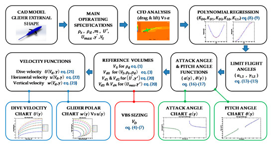
Figure 1.
Chart of the glider performance analysis method focused on VBS sizing.
In the first line of Figure 1, it is observed the process to estimate, by CFD modeling the polynomial coefficients required for the glider performance study [23,25]. The validation process for CFD in a laboratory with a towing tank [23] is preferred but not mandatory. To achieve the estimation of coefficients in nominal operation of the vehicle, it is recommended to perform the CFD analysis with the water density at depth rating , the nominal dive velocity of design , and the variation of the angle of attack to be between −10° to 10°. The use of a higher range of angle of attack for the analysis could result in a deviation of the linear fitting caused by the stall effect at low Reynolds number [29], and subsequently in the estimation of the lift polynomial coefficients.
In the center line of Figure 1, it is observed the main process of the glider performance study. With the hydrodynamic forces estimated with polynomial coefficients, the limit flight angles are calculated: the optimal attack angles and the minimal operating glide angles . With the limit flight angles, the theoretical glide range is defined from [−90°,] for the descent (dive) state and [,90°] for the ascent (climb) state. The output functions for the attack angle and the pitch angle (measured with the internal compass of the vehicle) are obtained as a function of the glide angle.
Then, the reference volume of the VBS as a function of the desired velocity and the glide angle is obtained. With the main specifications defined above, the reference displaced volumes at the main operating states, defined in Section 3, are computed to calculate the VBS budget volume for the propulsion system.
Finally, the velocities of the vehicle as a function of the displaced volume and the glide angle are obtained, generating the charts that estimate the performance of the vehicle at different points of operation. In the third line of Figure 1, the outputs of the proposed method are shown.
3. General Operation States of Underwater Gliders
In the Handbook of Ocean Engineering [16], the underwater gliders are described as a winged vehicle propelled by buoyancy changes, for which the mechanical force of locomotion, necessary to overcome the drag of the vehicle as it moves through a fluid medium, is supplied by gravitational force in the form of net buoyancy (positive or negative). The change in the net buoyancy is generated with the VBS system, which is the main propulsion system of the underwater gliders.
Even though underwater gliders can operate in different modes such as spiraling motion [22] or virtual mooring [30,31,32]. The basic modes are based on their movement in the vertical plane (), generating the characteristic “sawtooth pattern” in each cycle of operation as shown in Figure 2, while sampling the physical and chemical parameters of the water with respect to the operating depth (water column sampling) through the installed scientific sensors and the sampling configuration designated by the glider pilot. The sensors that are most commonly installed in these vehicles are the CT (conductivity-temperature) and the CTD (conductivity-temperature-depth) sensor, with which the operating density of the vehicle is indirectly estimated during the mission.
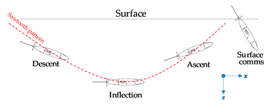
Figure 2.
Sawtooth pattern and main operation states in the underwater glider operation cycle.
In Figure 2, four of the most important operating states of a glider are shown. These states correspond to the different state changes of the VBS and other vehicle subsystems which are used to generate the forward movement at a resultant glide angle.
3.1. Descent and Ascent States
In Figure 3, the schematic diagram of inertial forces (red) and the hydrodynamic reactions (blue) in the descent and ascent state of the glider are shown. In the descent state, the negative net buoyancy causes the vehicle to glide downwards in the water, eventually reaching a stable state at a constant speed through the balance of the hydrodynamic forces and inertial forces. In the ascent state, the positive net buoyancy causes the vehicle to glide upwards, also reaching the steady state. The result in both states is the forward movement of the vehicle with an estimated glide angle (Section 4). In the steady state, the resultant hydrodynamic force is in the opposite direction of the net buoyancy force .
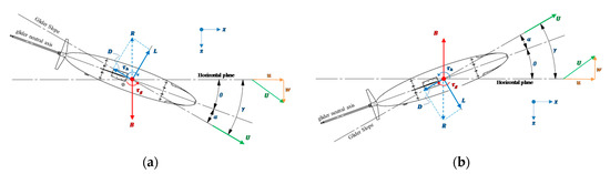
Figure 3.
Underwater glider movement at steady state for: (a) descent state (b) ascent state.
According to Newton’s first law, for the vehicle to be in a steady state at constant speed, the vehicle must be in equilibrium (the sum of forces and moments is equal to zero), therefore the dive velocity will be the result of the balance of the inertial forces and the hydrodynamic reactions.
Considering that the pitch angle is controlled by the unbalance of the internal masses of the glider (the pitch mechanism), the analysis to estimate the flight angles, as a function of the glide angle , is presented in Section 4.
3.2. Inflection State
In Figure 4, the schematic diagram of the vehicle in the inflection state or neutral buoyancy state is shown. This state is the transition between the descent and ascent states, where the VBS increases the buoyancy force to balance the weight of the vehicle, obtaining a net buoyancy force that is equal to zero or neutral buoyancy (), slowing down the vehicle and reducing the hydrodynamic reactions until it reaches the state of rest (). This state is commonly used to obtain the reference point of the VBS () in order to estimate the budget and the velocities of the vehicle, as well as to adjust the flight parameters during the mission. In practice, the underwater gliders are subjected to a process of ballasting before a mission to estimate the point of neutral buoyancy through prediction tools that come with the commercial vehicles.
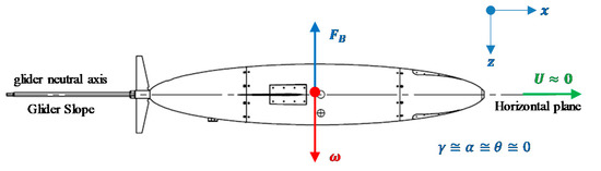
Figure 4.
Schematic diagram of Inflection state of an underwater glider.
In the inflection state, the components that are in contact with the water are subjected to compression by the hydrostatic pressure and, therefore, to a reduction in the displaced volume that needs to be compensated by the VBS system in the operation depth. The volume reduction depends on the mechanics of the materials and the design of each component. On the other hand, the stratification in the ocean can compensate for the decrease of volume given the increment of density of the saltwater with respect to the operation depth [15]. For example, the vehicle Seaglider is designed with a special pressure hull, which compensates itself for the volume reduction by the hydrostatic pressure with the increment of density, generating a buoyancy force similar to that found at the surface, but at 1000 msw depth [11].
The calculation of the volume compensation at the inflection point of the vehicle is outside the scope of this article, however, it is recommended to take it into account as part of the comprehensive study of a glider to be considered in the VBS budget.
Thus, neglecting the compensation of VBS by the compression of the pressure hull, the reference volume for the neutral buoyancy state is defined in Equation (1):
3.3. Surface Comms State
In Figure 5, the schematic diagram of the vehicle in the surface comms state is shown. In this state of the operating process, the vehicle is in the state of rest, floating on the surface with a section protruding out of the water so that it can communicate with the command center via satellite; sending information about the operating cycle, its position and receiving instructions from the pilot to continue with the mission or to wait to be recovered.
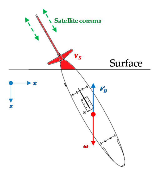
Figure 5.
Schematic diagram of the surface comms state of an underwater glider.
Since a section of the vehicle is out of the water, the volume that was previously submerged no longer provides buoyancy in this state, for which it has to be compensated by the VBS. The compensated buoyancy force can be calculated by Equation (2):
Substituting the value of the reference volume from Equation (1), the required volume to be displaced by the VBS for the surface comms state is obtained as shown in (3):
Therefore, if the density of the fluid and , the mass of the balanced vehicle and the required volume out of the water are known, the volume required to maintain the vehicle in the surface comms state can be calculated from neutral buoyancy to execute satellite communication with the command center.
3.4. VBS Budget
The propulsion system VBS for underwater gliders must have enough volume capability to generate the required speeds in the descent and ascent states, and the required volume to operate in the surface comms state. Therefore, once the main operating states of the vehicle have been described, the operating points of the VBS have to be identified to determine its sizing.
In Figure 6, a general diagram is shown with the different points of volume displacement that the VBS system needs to generate the different operating states. These points are measured with respect to the state of neutral buoyancy or inflection state with the reference volume , generating upward movements for and downward movements for .
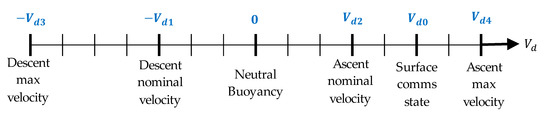
Figure 6.
Basic VBS states for glider operation.
Figure 6 shows two states of descent, two of ascent, the state of neutral buoyancy with the volume reference value , and the surface comms state with a reference volume calculated with Equation (3). As mentioned in Section 3.1, the estimation of the displaced volume for the descent and ascent states, at nominal and max velocity, depends on the analysis of the glider performance of the glider that is described in Section 4.
Obtaining the values of each of the descent and ascent states, the sizing of the VBS system can be estimated by means of Equation (4) or (5) depending on the application case:
Therefore, Equations (4) and (5) consider the size limits of the VBS with the minimum volume capacities to reach the nominal velocities in descent and ascent. However, if the calculation is carried to its limit capacity to perform maximum velocities, the dimensioning of the VBS can be estimated with Equations (6) and (7):
It is not recommended to perform the sizing of the VBS with the limit values of Equations (4) and (5) because in practice it is necessary to have an additional VBS volume budget to overcome low and moderate currents. It is recommended to perform the calculation of the VBS capacities using Equations (6) and (7) in order to have a budget that is more adequate to the vehicle’s operating capacities. For example, in the case of the commercial vehicle Seaglider, it has a budget for its VBS system that allows to overcome average currents of up to 40 cm/s with a maximum volume displacement of = 350 cc with respect to its neutral buoyancy point, moving with vertical speeds of approximately 20 cm/s [33,34].
The calculation of the volumes found in Equations (4) and (5) can be considered as a point of reference to estimate a base volume for considering an operating environment without sea currents or to estimate the energy consumed in a specific mode of operation for deeper analysis.
Section 5 presents the study of the hydrodynamic performance of underwater gliders, which shows that the basic flight parameters of the vehicle and the limit volumes used to size the VBS system can be estimated through analytical relationships and analyzed with glider polar charts.
4. Glider Performance Analysis
This section presents the performance analysis of the underwater gliders in order to obtain the characteristic equations for the estimation of the basic flight parameters and the required sizing of its VBS propulsion system.
Considering the underwater glider as an asymmetrical aerodynamic profile at small angles of attack, the hydrodynamic forces are modeled as follows:
where and are the polynomial coefficients used to estimate the hydrodynamic forces of drag and lift respectively, both dependent on the turbulence regime (), the fluid density and the characteristic area . Considering that the coefficients and are stable in the vehicle’s operating range, they can be considered as a constant for practical purposes of glider performance analysis. As shown in the Figure 7, the drag force is in line with the glider slope line and perpendicular to the lift force. It is observed that the resultant balances the buoyancy force .

Figure 7.
Free body diagram of the underwater glider in descent state.
4.1. Energy Balance and Geometric Analysis
The energy balance of the underwater glider flying at constant velocity with a glide angle is obtained by the power developed by the gravitational force and the power needed to overcome the drag generated by the hydrodynamic response of the vehicle [15,16]. Due to the fact that in the steady state , and the net buoyancy could be defined by Equation (10):
To evaluate the glider performance, the concept of specific energy consumption was used by Jenkins et al. [15,16]. It is desired for the specific energy consumption to be minimal in order to obtain the highest rate between lift and drag in a plane, as is shown in Equation (11):
It can be observed in Figure 7 that to achieve the balance of forces needed for steady state, the hydrodynamic components utilize the glide angle defined in Equation (11).
Substituting the drag and lift forces from (8) and (9) into (11), obtains the specific energy consumption of the glider as a function of the hydrodynamic coefficients and the angle of attack:
To obtain the minimal value of , Equation (12) is derived with respect to the angle of attack (), obtaining the limit values of the angle of attack as follows:
Substituting the solutions from (13) into (12), two specific energy consumption values are obtained, which represent the minimum energy consumption in ascent state and descent state . With the minimum energy consumptions, the next values of the glide angle are obtained:
where and represent the minimum glide angle values for which the balance of hydrodynamic forces with the buoyancy force is valid.
Considering that the glide angle is an input parameter to calculate other flight parameters of the vehicle, the attack angle is obtained by solving Equation (12) as a function of the glider angle as is shown in the solution (16):
where and are the angles of attack functions in ascent state and descent state respectively, considering that there are two limits or discontinuities that are defined by (13).
Thus, the pitch angle will be obtained by subtracting the value of the angle of attack from the glide angle:
4.2. Symmetrical Profile Consideration
If the shape of the glider is close to a symmetrical profile with respect to the middle plane of the vehicle, the wings have a symmetrical profile and are aligned with the glider’s neutral axis; the lift force value in could be neglected (). In the same way, when , the drag curve will tend to be symmetrical, thus the coefficient of the linear parameter could be neglected (). The reduced solutions of Equations (13) and (16) are as follows:
The equations developed in Section 4.1 and Section 4.2 are validated in Section 5 with the research of Eichhorn et al. [27], leading a discussion about the results and the potential of use of the present methodology.
4.3. Glider Polar Chart Equations-Velocity Analysis
According to the principle of Archimedes, the net buoyancy force is defined by , where the reference displaced volume was defined in the Section 3.4 with the main operation states of the vehicle. Substituting the buoyancy expression from (8) into (10), the next equation is obtained to calculate the required displaced volume in function of the hydrodynamics:
If the vehicle’s max velocity during descent and ascent; the hydrodynamic coefficients; the fluid density; and the required glide angle are known, then the reference volume and , as described in Section 3.4, could be obtained, calculating first through (16).
Subtracting the dive velocity from Equation (20), the analytical equation to calculate the resultant velocity as a function of the displaced volume , the fluid density , and the hydrodynamic parameters and the glide angle are as follows:
where the projections of horizontal velocity and vertical velocity are obtained in (22) and (23):
Equations (21)–(23) can generate the characteristic performance charts of underwater gliders; generating contour curves with different values and making sweeps with respect to the glide angle . This in turn calculates the angle of attack that varies with respect to angle . The resultant velocity variation with respect to the glide angle ( vs ) is called the “dive velocity chart”. The “glider polar chart” is the horizontal velocity graph on the abscissa axis and the velocity on the ordinate axis ( vs ). Both charts are obtained in the next section in order to discuss the analysis process based on the proposed method.
5. Results and Discussion
In the analysis of glider performance of Eichhorn et al. [27], the lift and drag forces have been modeled as first and second degree polynomial equations in function of the angle of attack , without considering the coefficient of the independent term for the lift () and the coefficient of the first degree term (), such as the model of a symmetric profile (Section 4.2).
5.1. Limit Flight Angles
To validate the equations, the results of Eichhorn et al. [27], who used the historical data of the hydrodynamic studies with the Slocum gliders, are presented in Table 2. The values obtained by Equations (12)–(15) match with the values obtained by Eicchorn et al. [27], therefore the validation process of the equations is correct and can be used to perform the glider performance analysis.
Table 2.
Validation of energetic and geometric equations.
The hydrodynamic coefficients of the vehicle Kay Jull 2 [25] are included in the Table 2; this vehicle is a winged body of revolution with an ellipsoidal external shape, a fineness ratio of 6.6, and a body length of 2 m. The polynomial coefficients of [25] have been updated to have regressions of between −10° to 10° of the angle of attack to improve the linear function, this was because the lift state presents a stall effect close to the angle of attack of 10° and the previous regression considered a range between −15°to 15°. Both models have been considered in the discussion of the results.
5.2. Comparative Performance Charts
Figure 8 show the variation of the angle of attack for the models listed in Table 2, calculating the attack angle with Equation (16). The negative glide angles represent the vehicle in descent state and the positive angles in ascent state.
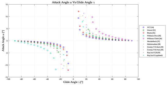
Figure 8.
Attack angle variation chart of the hydrodynamic models.
As a result of the estimation of hydrodynamic parameters from symmetric profiles, the behaviors of the angles of attack at positive and negative glide angles mirror each other, as observed in Figure 8, except for the model of Williams [36] which is defined with coefficients for the dive (descent) and the climb (ascent) states.
It is observed that the curves stop growing at the values of maximum angle of attack and the minimum glide angle obtained in Table 2, representing the limit values of flight angles where the hydrodynamic forces can compensate the buoyancy force in forward movement in steady state, generating a non-operating zone where the equations have no real solution. The angle of attack has an accelerated growth when the glide angle is close to the limit values of operation, so the estimation of the attack angle that corresponds to a flat glide slope becomes relevant for the performance of the vehicle.
In Figure 9, the variation of the pitch angle is shown as a function of the glide angle calculated with Equation (17).
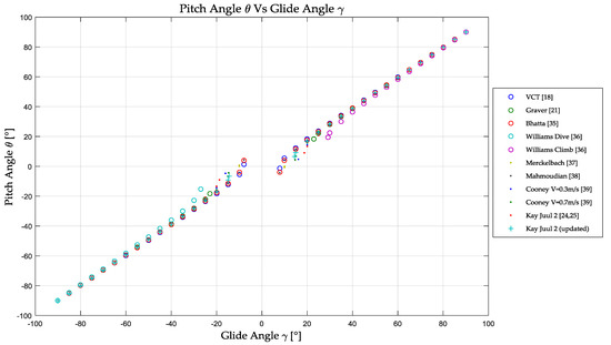
Figure 9.
Pitch angle variation chart of the hydrodynamic models.
It can be observed that for almost all the models analyzed, the value of the pitch angle is approximately equal to the value of the glide angle for values greater than 20°, except for the Williams models [36], which has a minimum glide value of about 28° that causes a considerable deviation around the limit. The Graver model [21] also has a glide angle limit value greater than 20° but its maximum angle of attack is relatively small, and so no significant deviation is observed for it in Figure 9. This means that it is not necessary to have a small glide angle limit to have a small angle of attack.
Figure 8 and Figure 9 also show that when the glider requires a glide angle of 90° (completely vertical movement), the angle of attack will tend to zero for symmetrical profiles, and, theoretically, the vehicle could perform movements or cycles of virtual mooring [30,31]. Perhaps the vehicle could be limited to perform only a certain range of this pitch angle with the internal movement of masses that depend on the design of the internal mechanisms of the glider.
Moreover, the maximum limit of the glide angle should be determined by the ability of the internal mechanism of the vehicle to control the pitch angle, which is out of the scope of the present paper. However, it is important to mention it, so as to improve the present research in the future and to have a more robust method to analyze the performance of underwater gliders.
Considering a displaced volume cc and a density of water of kg/m3, Equation (21) obtains the dive velocity chart that is shown in Figure 10 so that it can be compared to the models listed in Table 2.

Figure 10.
Dive velocity chart of the hydrodynamic models at cc.
It is observed that from about 35° of the glide angle, the velocity that could perform the analyzed models follows an order with respect to the value of the polynomial coefficient . This occurs because the angle of attack and the factor in Equation (21) becomes too small, and the dive velocity is affected mainly by the coefficient.
For glide angles below 35°, where the gliders normally operate, the dive velocity does not always follow the same trajectory and the value of the factor could modify the tendency. For this reason, it is important that throughout the entire operation range, all variables are considered without assumptions, especially the angle of attack.
Calculating the velocity components with Equations (22) and (23) and considering a displaced volume cc, the glider polar chart in Figure 11 is obtained so that it can be compared to the models listed in Table 2.

Figure 11.
Glider polar chart of the hydrodynamic models at cc.
Figure 11 shows a comparative chart of the estimated velocities of the hydrodynamic models under the same displaced volume as the glider polar chart. At the same time, with the information in Figure 10, an important variation in the velocities obtained for the same vehicles is observed. For example, at a 35° glide angle, the Slocum models have a dive velocity increment of 1.77 times in the VCT model [18] with respect to the Conney model [39], and an increment of 1.9 times at 20°. In the case of the vehicle Kay Juul 2, an increment of 1.12 times with respect to the original coefficients [25] is obtained at 35°, and an increment of 1.24 times at 20°, with a correction in the regression range.
The parameter described by Jenkins et al. [15,16] of minimal specific energy consumption has a direct relation with the minimal glide angles , that is the minimal operational flight angle to have the maximal traveled distance per cycle. The operational velocities obtained depend mainly on the drag coefficient at a zero angle of attack . Thus, both parameters have to be considered to improve the performance of the vehicle.
To have the maximum horizontal velocity, the value of the glide angle can be obtained by solving Equation (24), considering a symmetrical profile () and neglecting the factor for small angles of attack. Then, considering the terms inside the root as a constant, the optimal glide angle is obtained as follows:
Jenkins et al. [15,16] mentioned that the maximum along-coarse speed (horizontal speed) in still water is always obtained at a 35° glide angle, regardless of the vehicle shape or other hydrodynamic property. Eichhorn et al. [27] obtained the same result, optimizing their function of the horizontal velocity by considering as a constant for small angles of attack.
Exceptions are observed in Figure 11 in the Graver [21] and the Williams models [36]. The maximum horizontal velocities are obtained about 40° and they have the limit glide angles close to 35°. If the higher values of the limit glide angles could be the cause of the exception, it is recommended to verify the results and output charts to validate the estimations of the glider performance.
One potential application of the proposed method of asymmetrical profiles is an underwater glider concept with asymmetrical wings. Its conceptual design was presented in 2019 in the 8th EGO (Everyone’s Gliding Observatories) meeting [40]; however, the hydrodynamic parameters of the vehicle have not been published, although it could be interesting to evaluate in detail.
5.3. Kay Juul 2-VBS Sizing
Considering that the glider Kay Juul 2 has a weight of 90 kg, the density of the operation is 1024 kg/m3 in the surface and 1026 kg/m3 in the depth rating; the nominal glide angle is 35°; the maximum dive velocity in descent and ascent state of 50 cm/s; the estimated volume outside the water in surface comms state is 400 cc; with a nominal velocity of 35 cm/s. The computed reference volumes and the VBS budget are shown in Table 3.
Table 3.
Reference volume computed for the glider Kay Juul 2.
The reference volumes and were computed with Equation (20) at max velocity and nominal velocity, respectively. The volume was computed with Equation (1) and the and were obtained by the mirror property of the symmetrical profiles ( and ).
According to Section 3.4, the total volume is obtained through the reference volumes. By substituting the values in Equation (7), the required VBS budget of the academic glider Kay Juul 2 can be obtained for the values presented in [24,25] as well as the updated polynomial coefficients.
The difference in VBS budgets is 99.24 cc, representing a deviation of 9.85%, by simply updating the polynomial coefficients with the correct glide angle range, obtaining the same results of the CFD analysis [24]. In the next subsection, the comparative performance charts of the two models at different displaced volumes is presented.
5.4. Kay Juul 2-Performance Charts
Obtaining the reference volumes of the vehicle, in Figure 12 and Figure 13, the glider polar chart and the dive velocity chart are shown for the academic glider Kay Juul 2 with the updated polynomial coefficients, and in the Figure 13, the dive velocity chart, generating curves each 100 cc of volume capability, beginning with 100 cc and finishing with the max displaced volume from the neutral buoyancy state, .
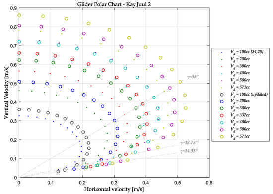
Figure 12.
Glider polar chart—Kay Juul 2.

Figure 13.
Dive velocity chart—Kay Juul 2.
In Figure 12 and Figure 13, two different marks are observed: The point marks represent the results with the hydrodynamic coefficients presented in [24,25] and the circle marks represent the values for the updated coefficients.
It is observed that particularly in this case, with the adjustment in the polynomial regression for the hydrodynamic coefficients, the model has been improved. The minimal glide angle changed from 18.73° to 14.33°, representing an improvement of 23.5% with respect to the previous model. The required volumes to perform an output velocity of 35 cm/s and 50 cm/s at 35° of glide angle, have a reduction of 22.74% with respect to the model without adjustment.
As is commented in the analysis of Section 5.2, the improvement of the model updated for Kay Juul 2 has two main directions described as follows:
- The value of in the updated model was decreased, obtaining an increment of the velocity at the same displaced volume with respect to the previous model. This means that to improve the velocity performance with respect to the displaced volume, it is necessary to reduce the resultant drag force at the zero angle of the glide angle. That could be done, for example: using a lower fineness ratio (rate between the external diameter and the length of the vehicle); reduction in the superficial roughness of the external shape; reduction of the dimensions of the vehicle; other techniques to reduce the basic drag.
- The limit glide angle was reduced. That means that the optimal lift and drag ratio was increased and the specific energy of consumption was reduced. If the reduction in the specific energy consumption is not a determinant to improve the velocity performance of the vehicle, it is observed in the comparative charts of the Section 5.2 that the curves are more stable. In combination with the reduction of the angle of attack, the velocity function in Equation (21) and the displaced volume in Equation (20) are improved because the factor is reduced too, obtaining more velocity with respect to the displaced volume of the VBS.
Comparing the estimated performance of the glider Kay Juul 2 with respect to the models of the Slocum [27], the performance of the functions of flight angles is acceptable and the velocity curves are stable. The limit of the angles of attack is the second lower value of the analyzed models and the limit of the glide angle is on the average zone. The dimensions of the vehicle Kay Juul 2 are bigger than the Slocum dimension; therefore, the polynomial coefficients of the vehicle are also bigger, resulting in a lower resultant velocity at the same displaced volume as the Slocum models.
6. Conclusions
In this paper, the performance of underwater gliders is analyzed and discussed in detail in order to estimate the adequate volume capacity of the VBS as an important design parameter. The proposed method is described and the analytical equations are obtained to estimate the output functions. The outputs of the method to estimate the flight angles, and the resultant velocities are obtained as a function of the glide angle. The characteristic charts of the method are obtained to evaluate, and to compare the performance of the vehicle with respect to other designs. The value of the angle of attack in the operational glide angles () is discussed at detail to improve the estimation of the output functions in the method; including the displaced volume by the VBS. It is recommended that throughout the entire operation range of the vehicle, all variables are considered without assumptions, especially the angle of attack to improve the estimation of all the values.
The method was applied to compare glider performance of the Slocum and the Kay Juul 2 models, obtaining the characteristic charts to discuss the relation between the hydrodynamic coefficients, the limit flight angles and the output functions of the method.
The VBS sizing, considered an output of the method, was applied to calculate de VBS budget of the glider Kay Juul 2, generating at the same time the glider polar chart and the dive velocity chart to analyze the performance of the vehicle at the limits of the displaced volume of the VBS, verifying that the main operating specifications have been satisfied.
This research is part of the results of the development process of an academic glider called Kay Juul 2 (from the Maya “Row Fish”) in order to assimilate the underwater glider technology.
Author Contributions
Conceptualization—J.P.O.-M. and T.S.-J.; methodology—J.P.O.-M.; software—N.A.R.-O.; validation—J.P.O.-M. and T.S.-J.; formal analysis—J.P.O.-M.; investigation—J.P.O.-M. and N.A.R.-O.; resources—T.S.-J.; data curation—J.P.O.-M. and N.A.R.-O.; writing-original draft preparation—J.P.O.-M.; writing-review and editing—J.P.O.-M., T.S.-J. and N.A.R.-O.; visualization—J.P.O.-M.; supervision—T.S.-J.; project administration—T.S.-J.; funding acquisition—T.S.-J. All authors have read and agreed to the published version of the manuscript.
Funding
This research has been funded by the Mexican National Council for Science and Technology-Mexican Ministry of Energy-Hydrocarbon Fund, project 201441.
Acknowledgments
This is a contribution of the Gulf of Mexico Research Consortium (CIGoM). We acknowledge PEMEX’s specific request to the Hydrocarbon Fund to address the environmental effects of oil spills in the Gulf of Mexico. Special acknowledge at the Eng. Sergio Cardenas Reyes (CONACYT CVU-1082205) and Eugenia Maria Dias Mogollon in the language editing of the present paper. The authors would like to thank the anonymous reviewers for their constructive comments and suggestions.
Conflicts of Interest
The authors declare no conflict of interest.
References
- Orozco-Muñiz, J.P.; Lopez-Segovia, A.G.; Salgado-Jimenez, T.S. Estado del Arte de Planeadores Submarinos Gliders [State of the Art of Underwater Gliders]; Technical Report for CIGoM Project; CIDESI Mexican Federal Research Center: Queretaro, Mexico, 2015. [Google Scholar]
- Swallow, J.C. A Neutral-buoyancy float for measuring deep currents. Deep. Sea Res. 1955, 3, 93–104. [Google Scholar] [CrossRef]
- Rossby, H.T.; Dorson, D.; Fontaine, J. The RAFOS system. J. Atmos. Ocean. Technol. 1986, 3, 672–679. [Google Scholar] [CrossRef]
- Stommel, H. The slocum mission. Oceanography 1989, 2, 22–25. [Google Scholar] [CrossRef]
- Davis, R.E.; Webb, D.C.; Regier, L.A.; Dufour, J. The Autonomous Lagrangian Circulation Explorer (ALACE). J. Atmos. Ocean. Technol. 1992, 9, 264–285. [Google Scholar] [CrossRef]
- Davis, R.E.; Sherman, J.T.; Dufour, J. Profiling ALACEs and other advances in autonomous subsurface floats. J. Atmos. Ocean. Technol. 2001, 18, 982–993. [Google Scholar] [CrossRef]
- Curtin, T.B.; Bellingham, J.G.; Catipovic, J.; Webb, D. Autonomous Oceanographic Sampling Networks. Oceanography 1993, 3, 86–94. [Google Scholar] [CrossRef]
- Simonetti, P. SLOCUM GLIDER: Design and 1991 Field Trials; Technical Report for Webb Res. Corp., Office of Naval Technology Contract No. N00014-90C-0098; Wood Hole Oceanographic Institution: Woods Hole, MA, USA, 1992. [Google Scholar]
- Webb, D.C.; Simonetti, P.J.; Jones, C.P. SLOCUM: An underwater glider propelled by environmental energy. IEEE J. Ocean. Eng. 2001, 26, 447–452. [Google Scholar] [CrossRef]
- Sherman, J.; Davis, R.E.; Owens, W.B.; Valdes, J. The autonomous underwater glider “Spray”. IEEE J. Ocean. Eng. 2001, 26, 437–446. [Google Scholar] [CrossRef]
- Eriksen, C.C.; Osse, T.J.; Light, R.D.; Wen, T.; Lehman, T.W.; Sabin, P.L.; Ballard, J.W.; Chiodi, A.M. Seaglider: A longrange autonomous underwater vehicle for oceanographic research. IEEE J. Ocean. Eng. 2001, 26, 426–436. [Google Scholar] [CrossRef]
- Rudnick, D.L.; Davis, R.E.; Eriksen, C.C.; Fratantoni, D.M.; Perry, M.J. Underwater Gliders for Ocean Research. Mar. Technol. Soc. J. 2004, 38, 48–59. [Google Scholar] [CrossRef]
- Tintoré, J.; Testor, P.; Smeed, D.; Beguery, L.; Pouliquen, S.; Heslop, E.; Martínez-Ledesma, M.; Cusí, S.; Torner, M.; Ruiz, S.; et al. Report on Current Status of Glider Observatories within Europe; Technical Report for Project JERICO Joint European Research Infrastructure network for Coastal Observatories; IFREMER: Plouzane, France, 2013.
- Everyone’s Gliding Observatories EGO. Available online: https://www.ego-network.org/ (accessed on 10 September 2019).
- Jenkins, S.A.; Humphreys, D.E.; Sherman, J.; Osse, J.; Jones, C.; Leonard, N. Underwater Glider System Study; Technical Report No. 53 for Scripps Institution of Oceanography; Scripps Institution of Oceanography: Arlington, VA, USA, 2003. [Google Scholar]
- Jenkins, S.A.; Spain, G.D. Autonomous underwater gliders. In Springer Handbook of Ocean Engineering; Dhanak, M.R., Xiros, N.I., Eds.; Springer International Publishing: New York, NY, USA, 2016; pp. 301–322. [Google Scholar]
- Humphreys, D.E. Validation of the Hydrodynamics & Maneuvering Model for the University of Washington–APL Sea Glider; VCT Technical Report #69 for Vehicle Control; Technologies, Inc.: Reston, VA, USA, 2003; p. 38. [Google Scholar]
- Humphreys, D.E. Validation of the Hydrodynamics & Maneuvering Model for the Webb Research Corporation Slocum Glider; VCT Technical Report #70 for Vehicle Control; Technologies, Inc.: Reston, VA, USA, 2003; p. 26. [Google Scholar]
- Humphreys, D.E. Validation of the Hydrodynamics & Maneuvering Model for the Scripps Institution of Oceanography Spray Glider; VCT Technical Report #71 for Vehicle Control; Technologies, Inc.: Reston, VA, USA, 2003; p. 27. [Google Scholar]
- Leonard, N.E.; Graver, J.G. Model-Based Feedback Control of Autonomous Underwater Gliders. IEEE J. Ocean. Eng. 2001, 26, 633–645. [Google Scholar] [CrossRef]
- Graver, J.G. Underwater Gliders: Dynamics, Control and Design. Ph.D. Thesis, Princeton University, Princeton, NJ, USA, May 2005. [Google Scholar]
- Zhang, S.; Yu, J.; Zhang, A.; Zhang, F. Spiraling motion of underwater gliders: Modeling, analysis, and experimental results. Ocean Eng. 2013, 60, 1–13. [Google Scholar] [CrossRef]
- Singhm, Y.; Bhattacharyya, S.K.; Idichandy, V.G. CFD approach to modelling, hydrodynamic analysis and motion characteristics of a laboratory underwater glider with experimental results. J. Ocean. Eng. Sci. 2017, 2, 90–119. [Google Scholar] [CrossRef]
- Orozco-Muñiz, J.P.; Salgado-Jimenez, T.S. VBS Design and Modelling for a Coastal Underwater Glider. In Proceedings of the OCEANS 2018 MTS/IEEE Charleston, Charleston, SC, USA, 22–25 October 2018; pp. 1–7. [Google Scholar]
- Bustos-Cuevas, C.; Sanchez-Gaytan, J.L.; Garcia-Valdovinos, L.G.; Orozco-Muñiz, J.P.; Piedra-Gonzalez, S. CFD Modeling of the Hydrodynamics of the CIDESI Underwater Glider. In Proceedings of the OCEANS 2018 MTS/IEEE Charleston, Charleston, SC, USA, 22–25 October 2018; pp. 1–6. [Google Scholar]
- Tiwari, B.K.; Sharma, R. Design and Analysis of a Variable Buoyancy System for Efficient Hovering Control of Underwater Vehicles with State Feedback Controller. J. Mar. Sci. Eng. 2020, 8, 263. [Google Scholar] [CrossRef]
- Eichhorn, M.; Aragonb, D.; Shardta, Y.A.W.; Roartyb, H. Modeling for the performance of navigation, control and data postprocessing of underwater gliders. Appl. Ocean Res. 2020, 101, 1–17. [Google Scholar] [CrossRef]
- Deutsch, C.; Kuttenkeuler, J.; Melin, T. Glider performance analysis and intermediate-fidelity modelling of underwater vehicles. Ocean Eng. 2020, 210, 1–10. [Google Scholar] [CrossRef]
- Selig, M.S.; Guglielmo, J.J.; Broeren, A.P.; Giguere, P. Summary of Low-Speed Airfoil Data; SoarTech Publications: Virginia Beach, VA, USA, 1995; Volume 1. [Google Scholar]
- Asakawa, K.; Hyakudome, T.; Ishihara, Y.; Nakamura, M. Development of an Underwater Glider for Virtual Mooring and its Buoyancy Engine. In Proceedings of the 2015 IEEE Underwater Technology (UT), Chennai, India, 23–25 February 2015. [Google Scholar]
- Asakawa, K.; Watari, K.; Ohuchi, H.; Nakamura, M.; Hyakudome, T.; Ishihara, Y. Buoyancy engine developed for underwater gliders. Adv. Robot. 2016, 30, 41–49. [Google Scholar] [CrossRef]
- Asakawa, K.; Nakamura, M.; Kobayashi, T.; Watanabe, Y.; Hyakudome, T.; Ito, Y.; Kojima, J. Design concept of Tsukuyomi—Underwater glider prototype for virtual mooring. In Proceedings of the OCEANS 2011 IEEE, Santander, Spain, 6–9 June 2011; pp. 1–5. [Google Scholar]
- iRobot 1KA Seaglider User’s Guide, Revision:C; iRobot: Bedford, MA, USA, 2012.
- Seaglider User’s Manual; Kongsberg Underwater Technology Inc.: Lynnwood, WA, USA, 2013.
- Bhatta, P. Nonlinear Stability and Control of Gliding Vehicles. Ph.D. Thesis, Princeton University, Princeton, NJ, USA, September 2006. [Google Scholar]
- Williams, C.D.; Bachmayer, R.; deYoung, B. Progress in Predicting the Performance of Ocean Gliders from at-Sea Measurements. In Proceedings of the OCEANS 2008, Quebec, QC, Canada, 15–18 September 2008. [Google Scholar]
- Merckelbach, L.; Smeed, D.; Griffiths, G. Vertical water velocities from underwater gliders. J. Atmos. Ocean. Technol. 2010, 27, 547–563. [Google Scholar] [CrossRef]
- Mahmoudian, N.; Geisbert, J.; Woolsey, C. Approximate analytical turning conditions for underwater gliders: Implications for motion control and path planning. IEEE J. Ocean. Eng. 2010, 35, 131–143. [Google Scholar] [CrossRef]
- Cooney, L. Angle of Attack and Slocum Vehicle Model; Technical Report for Teledyne Webb Research; Teledyne Weeb Research: Falmouth, MA, USA, 2011. [Google Scholar]
- Thoresen, T.; Nesheim, A.; Lohrmann, A. Low-Drag Glider Development. In Proceedings of the 8th EGO Meeting, New Brunswick, NJ, USA, 20–24 May 2019. [Google Scholar]
Publisher’s Note: MDPI stays neutral with regard to jurisdictional claims in published maps and institutional affiliations. |
© 2020 by the authors. Licensee MDPI, Basel, Switzerland. This article is an open access article distributed under the terms and conditions of the Creative Commons Attribution (CC BY) license (http://creativecommons.org/licenses/by/4.0/).