Establishing an Integrated Permanent Sea-Level Monitoring Infrastructure towards the Implementation of Maritime Spatial Planning in Cyprus

Abstract

The Maritime Spatial Planning is a piece of legislation (2014/89/EU) of the European Union that must be implemented by all member countries to enable management of their waters in a more coherent way to reduce conflicts, encourage investments, increase cross-border cooperation and protect the environment. Cyprus and Greece are working together in the frame of the THALCHOR2 project to implement this directive. From the Cyprus point of view, this directive has been a unique opportunity to modernize its Hydrographic and Geodetic Infrastructure to enable and facilitate the generation of reliable marine geospatial information. Concordantly, a network of integrated state-of-the-art multi-sensor stations has been established along the shoreline of the government-controlled territories to seamlessly monitor sea level, vertical crustal motion and meteorological parameters. This research provides insight into the implementation of this infrastructure and the data processing workflow to determine tidal levels. Furthermore, the first results acquired after exploiting two years of observations are presented along with initial aspects concerning mean sea-level variability in the Southeastern Mediterranean region.

1. Introduction

Maritime spatial planning (MSP) is a procedure that revolves around the design and implementation of methods to exploit the available marine space with the highest efficiency and practicality. MSP focuses on the study of the interactions between maritime exploitation and the protection of the available marine ecosystems. As a process, it involves the study of the distribution of the spatial and temporal human activities in marine areas [1]. Commonly, the use of the marine environment and the definition of the required boundaries are dealt with by means of national legislation. However, this process is carried out mostly on a case-by-case basis, without a thorough investigation of the impact that maritime activities have on other human activities or on the marine environment. This fact leads to intense reactions and responses in case of mismanagement or a catastrophe when irreversible damage has already been done. On the other hand, when a maritime spatial plan is available, national governments can prepare and shape actions that could lead to more desirable future outcomes.

Furthermore, since the demand for goods and services from the marine environment can manifest as excessive use of its resources, this can lead to degradation and pollution of the marine area. Therefore, some public process must be utilized to perform the necessary allocation tasks, thus balancing the mix of goods that need to be produced with the need to protect from lasting damage [2].

MSP encompasses a multitude of different objectives that require a detailed understanding of biochemical, ecological and physical patterns and processes that occur in the ocean, along with an identification of the types of human interaction that occur in the target area; also it is a great benefit to be able to forecast these conditions [3]. Sea-level rise, as part of the physical component of the MSP, is the most publicly well-known side effect of global warming. Its study is significant since its gradient changes contribute to coastal erosion and marine submersion risks. Urbanization, combined with intense construction activity along the shoreline, intensifies the susceptibility of the coastal zone because of the sediment deficit that takes place [4,5,6]. The rising sea level and flooding that occurs may erode the coastline even further and submerge habitats of human activity. In support of the study of the local variability of the sea level, the acquisition of in situ sea-level height measurements is of fundamental importance. Furthermore, the determination of tidal data from the observed sea height data, their reference to local benchmarks and the connection to national geospatial infrastructure is also critical in the study of the sea-level gradient (Mean Sea-Level Rise—MSLR) in order to define a level of reference for hydrographic, geodetic and mapping activities. This process affects all hydrographic and geodetic operations, since it will form the reference for all acoustic and terrestrial measurements. Concordantly, critical activities and areas, such as seabed mapping, detection and demarcation of underwater archaeological monuments, shipwrecks, communication and energy infrastructures (pipelines, cablings), and fisheries will be carried out in the most precise and reliable fashion.

Elevation, the vertical component of national reference systems, is particularly important in hydrographic and geodetic work, as it provides information on the morphology of the Earth’s surface, which is crucial for the location, construction and operation of any technical project [7,8]. The main purpose of hydrographic–sonometric measurements is to map the seabed, oceans, lakes and rivers. The application fields of hydrographic measurements include shipping, the construction of technical works, petroleum mining exports, detection of underwater mineral resources, marine archeology, studies of environmental impact, and maritime law. Therefore, it is necessary to define a modern reference vertical system, which will link all technical and cartographic work, and geospatial data via the basic tidal levels, such as the Mean Sea Level (MSL) and the Lowest Low Water (LLW).

In the Republic of Cyprus, a first attempt at systematically measuring the sea-level height was performed with the installation of a tide gauge (TG) in Paphos, as part of the MedGLOSS network which was sponsored by the International Commission for the Scientific Exploration of the Mediterranean Sea (CIESM) [9]. Its purpose was mainly focused on measuring the changes in sea-level height per annum, using a static level of reference, as a potential climate change factor and hazard. However, the precise definition of tidal data and their variability throughout the years to support hydrographic activities was not seen throughout this endeavor. Note that this TG provided data for a two-year period (2010–2012) and it is no longer active. Apart from the latter, other studies have used satellite altimetry and tide gauge data to determine the mean sea level (MSL), focusing usually on the Gibraltar straits or the Mediterranean Sea as a whole [10,11]. Evidently, studies that focus exclusively on the South-Eastern Mediterranean Sea, and particularly in Cyprus, are limited in number, mainly because of the absence of actual in situ observations to support research. Concordantly, the lack of a dedicated infrastructure to estimate tidal levels and, thus, provide a reliable reference datum to critical mapping activities that support MSP is apparent.

Cyprus and Greece are currently cooperating to implement their MSPs in the framework of the THALCHOR2 Interreg Greece–Cyprus research programme. In the context of the latter, the Department of Lands and Surveys (DLS) and the Cyprus University of Technology (CUT) cooperated in establishing the national tide gauge network of the Republic of Cyprus, named PΥTHEAS PYTHEAS is currently consisted of five stations founded along the coastline of the government-controlled areas (see Figure 1). PYTHEAS was established to support the MSP studies that are mandated by the THALCHOR2 project, to support hydrographic and mapping activities along with the study of sea-level rise and the related hazards. Concordantly, the objectives of this research are the following:

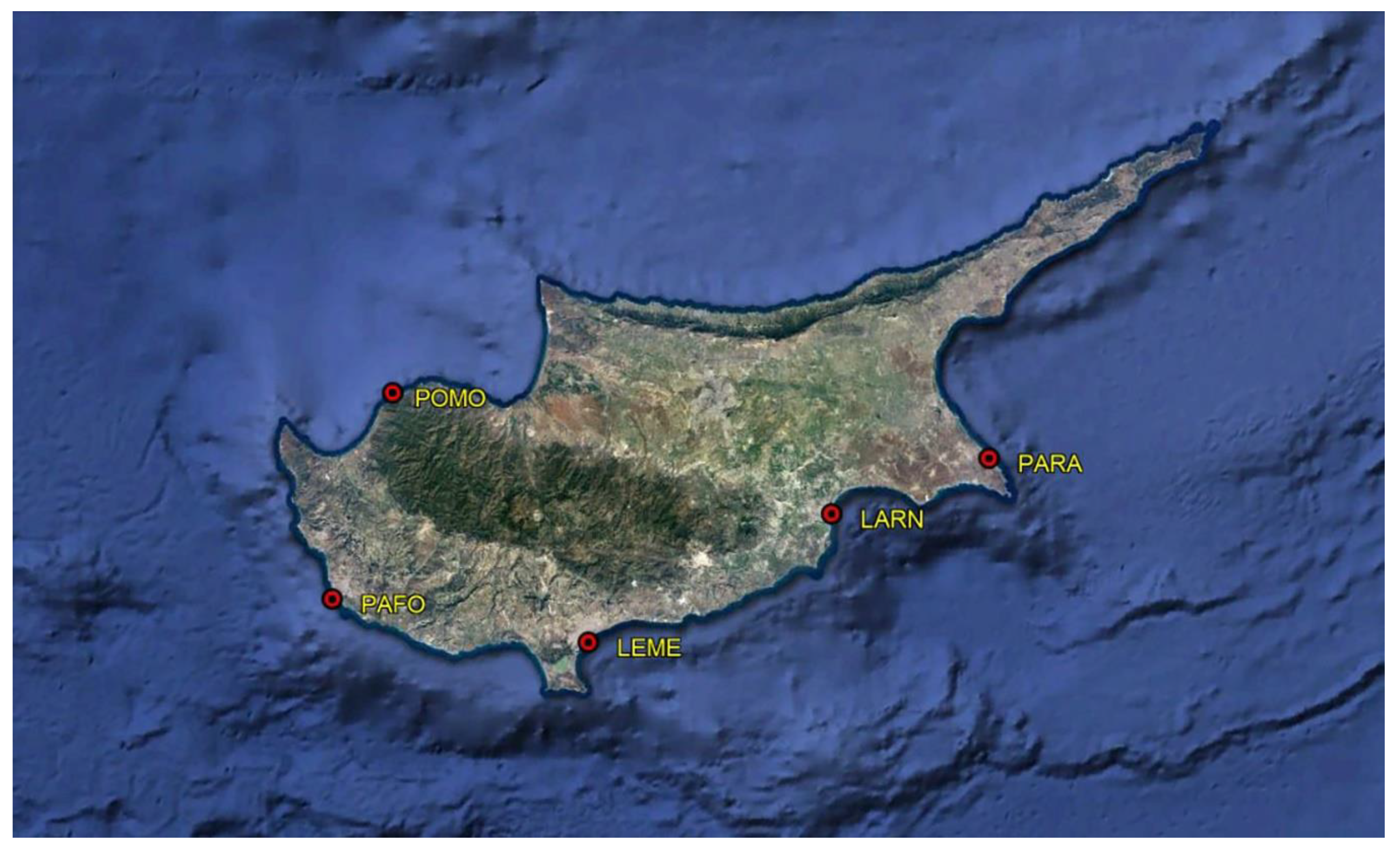
• A description of the Cyprus National TG Network (PYTHEAS) and the processes that were involved during the establishment of the infrastructure;
• The determination of local tidal data in Cyprus using sea-level measurements for the period 2017–2019;
• The transfer of the tidal data to the reference TG station in Limasol.

2. Methodology

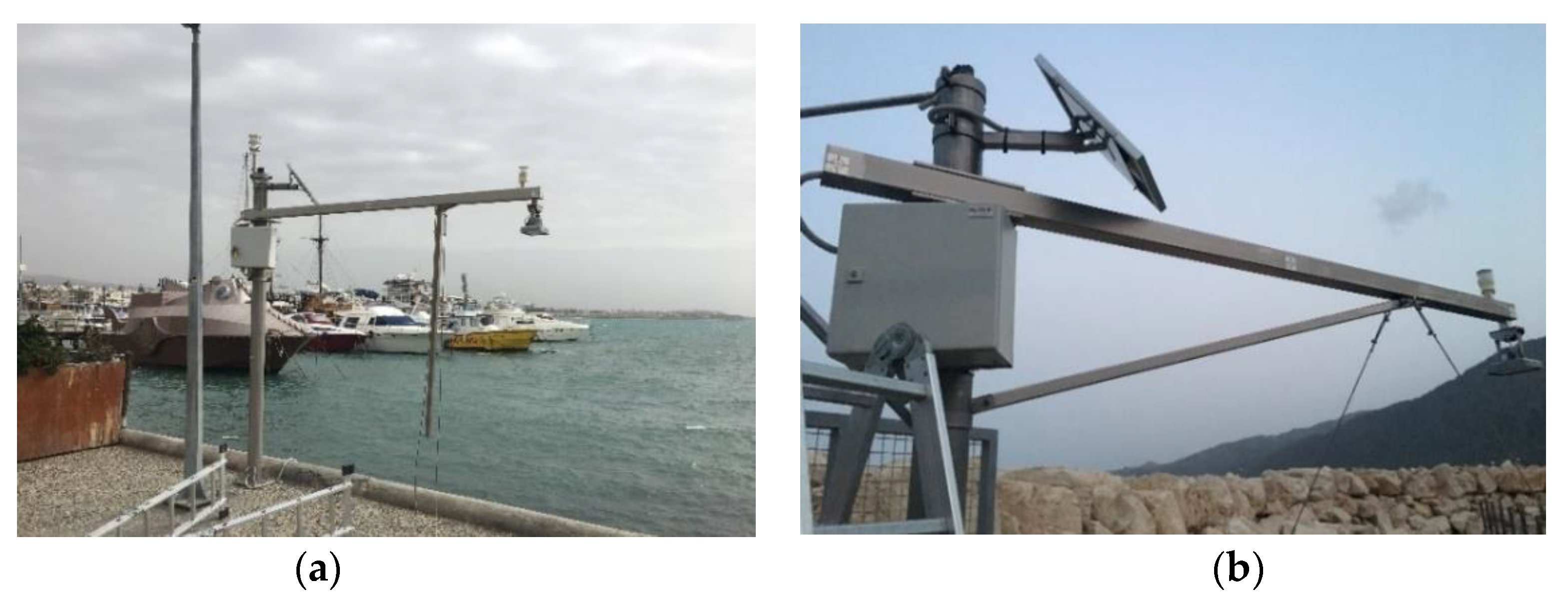
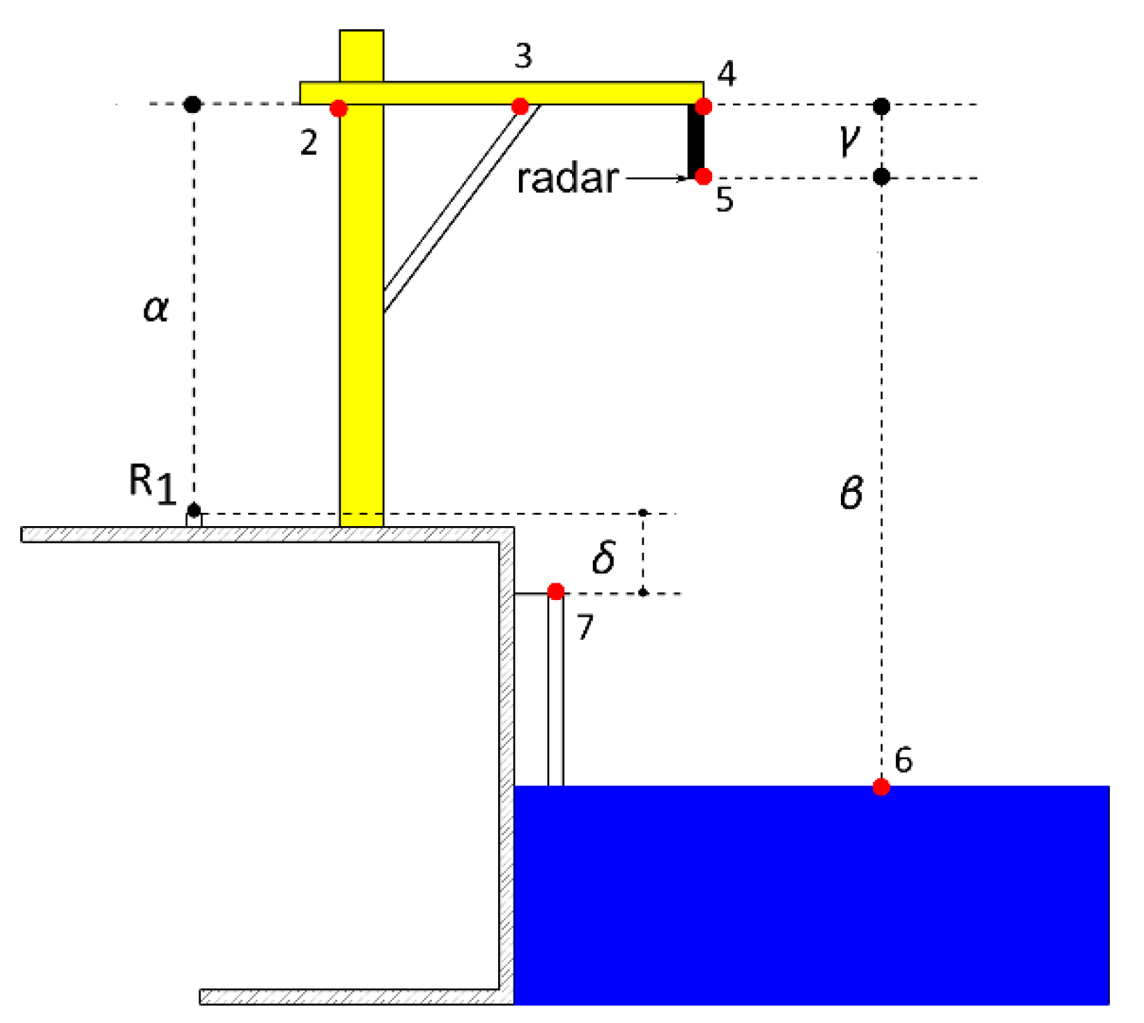
2.1. The Establishment of the National Tide Gauge Station Network (PYTHEAS)

The national network of tides gauges, PYTHEAS, has been established by the Department of Lands and Surveys (DLS) and Cyprus University of Technology (CUT) in the context of the research program THALCHOR2. PYTHEAS includes strategic locations along the coastline of the Republic of Cyprus. In total five integrated measuring stations have been installed in Limassol (CUT), Larnaca (DLS), Paphos (DLS), Pomos (DLS) and Paralimni (DLS). Each integrated station consists of a tide gauge, a weather station, a GNSS reference station, a staff gauge, and auxiliary sensors to measure additional parameters, such as water temperature.

For this infrastructure, radar tide gauges were eventually selected since they combine accuracy, low energy consumption, and low-cost maintenance. Furthermore, radar TGs are not affected by adverse weather conditions and the volume of materials carried by the measured water body, since they do not establish direct contact with water. Radar TGs consist of sensors that measure the instantaneous level of the sea using pulse wave technology for remote measurements. The TG ends in a solid rectangular sensor housing that includes two antennas used for transmission and reception of pulses (see Figure 2). For each respective measurement, pulses are transmitted to the surface of the water, which is reflected to the sensor receiver. The time delay between the broadcast and the reception is proportional to the distance between the sensor and the water surface [12]. Such sensors can be mounted on the side of a bridge or pier or be mounted on a custom platform. In the case of PYTHEAS, all five TGs are using the OTT RLS radar water-level sensor. The latter has been positioned in a specifically designed stainless steel mast configuration to account for maximum stability and convenience in maintenance processes (see Figure 2) and to accommodate all supporting sensors.

The OTT RLS radar water-level sensor enables water-level measurement with an accuracy of ±3 mm from a height ranging from 0.4 m to 35 m. The sensor has been set up to record sea level every 1 min. Note that the OTT RLS outputs filtered values derived from 20 Hz raw measurements [12]. Each integrated TG includes weather stations. These sensors observe five parameters; temperature, relative humidity, air pressure, wind direction and speed. The Limassol (LEME) station is equipped with the Lufft WS500 weather station, while the other four are using GILL MaxiMet GMX500 (see [13] for detailed specifications). The integrated station configurations are illustrated in

Table 1. The sensors that comprise the integrated tide gauge (TG) stations of the PYTHEAS network.

Station	Radar TG	Weather Station	GNSS Receiver	GNSS Antenna
LARN	OTT RLS	Gill MaxiMet GMX500	Trimble® Alloy	Trimble® Zephyr 3
PAFO	OTT RLS	Gill MaxiMet GMX500	Trimble® Alloy	Trimble® Zephyr 3
POMO	OTT RLS	Gill MaxiMet GMX500	Trimble® Alloy	Trimble® Zephyr 3
PARA	OTT RLS	Gill MaxiMet GMX500	Trimble® Alloy	Trimble® Zephyr 3
LEME	OTT RLS	Lufft WS500	Leica GRX 1200 + GNSS	Leica AR25

.

All integrated TG stations are equipped with GNSS reference stations and antennas to perform checks on local deformation and tie the TG reference points (benchmarks) to the national data. The methodology for referencing the tide gauges, the establishment and the referencing of the benchmarks with the local vertical reference system were carried out as follows:

Initially, official benchmarks of the national datum were sought in close proximity to the TGs. After consultation with the DLS, official benchmark reports were provided to CUT to facilitate the process. Consequently, each benchmark was visited to assess its condition. Note that these benchmarks may have been established up to 55 years ago. Therefore, there was a considerable chance that they would be missing (e.g., covered by soil) or destroyed. In the case of missing benchmarks or the establishment of new stations (i.e., the Limassol (LEME) tide gauge), a new reference benchmark was established along with, at least, two additional control benchmarks. The implementation of benchmarks was based on the following criteria:

• Accessibility: The benchmark must enable easy and unobstructed access for future geodetic and surveying works.
• Resilience: The benchmark must be installed at a location with the least chance of destruction or future obstruction.

According to the above two criteria in each tide gauge location, a benchmark was installed near the tide gauge, usually at the pier near the instrument and at least two control benchmarks in the wider study area, in nearby static constructions. The benchmarks used in the infrastructure are two-inches wide levelling marks with datum point made from high-quality bronze alloy. Their installation involved special drilling with countersink drillbits and anchoring using superior epoxy resin to ensure resilience over time and stability (see Figure 3). Note that all benchmark positions were recorded in a specifically designed e-form, which was delivered to DLS.

Subsequently, a mast alignment check was carried out on the tide gauge mounting platforms. This check is considered important as the main mast may gradually be skewed. Note that during maintenance, the horizontal mast is detached from the platform and rotated towards the ground (see Figure 4a). Therefore, its weight may introduce skewness, which may affect the accuracy of the sea-level measurements. Concordantly, alignment control points in the form of reflective adhesive targets, or engravings, were placed in three specific positions along the length of the mast (beginning, middle and end) in each tide gauge (see Figure 4b and points 2–4 in Figure 5). Finally, the height differences between the alignment control points were indirectly determined by means of an industrial-grade total station, namely Topcon MS05AXII (0.5” angular and ±0.5 mm +1 ppm linear precision).

Furthermore, significant control points to connect the tide gauge reference benchmark (e.g., $R_1$), the staff gauge and the radar sensor were established on the mounting platform according to Figure 5. All offsets (or height differences) were measured on-site.

The knowledge of the above offsets along with the MSL (or β) leads to the estimation of the orthometric height of the tide gauge reference benchmark (e.g., $R_1$) using the following equations:

$$H_{R_1}=\beta +\gamma -\alpha$$

(1)

or

$$H_{R_1}=S{G}^{MSL}+\delta$$

(2)

In Equation (2), the term $S{G}^{MSL}$ refers to the staff gauge reading that corresponds to Mean Sea Level. Equation (2) may be used in cases where the TG is regularly calibrated with respect to the staff gauge, and the latter is not moved.

Tying the reference and control benchmarks of each TG to the current national vertical datum (LVD93) was carried out by means of two-way differential leveling between the TG benchmarks and the nearest national LVD93 benchmark established by DLS. Concordantly, the height differences between the reference and control benchmarks in each TG station were measured. Using multiple benchmarks enables the control of the reference benchmark for the occurrence of local deformation (e.g., quay wall settlement or potential scouring phenomena). Additionally, control benchmarks may serve as reference benchmark alternatives in the event of intentional or unintentional benchmark destruction.

Furthermore, the determination of offsets enabled the tie of the TG reference benchmarks to global reference frames, such as the International Terrestrial Reference Frame 2014 (ITRF2014), since the eccentricities of the GNSS antenna reference point (ARP) with respect to the TG reference benchmarks are known. Therefore, the TG reference benchmarks positions were initially estimated using static GNSS observations at the beginning of the project with respect to the International GNSS Service (IGS) permanent station NICO, which is in Nicosia, CY using final orbit and clock products. Daily position estimations will be carried out upon the finalization of the DLS TG stations’ telemetry system.

2.2. Determination of Tidal Levels

The determination of tidal levels was carried out using in-house software developed in MATLAB. The basic workflow can be illustrated in Figure 6. The overall software consists of three main modules: quality control (QC), Interpolation Module (IM) and computation and plotting (CP). Based on this processing chain, the raw data are imported in the QC Module for an initial assessment of the recorded observations. According to specific criteria, which are described in Section 2.2.1, the invalid values are flagged and removed from the dataset. Initially, the IM checks the records for any flagged values and attempts to replace them by means of linear interpolation. To date, the maximum threshold of the attempted interpolation is up to 60 values (1 h). If it is greater, then the attempt to interpolate is abandoned and the module halts. The resampling occurs should for some technical logging issue, the sampling rate of the TG changes and becomes irregular. In this case, the Interpolation module will attempt to reduce the measurements to the same sampling rate, within the 1 h threshold. The data are then checked a second time for any remaining discrepancies. Consequently, the sea-level and meteorological data are averaged from 1 min to hourly. The latter are used in the determination of the tidal data. Furthermore, the software has the ability to automatically generate the appropriate plots, such as the illustration of the sea-level time series, the tidal levels vs. the moon phases, and the de-tided results as illustrated in Figure 6.

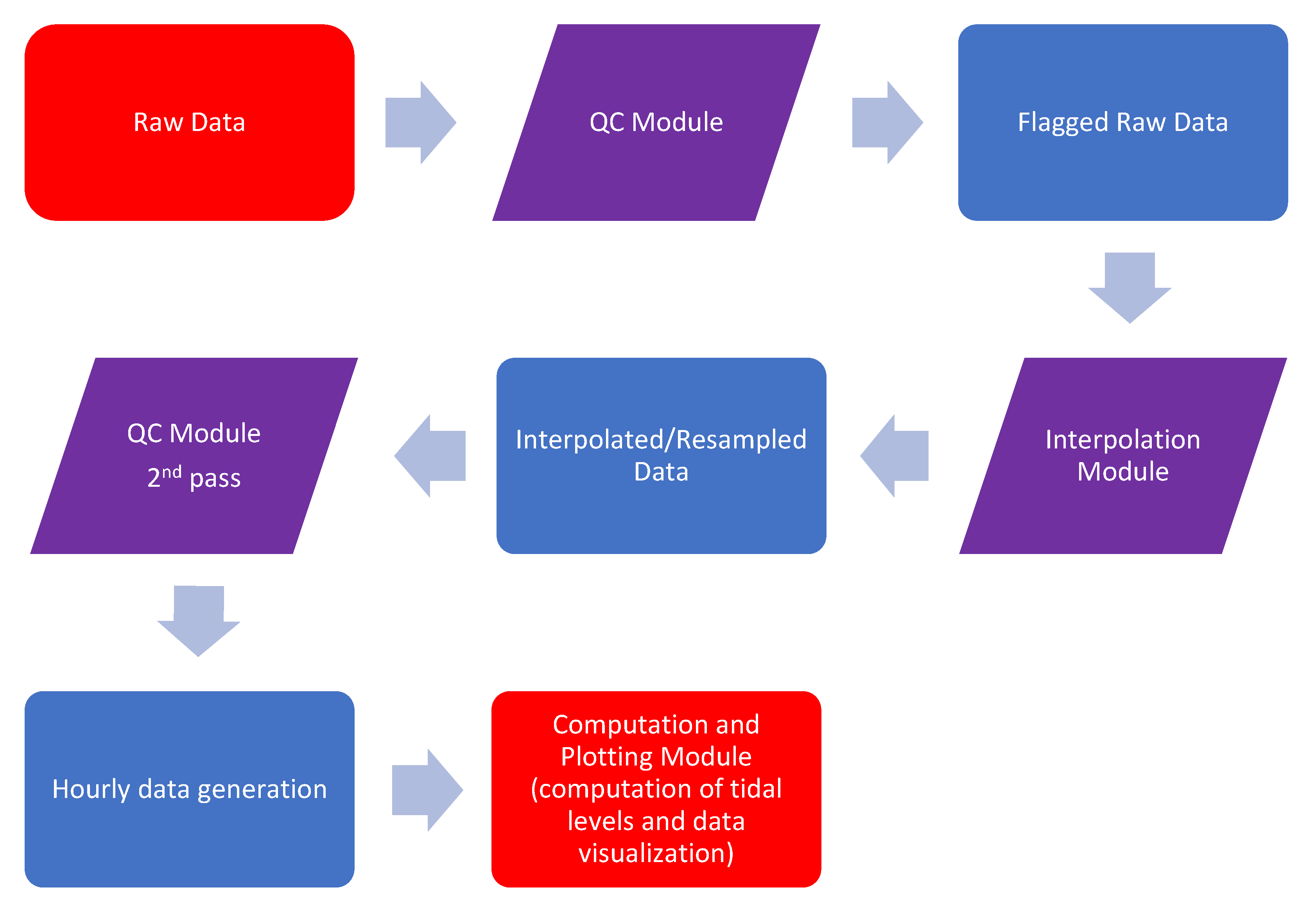
2.2.1. TG Data Pre-Processing and QC

A basic prerequisite for the successful determination of tidal levels is the integrity and reliability of the collected dataset. The sea-level data processing involves several stages of pre-processing of the raw observables before the initialization of the computation phase.

The raw data were quality checked using a modified quality control procedure based on the workflow described in [14]. Initially, sea-level and meteorological data were checked for any large-scale gaps, which are due to serious operating issues of the tide gauge integrated system or an extended power outage. Consequently, the data were then checked for potential smaller-scale data gaps due to accidental data logger errors or occasional storage problems. Additionally, data are checked for sensor malfunctions (both meteorological and sea-level measurements), which are manifested as “zero” recordings in the data, across the whole spectrum of the sensor measurements.

Then, the following checks are carried out using empirical parameters and thresholds:

• Tide gauge stability check: A time threshold of 5 min was defined, as suggested in [14] during which, if the value of the sea-level height remains constant then it indicates a structural instability of the tide gauge. In essence, the software scans for the occurrence of identical sea-level values over the specified timespan. This assessment is mostly applied to stilling well gauges. However, for the sake of completion, it was incorporated in the QC module.
• Outlier detection check: Large outliers are removed by specifying minimum and maximum thresholds. Significantly low or high values usually occur in cases of obstruction of the tide radar (e.g., a boat parking directly below the sensor) or some extreme event (e.g., storm surge). In such cases, outliers (blunders) will appear for a limited amount of time and will exhibit no periodicity. The thresholds initially used in this research were set as the upper and lower staff gauge limits. At the same time, a check is performed for any sudden change in the gradient of the data, which can be an indication of invalid measurements.

Consequently, values that did not meet the specified conditions were removed from the dataset and an attempt was made to fill the gaps by means of linear interpolation where possible. Note that the replacement of invalid values via linear interpolation was carried out for a small period of time to avoid distortion of the time series gradient respecting the time threshold mentioned in Section 2.2. Finally, the data were averaged from 1 min, which is the nominal observation recording interval to hourly.

2.3. Estimation of the Astronomical Impact and Computation of Tidal Levels

In this research, the astronomical impact on the computation of the tidal levels was estimated using the Doodson X0 filter. The Doodson X0 filter belongs to the Finite Impulse Response (FIR) filter family and was originally proposed by Doodson [15,16], and expanded by Pugh [17], along with other slightly different variants from various authors. The Doodson X0 filter is a simple filter that aims to remove the effect of the tidal energy in the sea-level measurements. It is a symmetrical filter, so no phase changes are calculated in its mathematical formula and it is one of the most commonly used de-tiding filters used on tide gauge data. The formula used to compute a filtered value is the following [18,19,20]:

$$X_F\left(t\right)=F_{0}X\left(t\right)+{\displaystyle \sum }_{m=1}^M{F}_m\left[X\left(t+m\right)+X\left(t-m\right)\right]$$

(3)

where the calculated values of $X_F\left(t\right)$ are normalized with the selection of M = 19 values from both sides of the pivot (being the 00:00 h of each calendar day). The $F_m$ weights used are:

$$\frac{101001011020110211202112011020110100101}{30}$$

(4)

According to [21], the Doodson X0 filter eliminates 99.94% of the tidal energy at semidiurnal frequencies, 99.79% at diurnal frequencies and 99.38% at overtide frequencies.

Note that the tide in Cyprus is characterized as semi-diurnal (see Figure 7) with its characteristic 2 high and 2 low waters per each tidal day.

For the calculation of the MSL, an arithmetic average of the hourly values of the data was produced for each station (Equation (1)), and the result was used as a tidal datum, according to which the other tidal levels are referenced [22,23].

$$MSL=\frac{{\displaystyle \sum }{h}_i}{n}$$

(5)

where: $h_i$ the hourly sea-level height observations and $n$ their number.

Ideally, tidal levels are estimated using a full tidal epoch, which spans approximately 19 years of measurements, to account for the full moon nodal cycle and declinations relative to Earth’s equatorial plane. However, this research performs a first estimation of tidal levels using the available data [24,25].

The Mean High (MHW) and Mean Low Water (MLW) tidal levels were calculated respectively by the arithmetic mean of the two high and two low water levels of each tidal day (semi-diurnal tide), while the Mean Higher High (MHHW) and Mean Lower Low Water (MLLW) levels were determined by the highest and lowest water value observed each tidal day. The Higher High Water (HHW) and Lower Low Water (LLW) were estimated by the highest and lowest value of the dataset, respectively. Furthermore, data for each station were separated and processed in lunar months, to account for the successive Moon phases, since the lunar attractive force combined with the solar contribute to the spring/neap tide cycle [22]. The mean tide level was defined by the average of the Mean High Water and Mean Low Water of each tidal day.

In the final step of data processing, the filtered data were plotted against the unfiltered and their difference provides an insight into the influence of the tide-generating forces exerted by the celestial bodies. The filtered data contain, predominantly, non-tidal energy and meteorological residuals and are closer to an actual water-level record [26,27].

2.4. Tidal Data Transfer

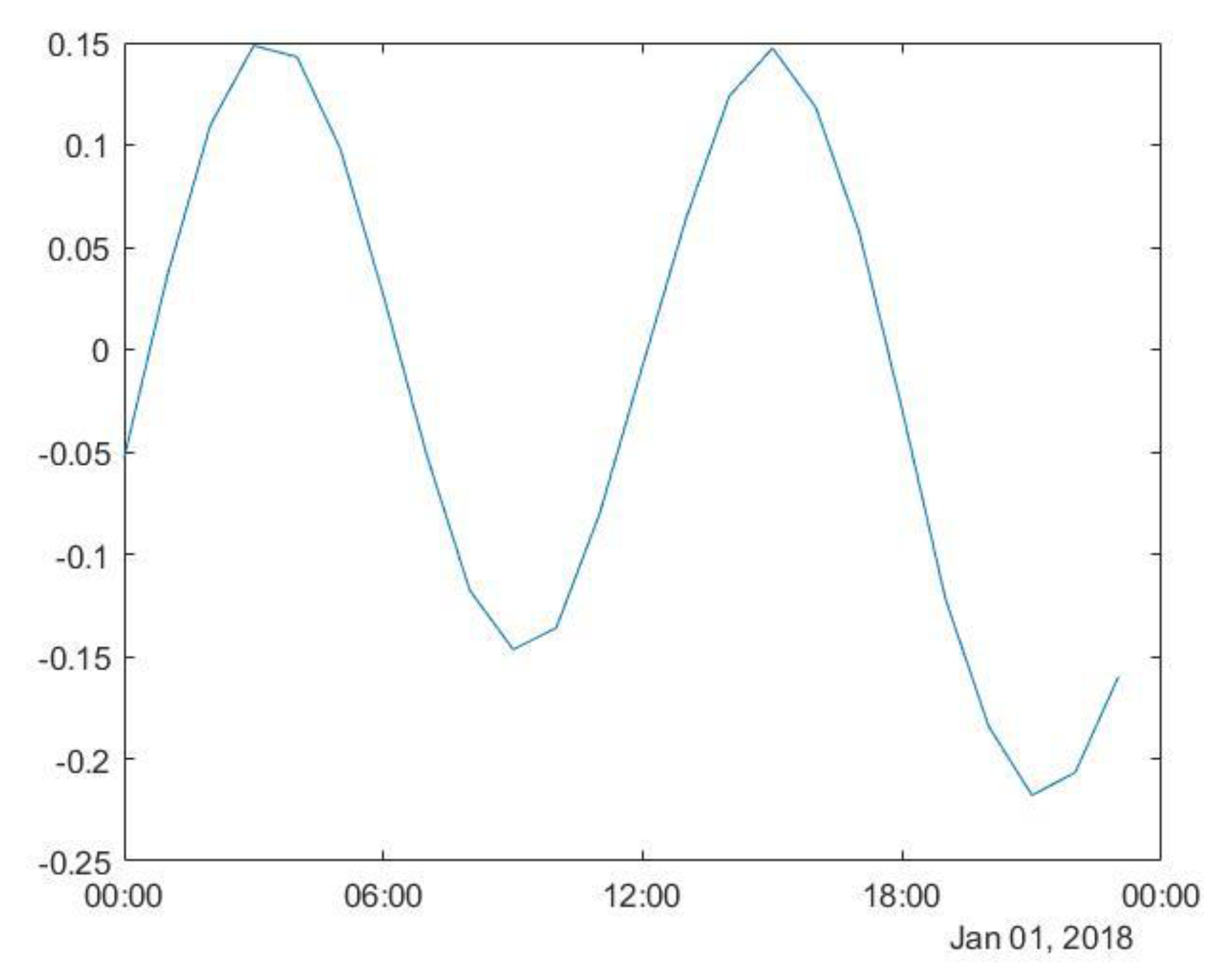
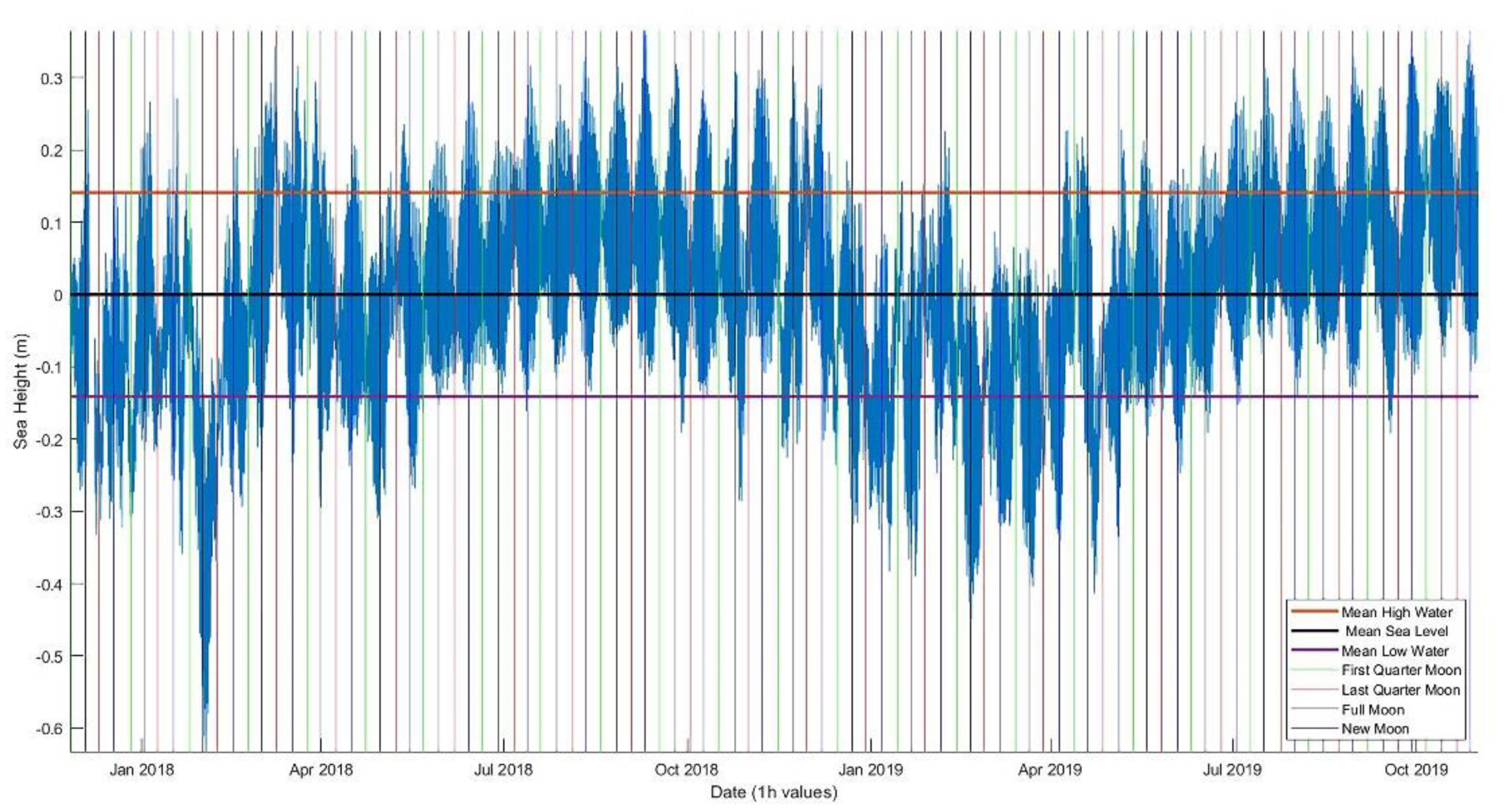
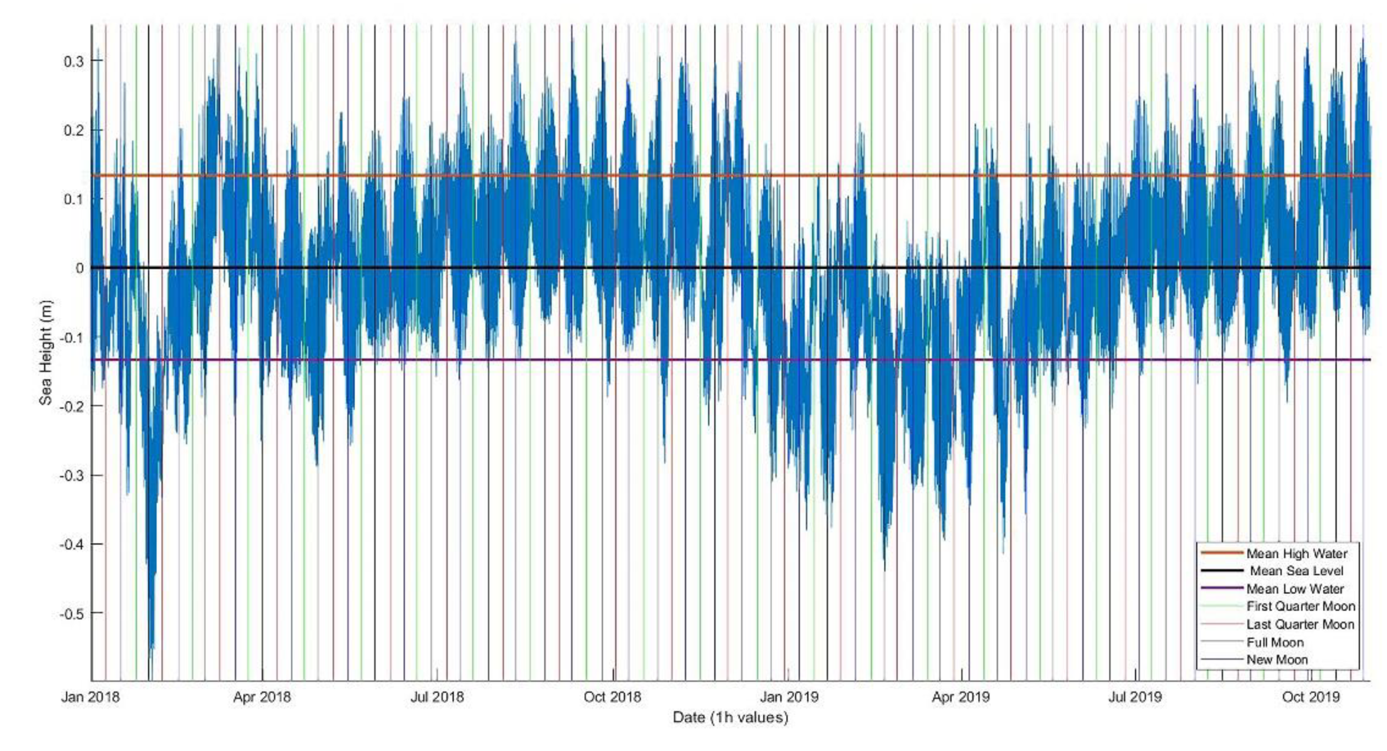
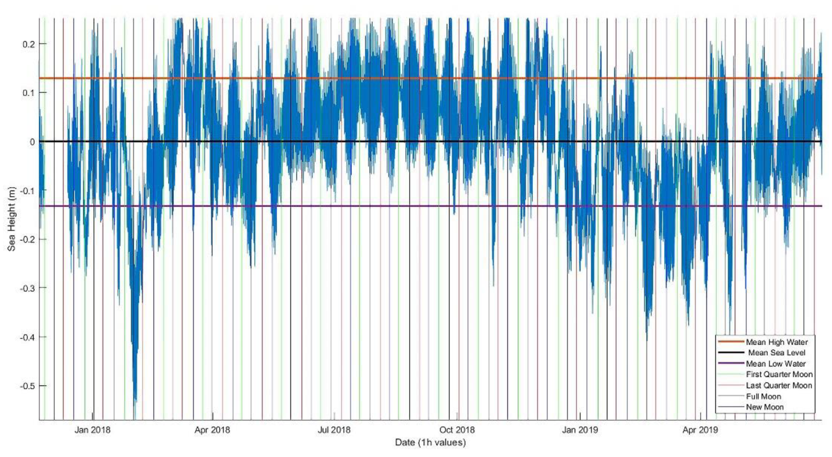
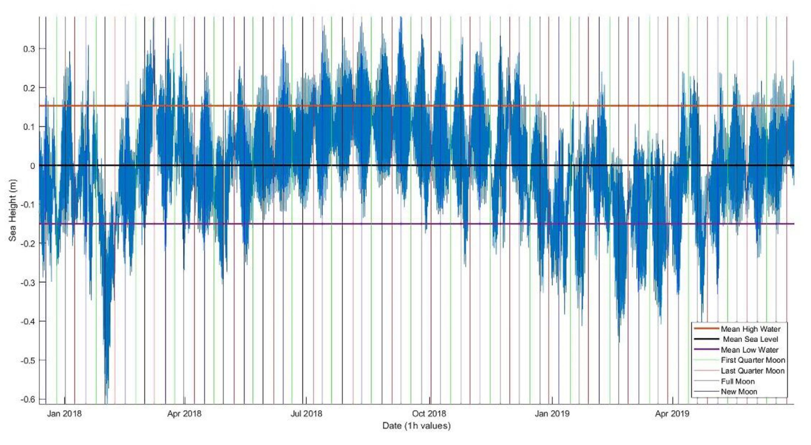
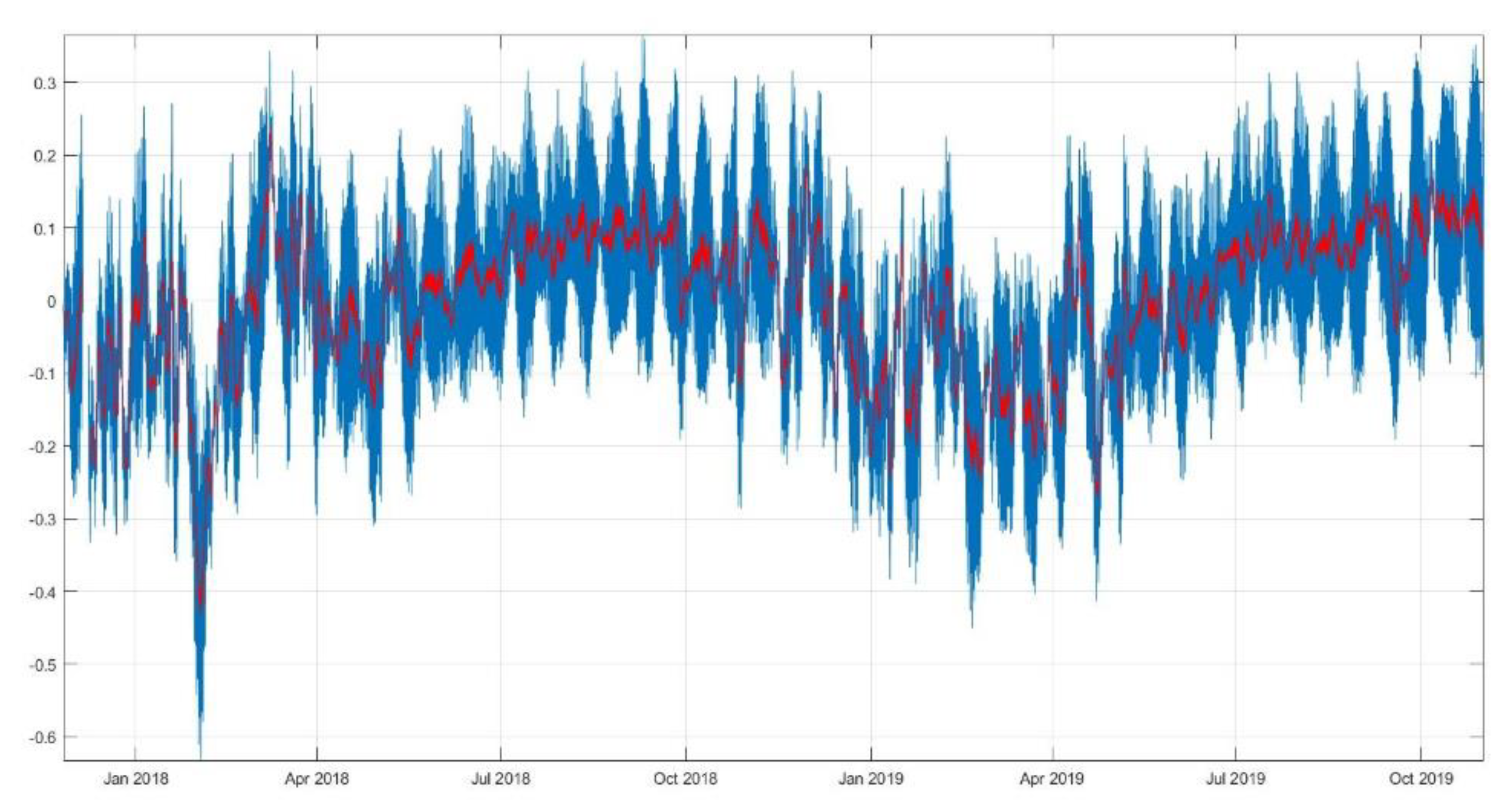
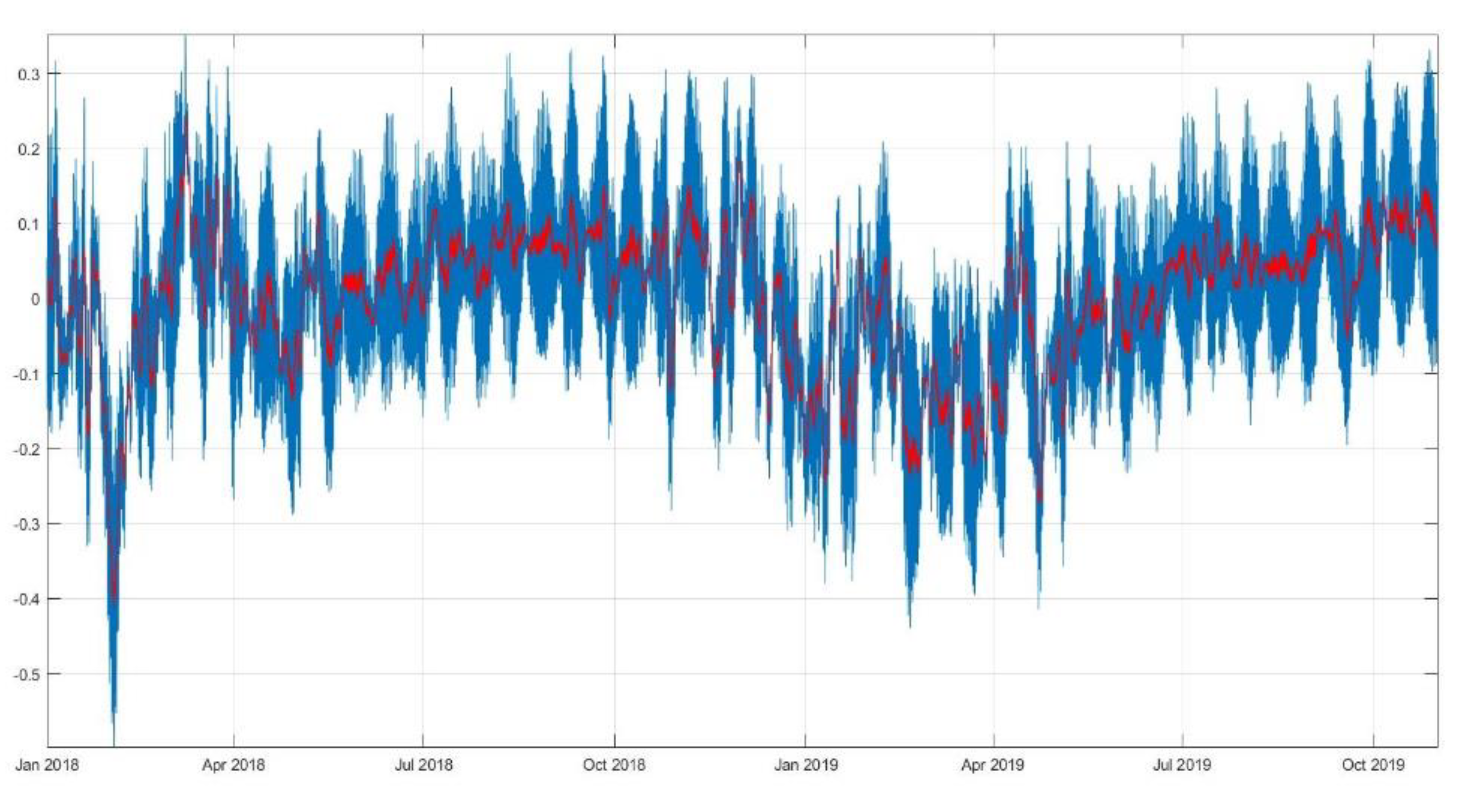
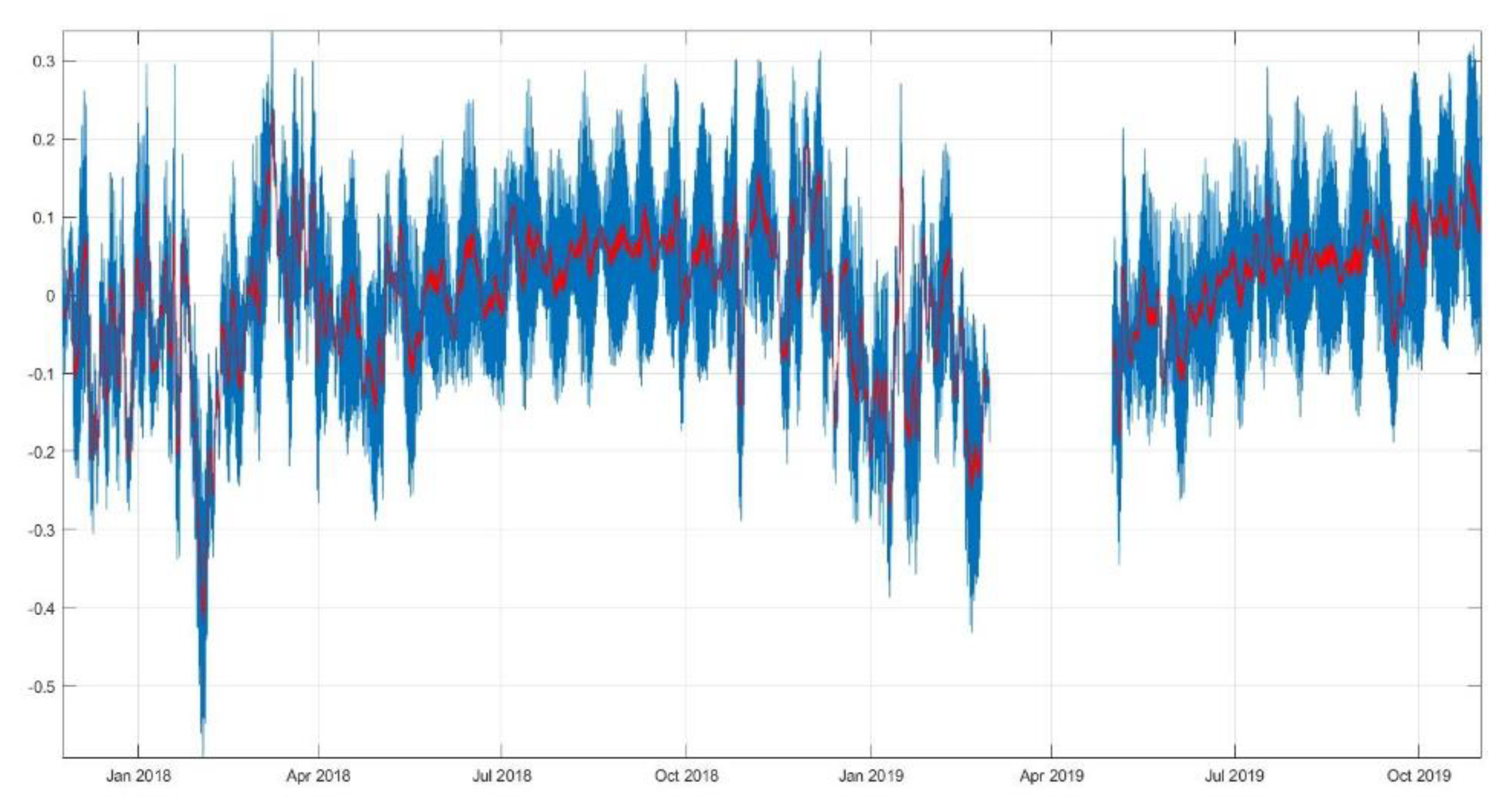
The comparison of the results between the tide gauges of the PYTHEAS network was based on two assumptions. First, it is assumed that the water levels between the reference TG station (which is LEME in our case, since it had a smaller amount of errors as shown in

Table 2. Dataset quality assessment (QC) results.

Station	Observation Period	Number of Observations	ACCEPTED	REJECTED
LARN	21/11/2017 00:00–31/10/2019 23:59	1015859	1013623 (99.88%)	2236 (0.22%)
PAFO	24/11/2017 00:00–31/10/2019 23:59	930334	929073 (99.87%)	1261 (0.13%)
POMO	22/11/2017 00:00–30/06/2019 23:59	808688	794725 (98.83%)	13963 (1.7%)
PARA	13/12/2017 00:00–30/06/2019 23:59	812301	811002 (99.84%)	1299 (0.16%)
LEME	01/01/2018 00:00–31/10/2019 23:59	963228	963167 (99.99%)	61 (0.006%)

) and the receiving station undergo similar deviations from the perceived norms for the tidal epoch under study. Secondly, it is presumed that the difference in the proximity of each receiving station from the reference station has a negligible impact on the mix of astronomical and meteorological forces since they measure the same water body. By averaging the data to hourly values, we applied the procedure of MSL, and other tidal datum transfers as described in [22] using the following equation:

$$MS{L}_{target}=\left(MMS{L}_{target}-MMS{L}_{LEME}\right)+MS{L}_{LEME}$$

(6)

where $MS{L}_{target}$ is the MSL of the target or receiving station, $MMS{L}_{target}$ and $MMS{L}_{LEME}$ are the Monthly Sea Level of the receiving and reference station respectively, and the $MS{L}_{LEME}$ the estimated and accepted MSL of the reference station, which is referenced to a local staff gauge installed next to the TG (see Figure 2).

Similarly, the mean tide-level datum was transferred using the same method as in Equation (7):

$$MT{L}_{target}=(MMT{L}_{target}-MMT{L}_{LEME})+MT{L}_{LEME}$$

(7)

3. Results

As mentioned in Section 3, the raw data were preprocessed to remove invalid observations that were dispersed within as a result of sensor issues, radar obstruction or any other event that might cause instability to data logging. The QC results are summarized in Table 2.

In detail, the quality control procedure of the data yielded the following results:

Larnaka (LARN): A gap of 4.5 days (6541 potential measurements) was detected in the data array. Out of the 2236 invalid values, 285 were due to station sensor errors, 85 were due to recording errors, and 1666 exceeded the specified thresholds.

Pafos (PAFO): A gap of 60 days (87,641 potential measurements) was detected in the data array. Out of 1261 invalid values, 84 were recording errors and 1248 were off the thresholds.

Pomos (POMO): A gap of about 24.5 days (35,152 potential measurements) was detected in the data array. Of the 13,963 incorrect measurements found, 83 were recording errors, 4314 were due to station sensor failure and 5320 values exceeded the specified thresholds.

Paralimni (PARA): A gap of approximately 23 h (1299 potential measurements) was detected. Out of the 1029 incorrect measurements, 8 were attributed to sensor failure and 1021 were off the threshold.

Limassol (LEME): A gap of approximately 2 h (132 potential measurements) was observed. Of the 61 incorrect measurements, 20 were for recording errors, 21 for sensor errors, and 20 were off the threshold.

It is worth noting that no stability errors were found in any of the stations, a fact that emphasizes the structural integrity of the tide gauges. According to the above, the most reliable data logging is performed by the LEME and PAFO TG stations (with the LEME station having an error rate of less than 0.02%) while the most issues were recorded at the POMO station. It is noted that this particular station faced technical issues with the sensor. Furthermore, the water-level sensor is installed over shallow waters, with rocks at the bottom and, exactly at the corner of the quay and the wave breaker. The aforementioned factors favor the occurrence of extreme values, especially during intense weather conditions, i.e., strong winds generating waves.

In the figures below (Figure 8, Figure 9, Figure 10 and Figure 11), a visual representation of the referenced and de-tided data is presented. It is important to note that the tidal data are calculated for each tidal gauge locally, and an overview of the tidal datum differences between each station and the LEME reference station is included [28].

According to Figure 8, Figure 9, Figure 10, Figure 11 and Figure 12, there is a strong seasonal signal in all tide gauge station data, as there is a common downward trend in October–April, while between April until October, the sea height tends to increase. These fluctuations are expected since the sea height, apart from the astronomical component, is also influenced by other factors such as the wind pattern and intensity, changes in the sea temperature that relate to thermal expansion and in salinity (saline contraction) [29]. The sudden drop in sea level at the beginning of Feb 2018 can be explained by the increase in the observed pressure as recorded by all TG stations. Specifically, the mean daily pressure changed from 1008 hPa (in 28.01.2018) to 1026 hPa (in 05.02.2018).

Table 3. The calculated tidal levels of the PYTHEAS TG network stations. The results are in meters.

Station	MSL	MHW	MLW	MHHW	MLLW	HHW	LLW	MTL	ATI
LARN	1.073	0.141	−0.141	0.163	−0.156	0.3651	−0.6335	0.141	0.084
LEME	1.353	0.133	−0.133	0.155	−0.150	0.3522	−0.5990	0.133	0.084
PAFO	1.194	0.136	−0.135	0.159	−0.151	0.3381	−0.5929	0.135	0.078
POMO	1.022	0.129	−0.132	0.149	−0.149	0.3175	−0.5665	0.130	0.066
PARA	1.195	0.153	−0.150	0.177	−0.169	0.3825	−0.6142	0.151	0.093

presents an overview of the Mean Sea Level (MSL), Mean High Water (MHW), Mean Low Water (MLW), Mean Higher High Water (MHHW), Mean Lower Low Water (MLLW), Lower Low Water (LLW), Higher High Water (HHW), Mean Tide Level (MTL) and Astronomical Tide Impact (ATI) as computed by processing the available data. The MSL is referenced to the staff gauge of each station, while the other tidal data were referenced to the MSL of the corresponding TG station. With respect to the MSL, the highest computed value was seen in the LEME station (installed at the Limassol old port) and the lowest in POMO station which is located at the docks of the Pomos village, in the Northeastern Paphos district. The highest tidal range is found at the PARA station (0.303 m) in which the observed tidal datum values are relatively large, while the lowest is found at the POMO station (0.261 m). Regarding the MHW, MHHW, MLLW, MTL the largest values are found at the PARA station with the largest MLW observed at the LARN station though (located at Larnaka dock, South Cyprus). Consistently, the larger tidal levels are observed south of Cyprus and the smaller at the north of the island, with the levels observed in the west (PAFO station, located at the Paphos docks) being in-between.

Table 4. Mean difference between the reference station datum (LEME) and the receiving stations. The results are expressed in meters.

Station	Mean ΔMSL	Mean ΔMTL	ΔMSL Std. Deviation	ΔMTL Std. Deviation
PARA	0.011	−0.012	0.072	0.074
PAFO	−0.016	−0.013	0.091	0.072
POMO	−0.009	−0.012	0.071	0.074
LARN	−0.010	−0.014	0.089	0.044

illustrates the mean differences between the accepted MSL and MTL datum of the LEME reference TG station and the receiving stations. Note that LEME’s MSL and MTL are referenced to the local staff gauge zero. The difference was computed by subtracting the receiving station data (referenced to the LEME datum) from the data that were referenced to the local staff gauge according to Equation (6). Overall, the sea-level variations occur in an almost uniform manner in all stations, based on Figure 8, Figure 9, Figure 10, Figure 11 and Figure 12, with the temporal appearances of spring/neap tide cycle and high/low water occurring at nearly identical times. According to Table 4, the difference between the MSL and MTL of the reference station’s staff gauge and the receiving station’s is approximately 1 cm lower, with PARA TG being the only exception, which is nearly 1 cm higher. This is expected given that all TGs are installed at nearly identical surroundings (ship docks), using similar design and installation.

Table 5. The Lowest Low Water (LLW) tidal datum (middle column) adjusted to the Mean Sea Level (MSL) of the LEME station (right column). The results are expressed in meters.

Station	LLW According to Local MSL	Adjusted LLW
PARA	−0.614	−0.603
PAFO	−0.593	−0.609
POMO	−0.567	−0.575
LARN	−0.633	−0.644

illustrates the referenced LLW levels for each station to the LEME MSL datum (adjusted LLW).

Finally, Figure 13, Figure 14, Figure 15, Figure 16 and Figure 17 present the de-tided data vs. the observed sea-level time series. The impact of the celestial tide generating forces on the regional sea level is apparent. The astronomical tide impact on the sea height in percentage, according to Table 3 above, is about 59% (MTL–ATI), while the remaining 41% is attributed to meteorological influence. The mean tide (MTL) for all stations is 13.8 cm, although this preliminary result should be viewed with caution since an extreme event (as the one that occurred in February 2018) may potentially bias the computed means.

4. Discussion

PYTHEAS, the new national infrastructure of permanently integrated tide gauge stations, was described in this research. Five stations were established along the coastline of the Republic of Cyprus recording sea-level, meteorological and position information to determine tidal levels and support critical activities such as Maritime Spatial Planning, hydrographic surveys and the national geodetic infrastructure. An initial estimation was carried out using the available data from all five TGs. Using a common tidal datum, a difference in the MSL of about 1 cm was observed between the reference station and the receiving stations. The tidal range is between 0.26–0.30 m, which is classified as a micro-tidal range. The latter was expected if we take into consideration the volume of water and the geography of the sea it resides in. In short, with the available data, it can be concluded that the tides around the sea of the Cyprus Republic are quite small and quite characteristic of the Mediterranean Sea. With a common datum established using the available observations, an effort will be made to establish the direction of the trend of sea height.

Evidently, the proposed methodology and infrastructure will enable a thorough study of the MSL variability throughout the coming years. This study will highlight the link between the MSL and the coastal erosion/submersion regime in Cyprus. In the context of MSP, the exact relation between coastal erosion and the MSL needs to be determined and examine whether it is additive or multiplicative or even subtractive to the erosion or accretion to the coasts of Cyprus. Consequently, potential dangers, susceptible areas or exploitation opportunities will be identified. A constant rise of the MSL will intensify the existing severe erosion issues seen in cities, which exhibit a high degree of urban development and construction activity (e.g., city of Limassol) at their coastal zone. The latter will be more vulnerable to high-energy waves reaching further up the shore, especially in extreme events such as storm surges, and flooding. Furthermore, the analysis of the TG observations collected by the PYTHEAS network, along with information on the coastal history of Cyprus, will be used for the calculation of the ratio of MSLR/erosion as in the case of the U.S. East Coast, where the ratio calculations have yielded that a 10 cm rise in MSL results in a shoreline erosion of 15 cm [30]. The TG’s in situ observations analysis that has been carried out to date, and the development of a modernized vertical reference system, will form the backbone for the systematic analysis of the MSLR and its impact on the Cyprus coastline. Furthermore, the results derived from such an analysis will be used to promote national civil defense strategies, and assist in their incorporation into a successful MSP.

5. Conclusions

PYTHEAS, the national tide gauge network of the Republic of Cyprus, was established by the Department of Lands and Surveys and the Cyprus University of Technology. The main objective of PYTHEAS is the realization of a state-of-the-art infrastructure to support critical activities, such as the implementation of the Maritime Spatial Planning of Cyprus carried out in the framework of THAL-CHOR 2 project. Based on the establishment of the PYTHEAS, the following actions were performed in this research:

• The establishment of a procedure for the physical installation and referencing of TG’s;
• The definition of the methodology for the QC of the observations and the calculation of local tidal data. Α microtidal range of 0.303 to 0.261 was determined and a difference of 1 cm in the MTL and MSL data between the auxiliary stations and the reference TG.
• The definition of a common tidal level, which will be used for the determination of a benchmark to study MSLR and MSL variability;
• The calculation of the astronomical influence, and indirectly, the meteorological residuals that affect the sea elevation of Cyprus. The astronomical influence was estimated to contribute approximately 59% (~8 cm) to sea elevation, while the remaining portion is attributed to meteorological residuals (41% or approximately 5 cm).

The next steps involve the assimilation of more data to determine the major tidal constituents by means of harmonic analysis. These can be utilized for the purpose of forecasting and to provide a more precise calculation of the astronomical impact on the regional sea level. Furthermore, tide gauge observations will be combined with satellite altimetry data for calibration and validation purposes and to augment the MSL estimation in the offshore areas. Evidently, with the advent of PYTHEAS, an opportunity is presented for a coherent study of the tidal levels of Cyprus and the establishment of a modernized vertical reference system.

References

1. Ehler, C.; Douvere, F. Marine Spatial Planning: A step-by-step approach toward ecosystem-based management. In Intergovernmental Oceanographic Commission and Man and the Biosphere Programme; IOC Manual and Guides No. 53; ICAM Dossier No. 6; UNESCO: Paris, France, 2009. (In English) [Google Scholar]
2. Douvere, F. The importance of marine spatial planning in advancing ecosystem-based sea use management. Mar. Policy 2008, 32, 762–771. [Google Scholar] [CrossRef]
3. Coastance. Eu Project Coastance Report Phase B2–B3, Component 3: Regional Action Strategies for Coastal Zone Adaptation to Climate Change; Conseil général de l’Hérault,Pôle Développement Durable, Direction du Développement Littoral et Maritime: Montpellier, France, 2012; pp. 1–3. [Google Scholar]
4. Consortium for Ocean Leadership. Science Requirements for Marine Spatial Planning; Consortium for Ocean Leadership: Washington, DC, USA, 2009; pp. 1–4. [Google Scholar]
5. Ehler, C. A Guide to Evaluating Marine Spatial Plans; MarXiv: Santa Barbara, CA, USA, 2017; p. 41. [Google Scholar]
6. Hadjimitsis, D.; Agapiou, A.; Themistocleous, K.; Mettas, C.; Evagorou, E.; Soulis, G.; Xagoraris, Z.; Pilikou, M.; Aliouris, K.; Ioannou, N. Maritime spatial planning in Cyprus. Open Geosci. 2016, 8, 653–661. [Google Scholar] [CrossRef] [Green Version]
7. UNESCO, IOC. Manual on Sea-level Measurements and Interpretation; Manual Guides, JCOMM Technical Report No. 31; UNESCO: Paris, France, 2006; Volume IV. [Google Scholar]
8. UNESCO, IOC. Manual on sea level measurement and interpretation. In Intergovernmental Oceanographic Commission, Manuals and Guides 14; UNESCO: Paris, France, 1985; p. 83. [Google Scholar]
9. ROSEN, D.S. Medgloss-mediterranean and black sea regional sea level monitoring network: Update of activities and progress. In Proceedings of the 11th Session of the IOC/UNESCO Group of Experts on the Global Sea Level Observing System (GLOSS), Paris, France, 13–15 May 2009. [Google Scholar]
10. Agresti, V. Effects of Tidal Motion on the Mediterranean Sea General Circulation. Ph.D. Thesis, Alma Mater Studiorum Università di Bologna, Bologna, Italy, 2018. [Google Scholar]
11. Bonaduce, A.; Pinardi, N.; Oddo, P.; Spada, G.; Gilles Larnicol, G. Sea-level variability in the Mediterranean Sea from altimetry and tide gauges. Clim. Dyn. 2016, 47, 2851–2866. [Google Scholar] [CrossRef] [Green Version]
12. Operating Instructions Radar Level Sensor OTT RLS. Available online: https://www.otthydromet.com/en/p-ott-rls-radar-level-sensor/6310900192S#resources (accessed on 19 July 2020).
13. User Manual Smart Weather Sensors. Available online: https://www.lufft.com/download/manual-lufft-wsxxx-weather-sensor-en/ (accessed on 19 July 2020).
14. Pérez, B.; Álvarez Fanjul, E.; Pérez, S.; de Alfonso, M.; Vela, J. Use of tide gauge data in operational oceanography and sea level hazard warning systems. J. Oper. Oceanogr. 2013, 6, 1–18. [Google Scholar] [CrossRef]
15. Doodson, A.T.; Warburg, H.D. Admiralty Manual of Tides; HM Stationery Office: Richmond, UK, 1941. [Google Scholar]
16. Doodson, A.T. The Harmonic Development of the Tide-Generating Potential. Proc. R. Soc. Lond. Ser. A 1921, 100, 305–329. [Google Scholar]
17. Pugh, D.T. Tides, Surges and Mean Sea Level; U.S. Department of Energy Office of Scientific and Technical Information: Oak Ridge, TN, USA, 1987.
18. Shirahata, K.; Shuhei, Y.; Takeo, T.; Satoshi, I. Digital filters to eliminate or separate tidal components in groundwater observation time-series data. Jpn. Agric. Res. Q. JARQ 50 2016, 50, 241–252. [Google Scholar] [CrossRef] [Green Version]
19. Parker, B.B. The Response of Massachusetts Bay to Wind Stress. Ph.D. Thesis, Massachusetts Institute of Technology, Cambridge, MA, USA, 1975. [Google Scholar]
20. Pugh, D.; Woodworth, P. Sea-Level Science: Understanding Tides, Surges, Tsunamis and Mean Sea-Level Changes; Cambridge University Press: Cambridge, UK, 2014; pp. 20–21. [Google Scholar]
21. Groves, G.W. Numerical filters for discrimination against tidal periodicities. Eos Trans. Am. Geophys. Union 1955, 36, 1073–1084. [Google Scholar] [CrossRef]
22. Boon, J.D. Secrets of the Tide: Tide and Tidal Current Analysis and Predictions, Storm Surges and Sea Level Trends; Elsevier: Amsterdam, The Netherlands, 2013; pp. 60–66. [Google Scholar]
23. Rossiter, J.R. A routine method of obtaining monthly and annual values of sea level from tidal records. Int. Hydrogr. Rev. 1961, 38, 42–45. [Google Scholar]
24. Foreman, M.G.G. Manual for Tidal Heights Analysis and Prediction; Institute of Ocean Sciences: Patricia Bay, BC, Canada, 1979. [Google Scholar]
25. Consoli, S.; Recupero, D.R.; Zavarella, V. A survey on tidal analysis and forecasting methods for Tsunami detection. arXiv 2014, arXiv:1403.0135. [Google Scholar]
26. Le Provost, C. Ocean tides. In International Geophysics; Academic Press: Cambridge, MA, USA, 2001; Volume 69, pp. 267–303. [Google Scholar]
27. Parker, B.B. Tidal Analysis and Prediction; NOAA Special Publication NOS CO-OPS 3; National Oceanic and Atmospheric Administration: Washington, DC, USA, 2007. [Google Scholar]
28. Godin, G. The Analysis of Tides; No. 551.4708 G6; University of Toronto: Toronto, ON, Canada, 1972. [Google Scholar]
29. Amiruddin, A.M.; Haigh, I.D.; Tsimplis, M.N.; Calafat, F.M.; Dangendorf, S. The seasonal cycle and variability of sea level in the South China Sea. J. Geophys. Res. Oceans 2015, 120, 5490–5513. [Google Scholar] [CrossRef] [Green Version]
30. Leatherman, S.P.; Zhang, K.; Douglas, B.C. Sea level rise shown to drive coastal erosion. Eos Trans. Am. Geophys.Union 2000, 81, 55–57. [Google Scholar] [CrossRef]
Figure 1. PYTHEAS: The national tide gauge network of the Republic of Cyprus.
Jmse 08 00861 g001
Figure 2. The Limassol (LEME) integrated tide gauge station.
Jmse 08 00861 g002
Figure 3. Installation of TG benchmarks using high-quality levelling markers.
Jmse 08 00861 g003
Figure 4. (a) the tide gauge horizontal mast during maintenance, (b) the installation of special adhesive targets along the mast to check alignment.
Jmse 08 00861 g004
Figure 5. Tide gauge significant control points and their offsets.
Jmse 08 00861 g005
Figure 6. The processing workflow for the determination of tidal levels.
Jmse 08 00861 g006
Figure 7. A tidal day plot of Limassol (LEME) station, which illustrates the semi-diurnal tide.
Jmse 08 00861 g007
Figure 8. Local determination of Larnaka (LARN) station tidal levels (horizontal lines) with moon phases (vertical lines).
Jmse 08 00861 g008
Figure 9. Local determination of Limassol (LEME) station tidal levels (horizontal lines) with moon phases (vertical lines).
Jmse 08 00861 g009
Figure 10. Local determination of Pafos (PAFO) station tidal levels (horizontal lines) with moon phases (vertical lines).
Jmse 08 00861 g010
Figure 11. Local determination of Pomos (POMO) station tidal levels (horizontal lines) with moon phases (vertical lines).
Jmse 08 00861 g011
Figure 12. Local determination of Paralimni (PARA) station tidal levels (horizontal lines) with moon phases (vertical lines).
Jmse 08 00861 g012
Figure 13. LARN tide gauge de-tided data. The overlay red line denotes the sea height with the astronomical influence suppressed.
Jmse 08 00861 g013
Figure 14. LEME tide gauge de-tided data. The overlay red line denotes the sea height with the astronomical influence suppressed.
Jmse 08 00861 g014
Figure 15. PAFO tide gauge de-tided data. The overlay red line denotes the sea height with the astronomical influence suppressed.
Jmse 08 00861 g015
Figure 16. PARA tide gauge de-tided data. The overlay red line denotes the sea height with the astronomical influence suppressed.
Jmse 08 00861 g016
Figure 17. POMO tide gauge de-tided data. The overlay red line denotes the sea height with the astronomical influence suppressed.
Jmse 08 00861 g017