Design and Optimization of a Radial Turbine to Be Used in a Rankine Cycle Operating with an OTEC System


Abstract
1. Introduction
2. Turbine Rotor Design Process
2.1. Turbine Design Guidelines
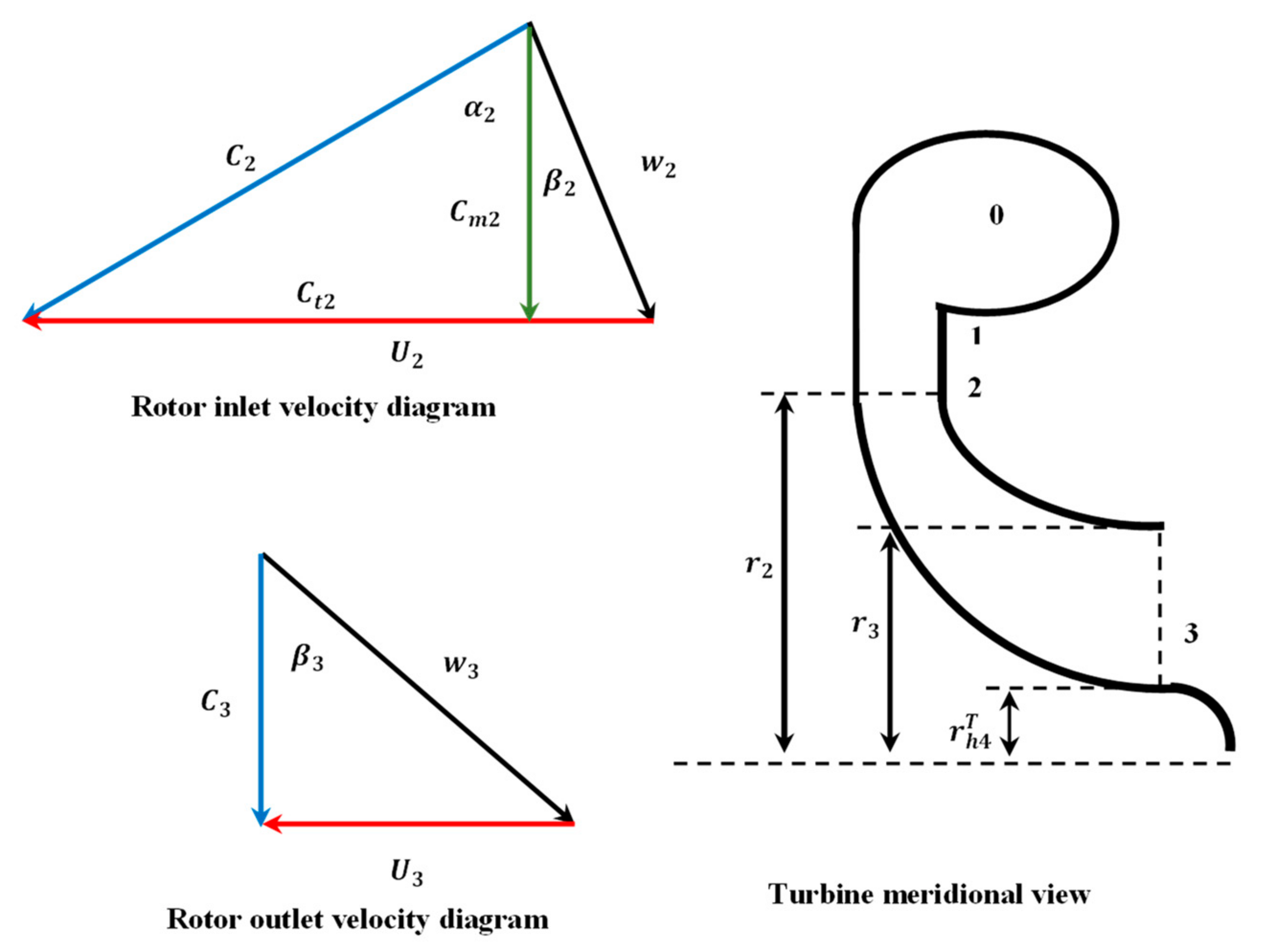
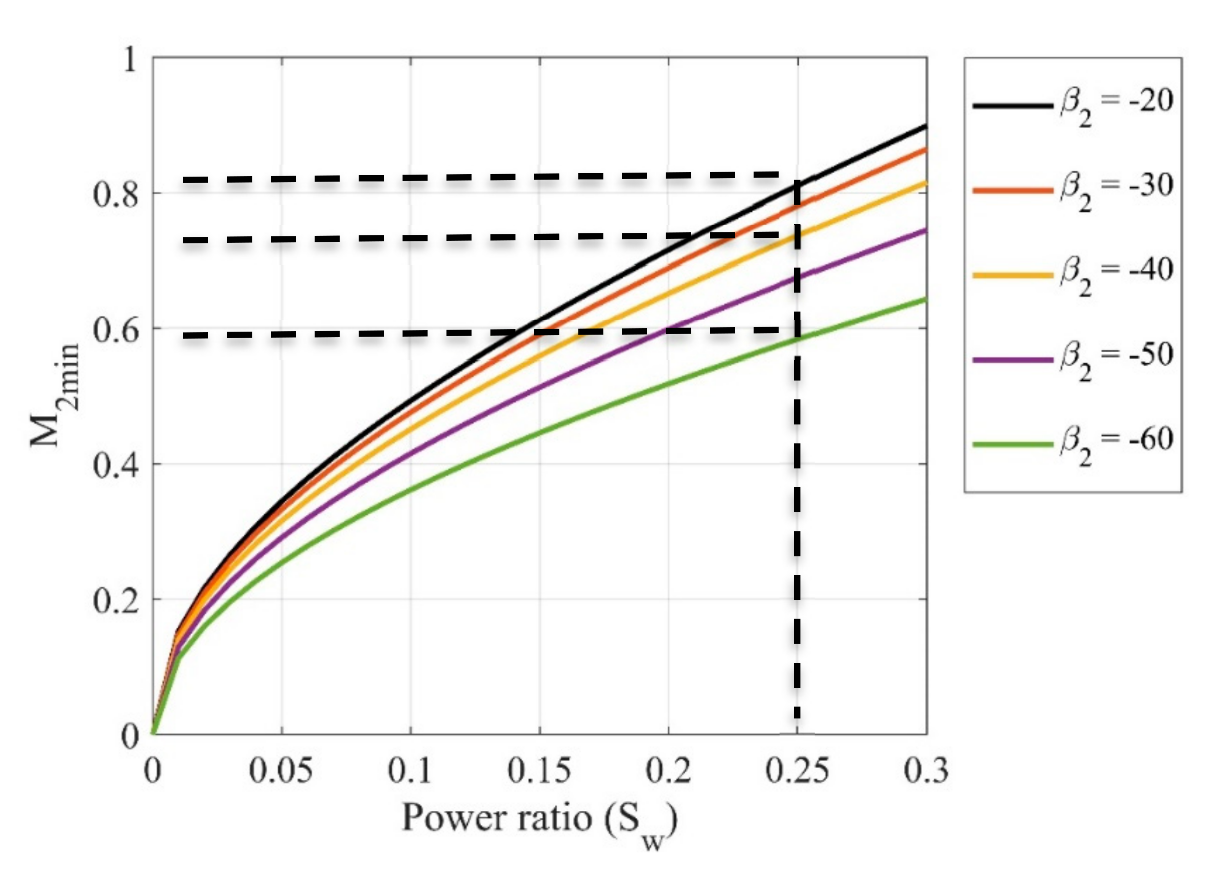
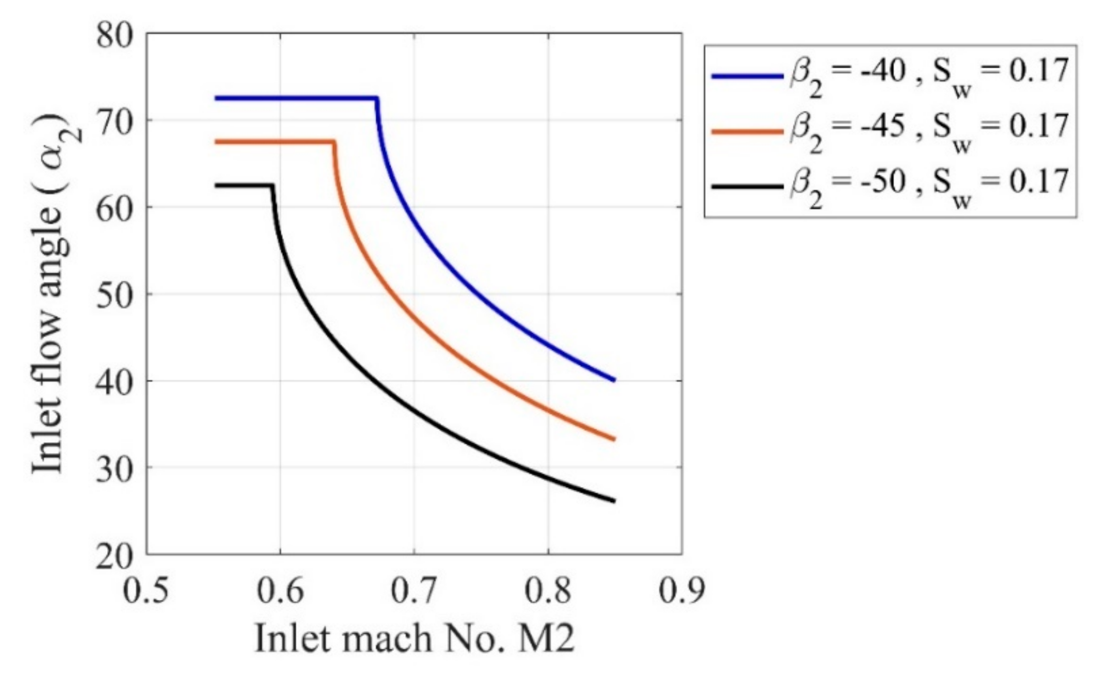
2.1.1. Design of the Rotor Inlet
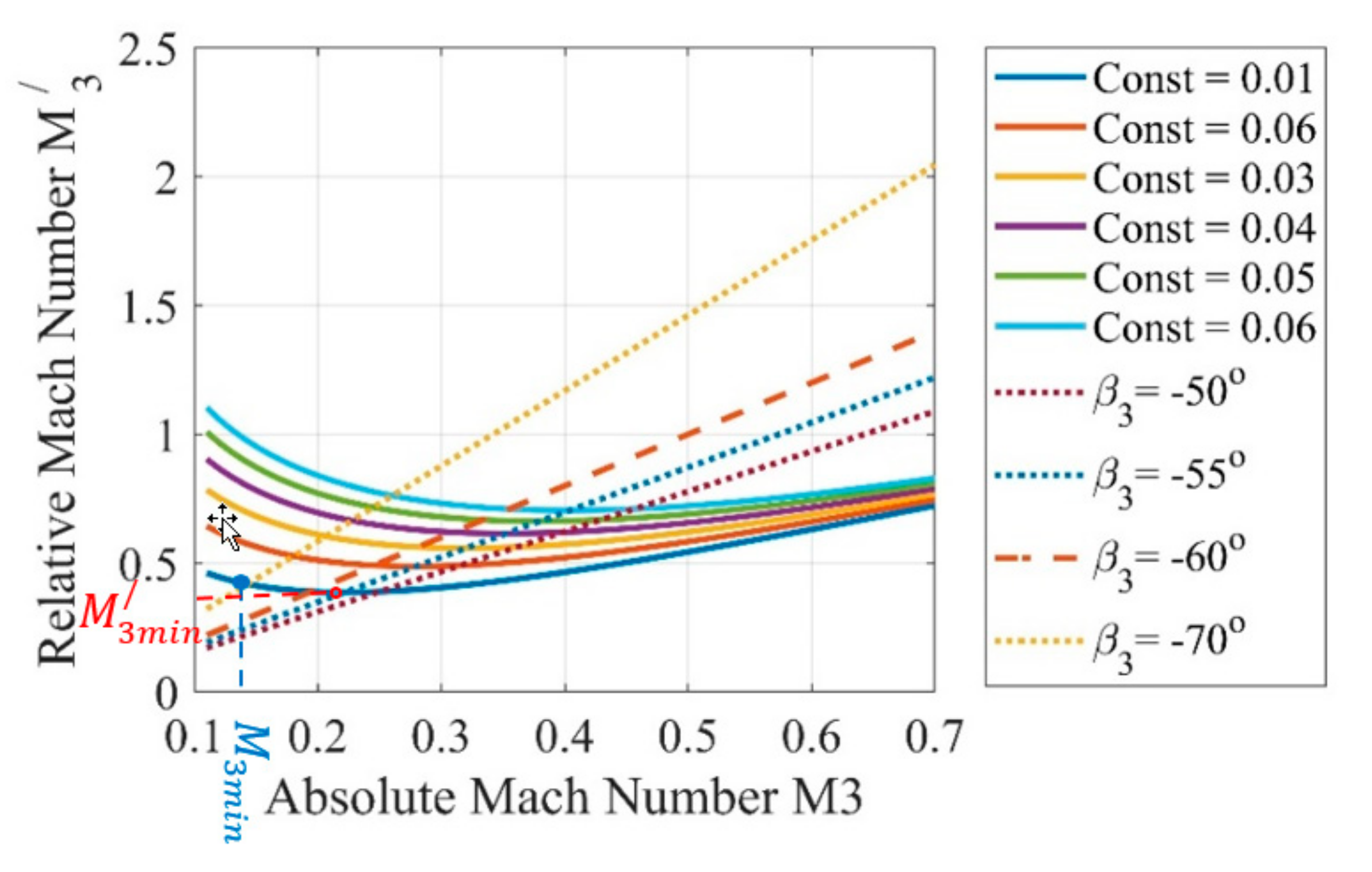
2.1.2. Design of Rotor Outlet
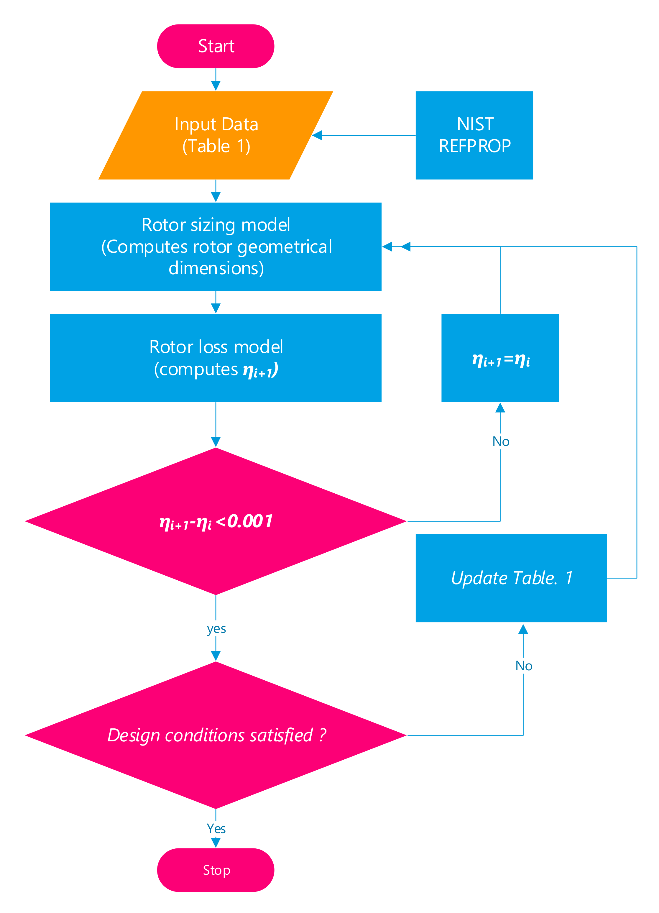
2.2. Meanline Design of the Turbine
2.2.1. Rotor Loss Model
2.2.2. Friction Losses
2.2.3. Tip Clearance Losses
2.2.4. Exit and Secondary Losses
3. Response Surface Optimization
4. Computation Model
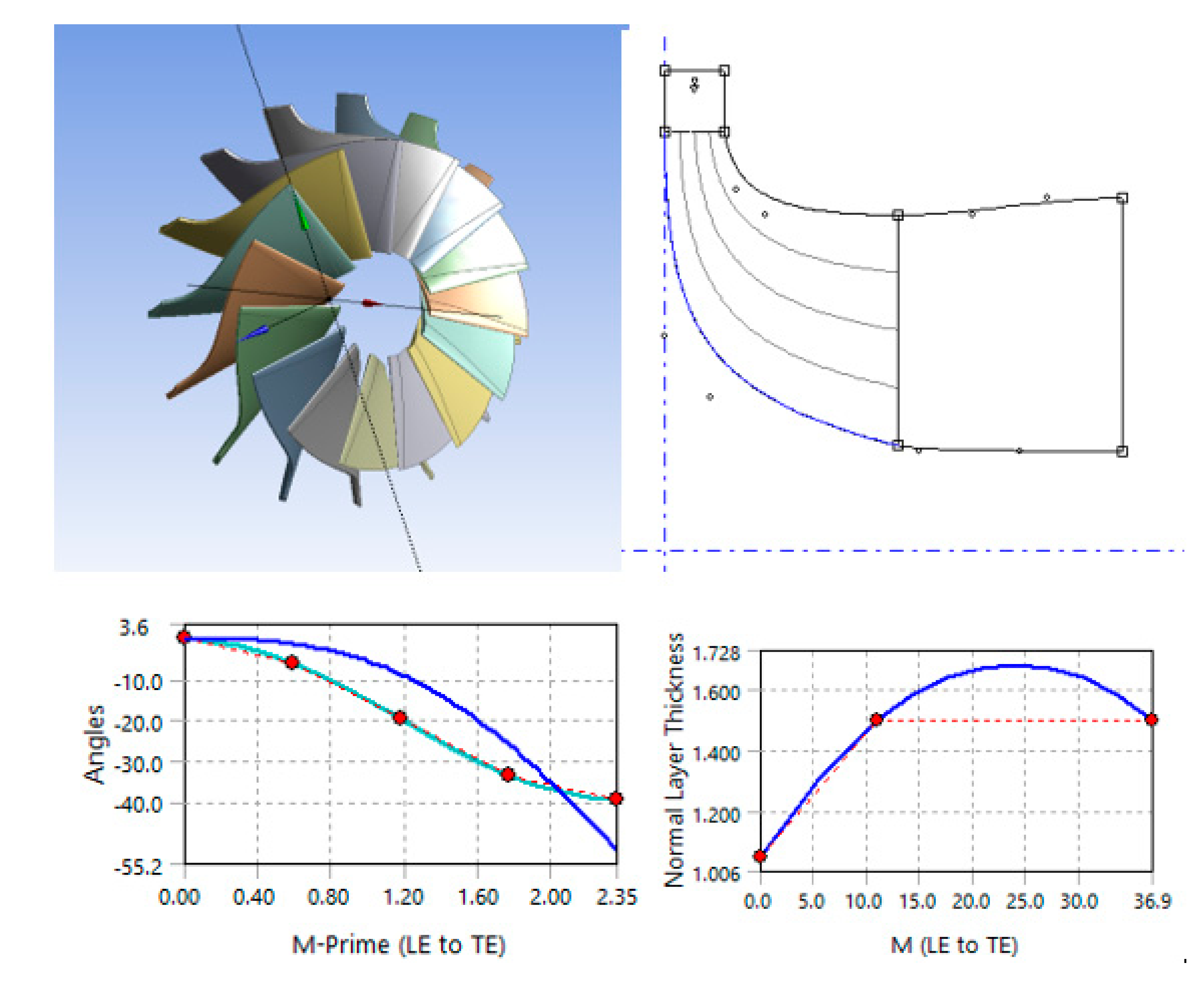
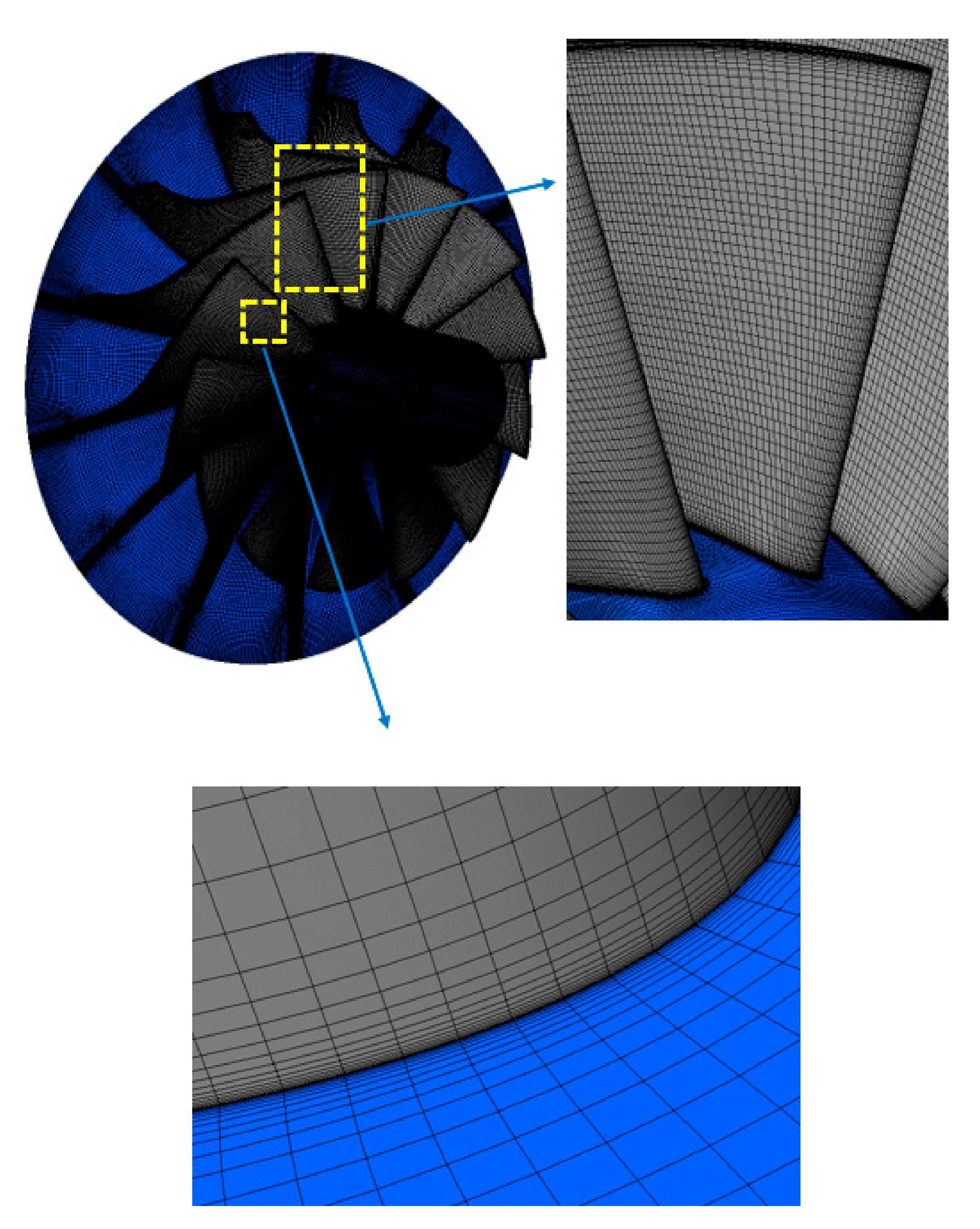
4.1. Turbine Geometry/Meshing
4.2. Computation Method and Boundary Equations
5. Results
5.1. Rotor Optimization
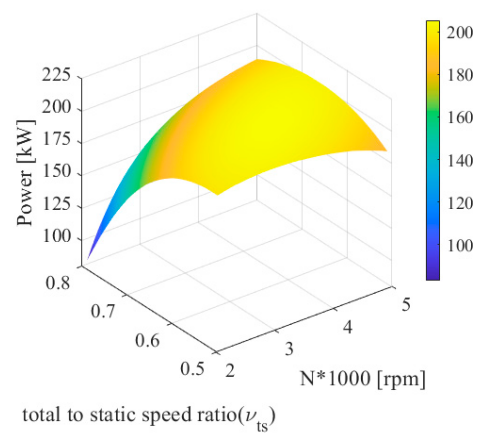
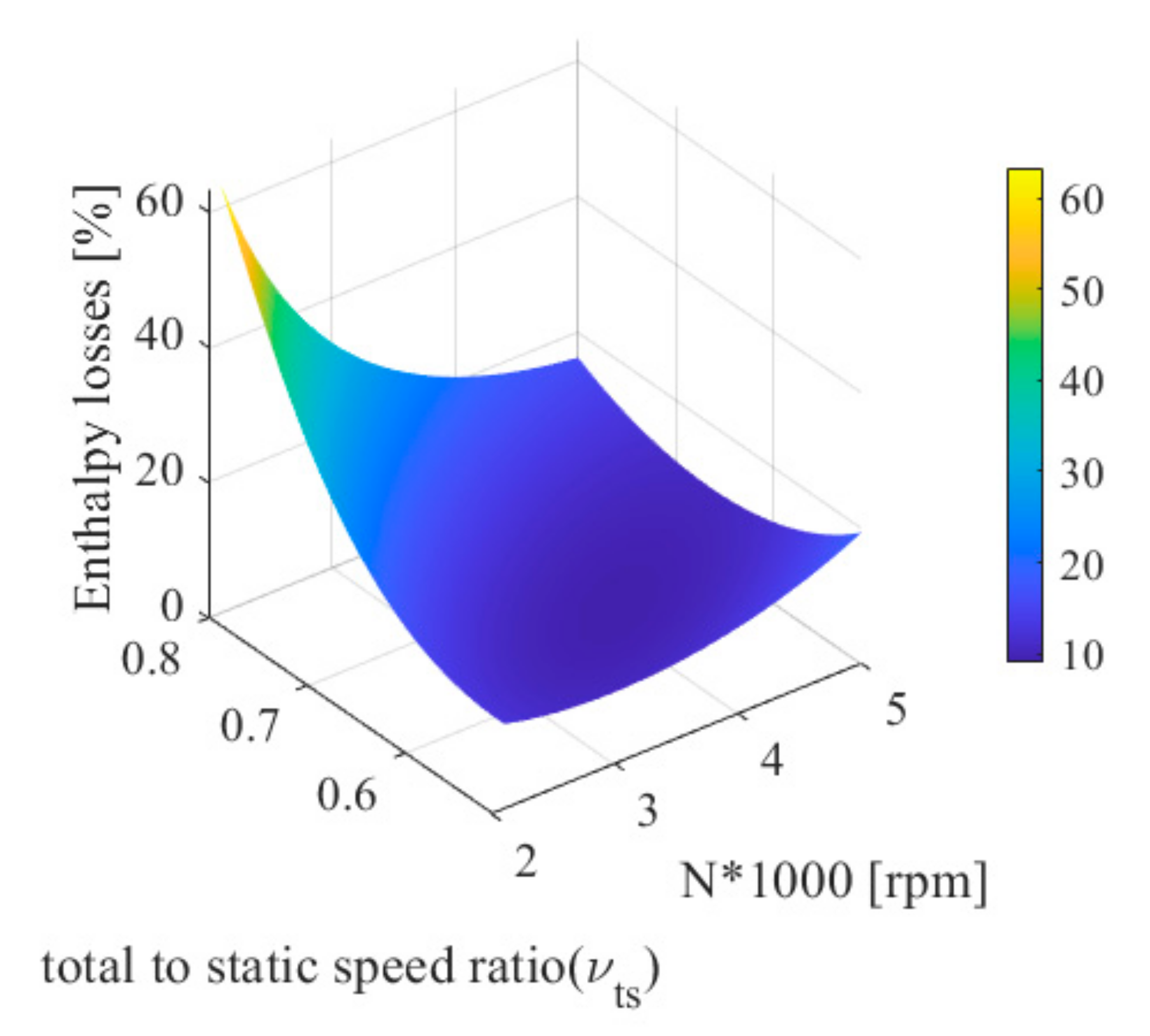
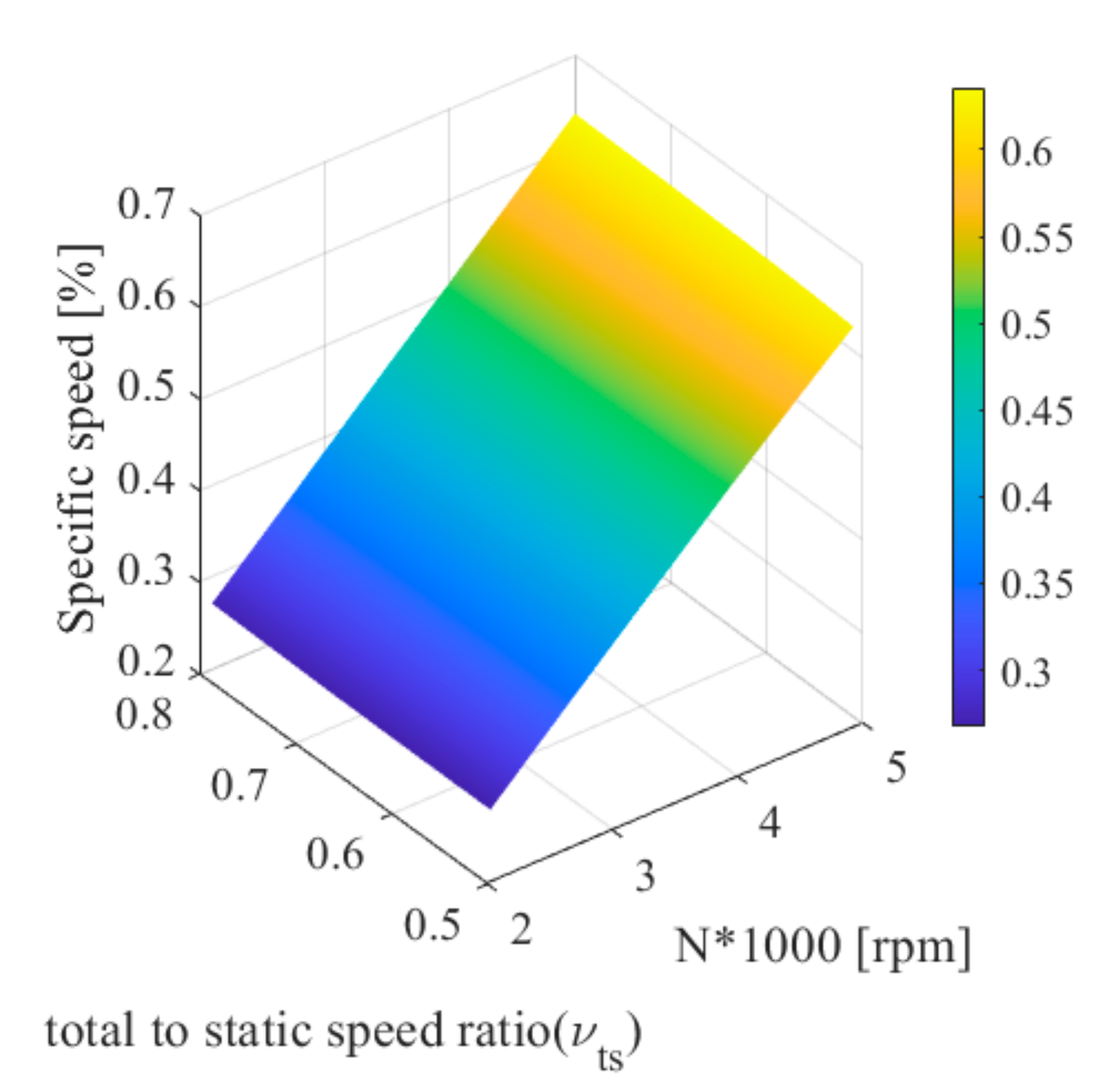
5.1.1. Response Surfaces Bounded by and Rotor Rotational Speed
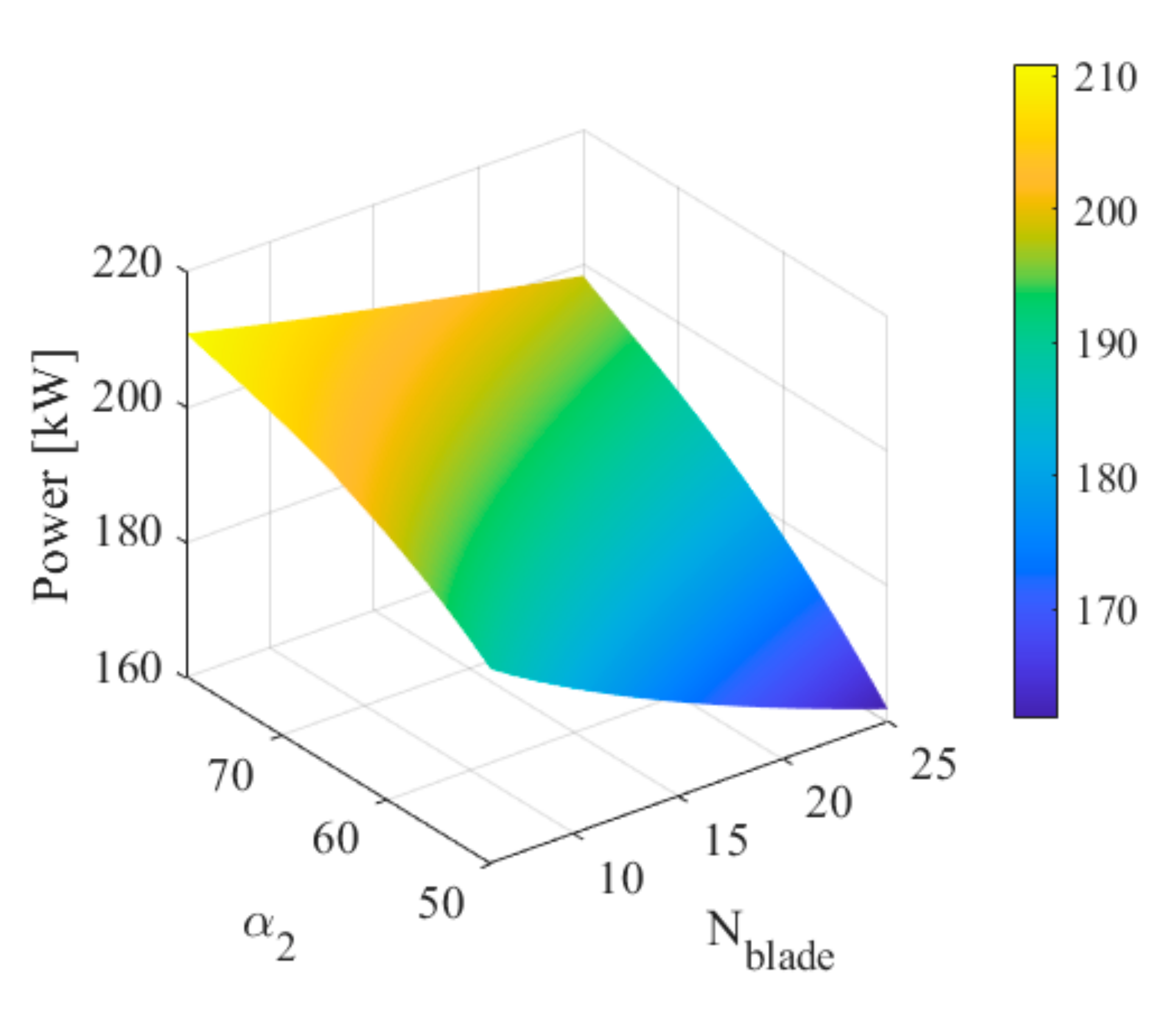
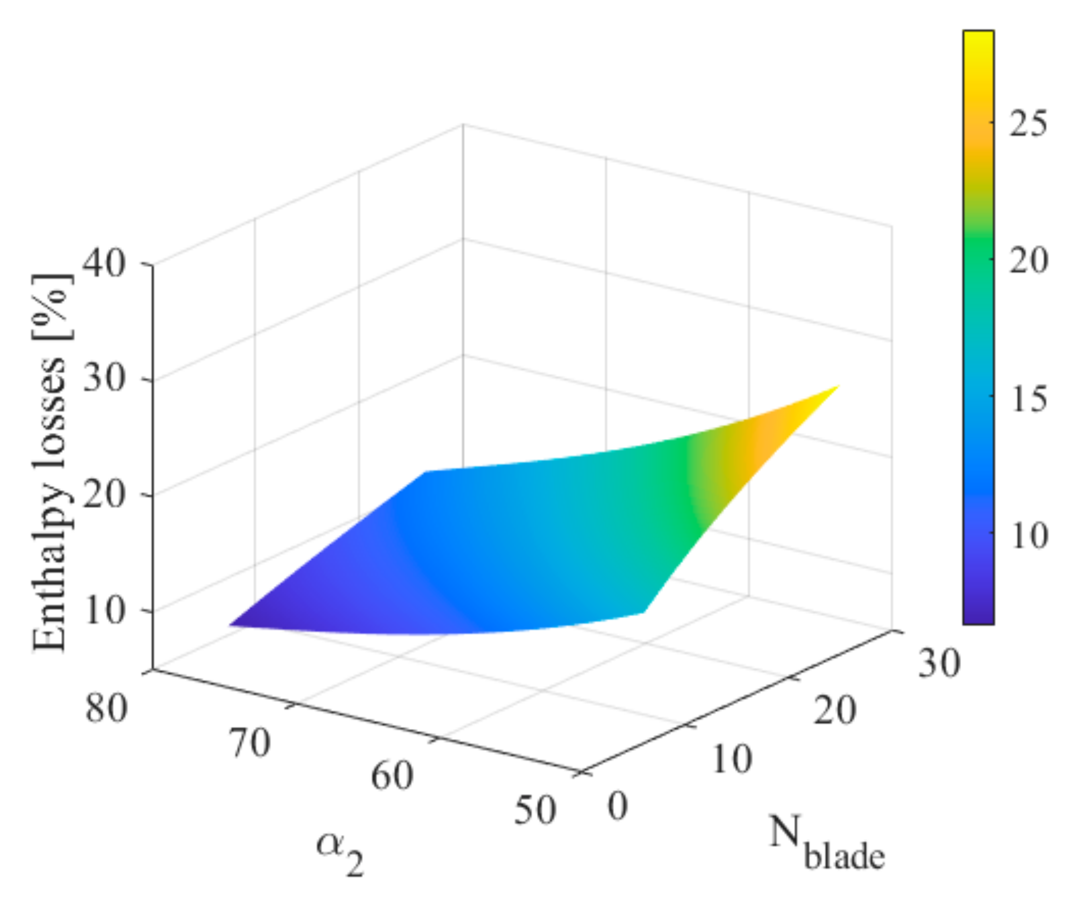
5.1.2. Response Surfaces Bounded by and Number of Blades
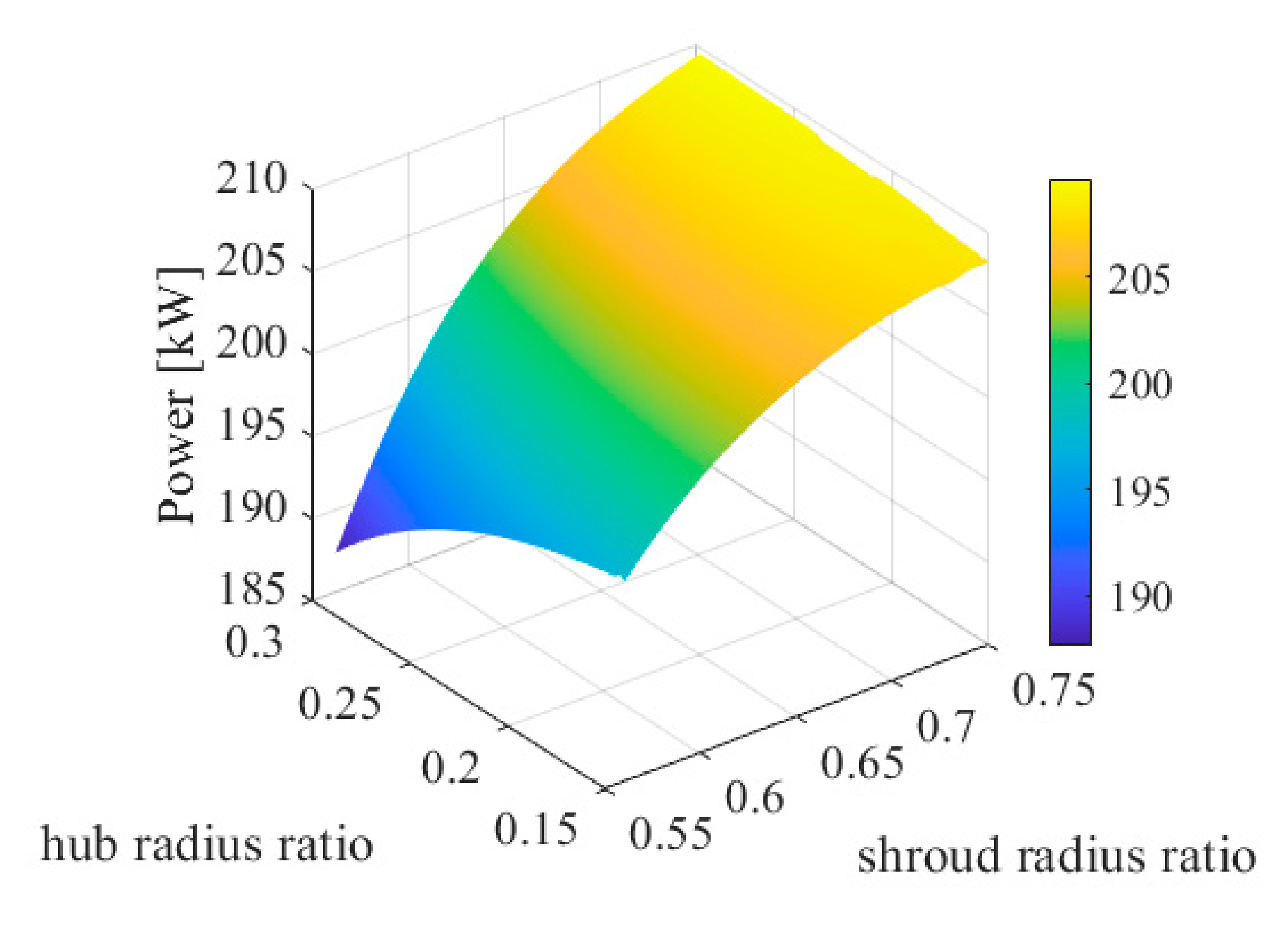
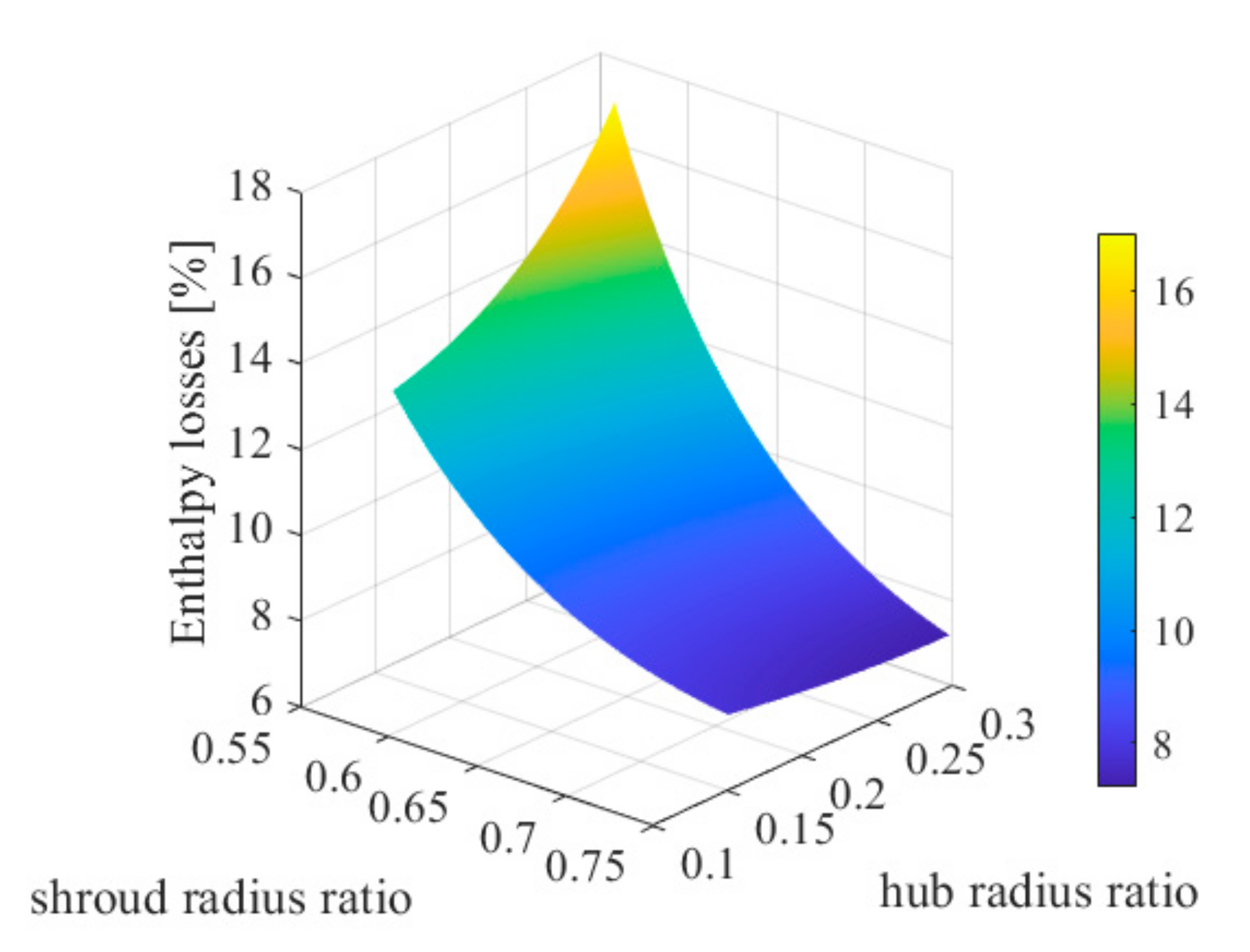
5.1.3. Response Surfaces Bounded by Hub Radius Ratio and Shroud Radius Ratio
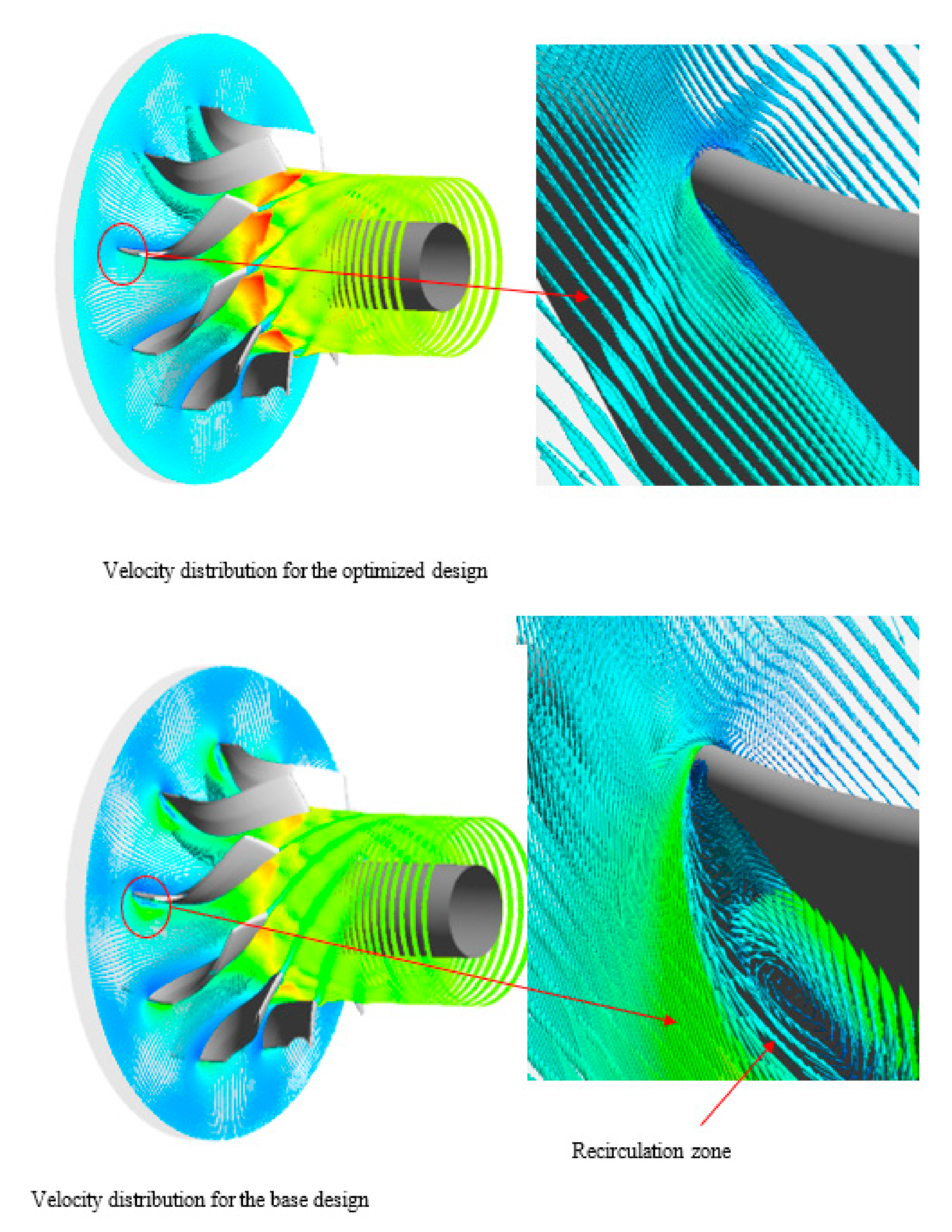
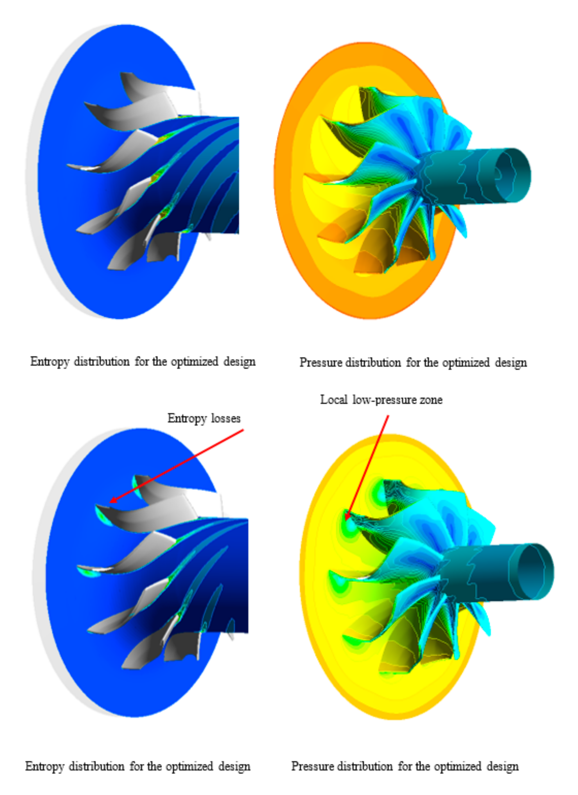
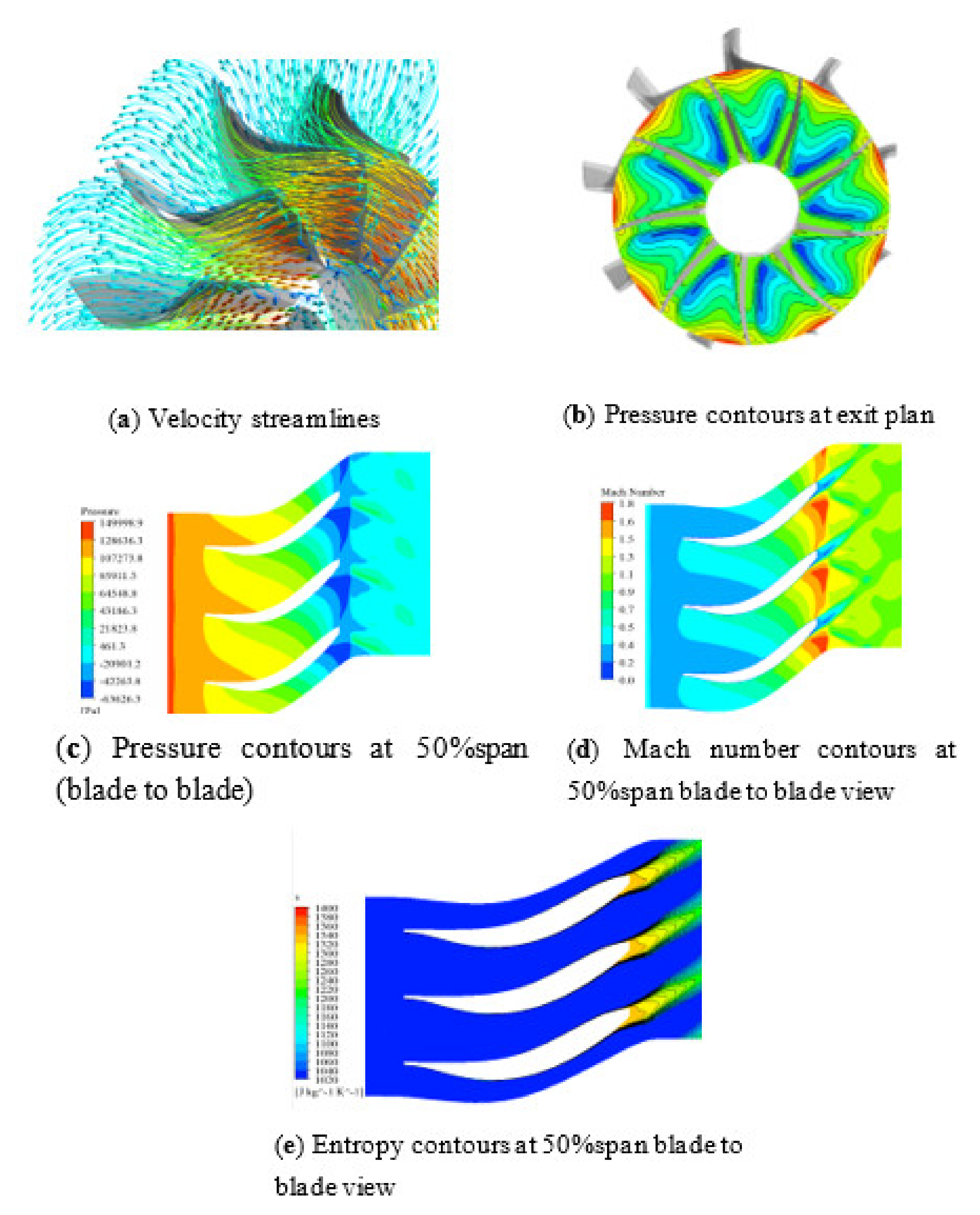
5.1.4. Comparison of Meanline Design/Optimized Design with CFD Results
6. Conclusions
- For an accurate design calculation process, the accurate prediction of thermo—physical properties is crucial. For the current design process, MATLAB code was linked with NIST’s REFPROP for the accurate provision of the properties. That is a distinct feature of the current study that has been ignored in similar studies found in the literature.
- It has been shown that a better meanline design based on the best design practices can significantly reduce the computation time and resources in the design and optimization of the turbine.
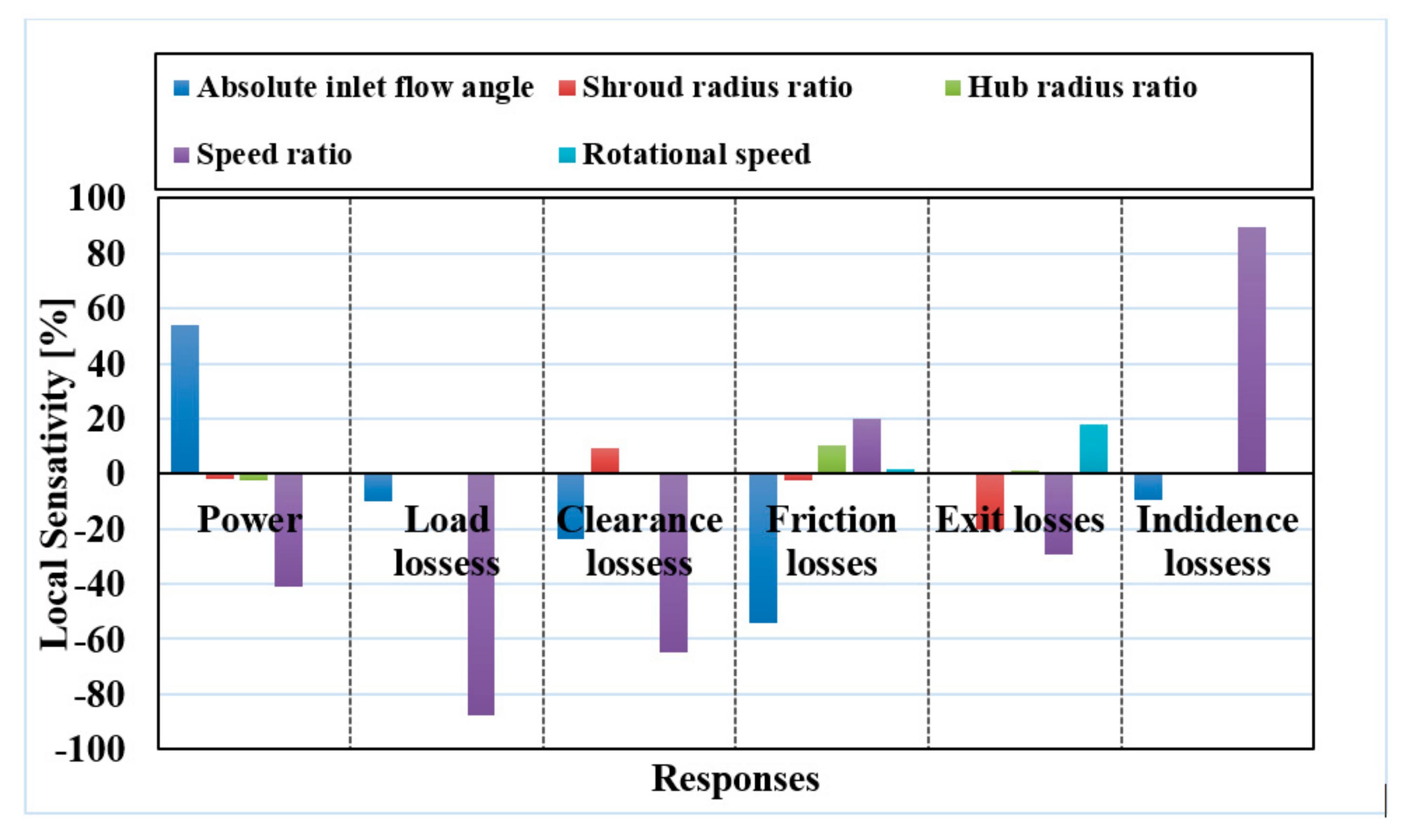
- The design optimization process is based on minimizing the losses, thus maximizing power and efficiency. For the current study, an improvement of 4.7% in power and 4.2% in efficiency is achieved through the optimization process.
- The maximum deviation in the meanline and CFD calculation was found for the output power of the turbine, which is 5.42%.
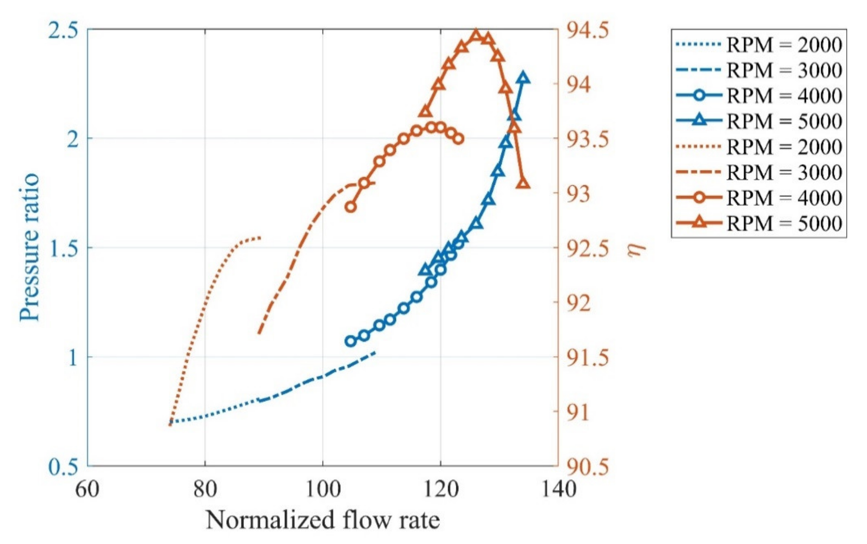
- Reported off-design results add to an additional validation toward the effectiveness of the procedure suggested for the design and estimation of a radial turbine.
- Response surface methodology (RSM) integrated with the 3D-RANS calculation is an effective, reliable, and robust method of the design and optimization of turbomachinery.
Author Contributions
Funding
Conflicts of Interest
Nomenclature
| speed of sound | |
| width of the blade | |
| absolute speed | |
| specific heat capacity ] | |
| rotor tip clearance (axial) ] | |
| rotor tip clearance (radial) ] | |
| hydraulic diameter | |
| friction factor | |
| specific enthalpy | |
| hydraulic length | |
| mass flow rate | |
| Mach number | |
| rotational speed [rpm] | |
| specific speed | |
| pressure | |
| Flow rate | |
| Radius [m] | |
| Reynolds number | |
| power ratio | |
| blade thickness | |
| temperature | |
| tangential speed of rotor | |
| velocity | |
| relative speed | |
| power | |
| rotor length |
Greek Symbols
| velocity angle (absolute) [degree] | |
| velocity angle (relative) [degree] | |
| efficiency | |
| dynamic viscosity | |
| density | |
| angular speed | |
| specific heat capacity ratio |
Sub and Super Scripts
| / | relative component |
| 0 | stagnation |
| 1 | nozzle inlet |
| 2 | rotor inlet |
| 3 | rotor exit |
| blade | |
| cycle | |
| compressor | |
| hub | |
| maximum value | |
| minimum value | |
| Shroud, isentropic | |
| turbine | |
| tangential direction |
References
- Kim, D.-Y.; Kim, Y.-T. Preliminary design and performance analysis of a radial inflow turbine for organic Rankine cycles. Appl. Therm. Eng. 2017, 120, 549–559. [Google Scholar] [CrossRef]
- Wang, T.; Ding, L.; Gu, C.; Yang, B. Performance analysis and improvement for CC-OTEC system. J. Mech. Sci. Technol. 2008, 22, 1977–1983. [Google Scholar] [CrossRef]
- Bharathan, D. Staging Rankine Cycles Using Ammonia for OTEC Power Production; National Renewable Energy Laboratory: Golden, CO, USA, 2009.
- Goto, S.; Motoshima, Y.; Sugi, T.; Yasunaga, T.; Ikegami, Y.; Nakamura, M. Construction of simulation model for OTEC plant using Uehara cycle. Electr. Eng. Jpn. 2011, 176, 1–13. [Google Scholar] [CrossRef]
- Yang, M.-H.; Yeh, R.-H. Analysis of optimization in an OTEC plant using organic Rankine cycle. Renew. Energy 2014, 68, 25–34. [Google Scholar] [CrossRef]
- Kim, A.S.; Kim, H.-J.; Lee, H.-S.; Cha, S. Dual-use open cycle ocean thermal energy conversion (OC-OTEC) using multiple condensers for adjustable power generation and seawater desalination. Renew. Energy 2016, 85, 344–358. [Google Scholar] [CrossRef]
- Mohd Idrus, N.H.; Musa, M.N.; Yahya, W.J.; Ithnin, A.M. Geo-ocean thermal energy conversion (GeOTEC) power cycle/plant. Renew. Energy 2017, 111, 372–380. [Google Scholar] [CrossRef]
- Goto, S.; Matsuda, Y.; Sugi, T.; Morisaki, T.; Yasunaga, T.; Ikegami, Y.; Egashira, N. Web Application for OTEC Simulator Using Double-Stage Rankine Cycle. IFAC Pap. Online 2017, 50, 121–128. [Google Scholar] [CrossRef]
- Brun, K.; Friedman, P.; Dennis, R. Fundamentals and Applications of Supercritical Carbon Dioxide (sCO2) Based Power Cycles; Elsevier: Amsterdam, The Netherlands, 2017. [Google Scholar]
- Li, Y.; Ren, X. Investigation of the organic Rankine cycle (ORC) system and the radial-inflow turbine design. Appl. Therm. Eng. 2016, 96, 547–554. [Google Scholar] [CrossRef]
- Zhai, L.; Xu, G.; Wen, J.; Quan, Y.; Fu, J.; Wu, H.; Li, T. An improved modeling for low-grade organic Rankine cycle coupled with optimization design of radial-inflow turbine. Energy Convers. Manag. 2017, 153, 60–70. [Google Scholar] [CrossRef]
- Mounier, V.; Olmedo, L.E.; Schiffmann, J. Small scale radial inflow turbine performance and pre-design maps for Organic Rankine Cycles. Energy 2018, 143, 1072–1084. [Google Scholar] [CrossRef]
- Saeed, M.; Khatoon, S.; Kim, M.-H. Design optimization and performance analysis of a supercritical carbon dioxide recompression Brayton cycle based on the detailed models of the cycle components. Energy Convers. Manag. 2019, 196, 242–260. [Google Scholar] [CrossRef]
- Saeed, M.; Kim, M. Analysis of a recompression supercritical carbon dioxide power cycle with an integrated turbine design/optimization algorithm. Energy 2018, 165, 93–111. [Google Scholar] [CrossRef]
- Zheng, Y.; Hu, D.; Cao, Y.; Dai, Y. Preliminary design and off-design performance analysis of an Organic Rankine Cycle radial-inflow turbine based on mathematic method and CFD method. Appl. Therm. Eng. 2017, 112, 25–37. [Google Scholar] [CrossRef]
- Kim, J.-S.; Kim, D.-Y. Preliminary Design and Off-Design Analysis of a Radial Outflow Turbine for Organic Rankine Cycles. Energies 2020, 13, 2118. [Google Scholar] [CrossRef]
- Lemmon, E.; McLinden, M.; Huber, M. NIST Reference Fluid Thermodynamic and Transport Properties Database: REFPROP, Version 9.1; NIST Standard Reference Database 23; NIST: Gaithersburg, MD, USA, 2013. [Google Scholar]
- ANSYS CFX-Pre User’s Guide Release 16.0; ANSYS: Canonsburg, PA, USA, 2015.
- Han, Z.; Fan, W.; Zhao, R. Improved thermodynamic design of organic radial-inflow turbine and ORC system thermal performance analysis. Energy Convers. Manag. 2017, 150, 259–268. [Google Scholar] [CrossRef]
- Aungier, R.H. Mean streamline aerodynamic performance analysis of centrifugal compressors. J. Turbomach. 1995, 117, 360. [Google Scholar] [CrossRef]
- Aungier, R.H. Turbine Aerodynamics: Axial-Flow and Radial-Flow Turbine Design and Analysis; ASME: New York, NY, USA, 2006. [Google Scholar]
- Moustapha, H. Axial and Radial Turbines, 1st ed.; Concepts NREC: White River Junction, VT, USA, 2003. [Google Scholar]
- Bradley, N.; Cheng, A.Y.; Guan, Z.; Vrajitoru, D. The Response Surface Methodology; Indiana University of South Bend: South Bend, India, 2007. [Google Scholar]
- Mohammed, B.S.; Hossain, K.M.A.; Ting, J.; Swee, E.; Wong, G.; Abdullahi, M. Properties of crumb rubber hollow concrete block. J. Clean. Prod. 2012, 23, 57–67. [Google Scholar] [CrossRef]
- Mohammed, B.S.; Khed, V.C.; Nuruddin, M.F. Rubbercrete mixture optimization using response surface methodology. J. Clean. Prod. 2018, 171, 1605–1621. [Google Scholar] [CrossRef]
- Madsen, J.I.; Shyy, W.; Haftka, R.T. Response surface techniques for diffuser shape optimization. AIAA J. 2000, 38, 1512–1518. [Google Scholar] [CrossRef]
- Ahn, J.; Kim, H.-J.; Lee, D.-H.; Rho, O.-H. Response surface method for airfoil design in transonic flow. J. Aircr. 2001, 38, 231–238. [Google Scholar] [CrossRef]
- Ha, S.T.; Ngo, L.C.; Saeed, M.; Jeon, B.J.; Choi, H. A comparative study between partitioned and monolithic methods for the problems with 3D fluid-structure interaction of blood vessels. J. Mech. Sci. Technol. 2017, 31, 281–287. [Google Scholar] [CrossRef]


| Turbine Inlet Temperature | ||
|---|---|---|
| Turbine inlet total pressure | ||
| Turbine outlet static pressure | ||
| Mass flow rate | ||
| Isentropic specific power | ||
| Specific speed | ||
| Total to static velocity ratio | ||
| Total to static efficiency first iteration | ||
| Shrouds exit to rotor inlet radius | ||
| Hub exit to rotor inlet radius | ||
| Number of rotor blades | ||
| Rotor inlet absolute velocity angle |
| Input Design Variable for the Optimization Procedure | Lower Limit | Upper Limit | |
|---|---|---|---|
| Speed ratio () | 0.8 | ||
| Absolute flow angle at rotor inlet () [degree] | 80 | ||
| Rotational speed | 2000 | 5000 | |
| () | 0.80 | ||
| ( | 0.30 |
| S.No. | |||||
|---|---|---|---|---|---|
| 1 | 65.00 | 0.65 | 0.22 | 3500 | 0.68 |
| 2 | 50.00 | 0.65 | 0.22 | 3500 | 0.68 |
| 3 | 57.50 | 0.65 | 0.22 | 3500 | 0.68 |
| 4 | 80.00 | 0.65 | 0.22 | 3500 | 0.68 |
| 5 | 72.50 | 0.65 | 0.22 | 3500 | 0.68 |
| 6 | 65.00 | 0.55 | 0.22 | 3500 | 0.68 |
| 7 | 65.00 | 0.60 | 0.22 | 3500 | 0.68 |
| 8 | 65.00 | 0.75 | 0.22 | 3500 | 0.68 |
| 9 | 65.00 | 0.70 | 0.22 | 3500 | 0.68 |
| 10 | 65.00 | 0.65 | 0.15 | 3500 | 0.68 |
| 11 | 65.00 | 0.65 | 0.19 | 3500 | 0.68 |
| 12 | 65.00 | 0.65 | 0.30 | 3500 | 0.68 |
| 13 | 65.00 | 0.65 | 0.26 | 3500 | 0.68 |
| 14 | 65.00 | 0.65 | 0.22 | 2000 | 0.68 |
| 15 | 65.00 | 0.65 | 0.22 | 2750 | 0.68 |
| 16 | 65.00 | 0.65 | 0.22 | 5000 | 0.68 |
| 17 | 65.00 | 0.65 | 0.22 | 4250 | 0.68 |
| 18 | 65.00 | 0.65 | 0.22 | 3500 | 0.55 |
| 19 | 65.00 | 0.65 | 0.22 | 3500 | 0.61 |
| 20 | 65.00 | 0.65 | 0.22 | 3500 | 0.80 |
| 21 | 65.00 | 0.65 | 0.22 | 3500 | 0.74 |
| 22 | 50.00 | 0.55 | 0.15 | 2000 | 0.80 |
| 23 | 57.50 | 0.60 | 0.19 | 2750 | 0.74 |
| 24 | 80.00 | 0.55 | 0.15 | 2000 | 0.55 |
| 25 | 72.50 | 0.60 | 0.19 | 2750 | 0.61 |
| 26 | 50.00 | 0.75 | 0.15 | 2000 | 0.55 |
| 27 | 57.50 | 0.70 | 0.19 | 2750 | 0.61 |
| 28 | 80.00 | 0.75 | 0.15 | 2000 | 0.80 |
| 29 | 72.50 | 0.70 | 0.19 | 2750 | 0.74 |
| 30 | 50.00 | 0.55 | 0.30 | 2000 | 0.55 |
| 31 | 57.50 | 0.60 | 0.26 | 2750 | 0.61 |
| 32 | 80.00 | 0.55 | 0.30 | 2000 | 0.80 |
| 33 | 72.50 | 0.60 | 0.26 | 2750 | 0.74 |
| 34 | 50.00 | 0.75 | 0.30 | 2000 | 0.80 |
| 35 | 57.50 | 0.70 | 0.26 | 2750 | 0.74 |
| 36 | 80.00 | 0.75 | 0.30 | 2000 | 0.55 |
| 37 | 72.50 | 0.70 | 0.26 | 2750 | 0.61 |
| 38 | 50.00 | 0.55 | 0.15 | 5000 | 0.55 |
| 39 | 57.50 | 0.60 | 0.19 | 4250 | 0.61 |
| 40 | 80.00 | 0.55 | 0.15 | 5000 | 0.80 |
| 41 | 72.50 | 0.60 | 0.19 | 4250 | 0.74 |
| 42 | 50.00 | 0.75 | 0.15 | 5000 | 0.80 |
| 43 | 57.50 | 0.70 | 0.19 | 4250 | 0.74 |
| 44 | 80.00 | 0.75 | 0.15 | 5000 | 0.55 |
| 45 | 72.50 | 0.70 | 0.19 | 4250 | 0.61 |
| 46 | 50.00 | 0.55 | 0.30 | 5000 | 0.80 |
| 47 | 57.50 | 0.60 | 0.26 | 4250 | 0.74 |
| 48 | 80.00 | 0.55 | 0.30 | 5000 | 0.55 |
| 49 | 72.50 | 0.60 | 0.26 | 4250 | 0.61 |
| 50 | 50.00 | 0.75 | 0.30 | 5000 | 0.55 |
| Turbine’s Geometry and Performance Parameters | Values (Baseline Design) | Values (Optimized Design) | Difference [%] |
|---|---|---|---|
| () | 0.8 | 0.69 | −13.75 |
| () [degree] | 65 | 82 | 26.15 |
| () | 0.18 | 0.25 | 38.89 |
| ( | 0.65 | 0.79 | 21.54 |
| Rotational speed [RPM] | 5000 | 3800 | −24.00 |
| () | 11.184 | 11.184 | 0.00 |
| Power [kW] | 194.6 | 204.22 | 4.94 |
| Total to static efficiency [%] | 87.01 | 91.3 | 4.93 |
| Parameter | Meanline Design Calculation | CFD | Deviation [%] |
|---|---|---|---|
| Total to total pressure ratio | 1.439 | 1.411 | 1.94 |
| Total to static pressure ratio | 1.465 | 1.465 | 0 |
| Mass flow rate | 20 | 20.61 | 3.05 |
| Total to static efficiency ( | 91.3 | 93.4 | 2.30 |
| Power output | 204.22 | 215.29 | 5.42 |
Publisher’s Note: MDPI stays neutral with regard to jurisdictional claims in published maps and institutional affiliations. |
© 2020 by the authors. Licensee MDPI, Basel, Switzerland. This article is an open access article distributed under the terms and conditions of the Creative Commons Attribution (CC BY) license (http://creativecommons.org/licenses/by/4.0/).
Share and Cite
Alawadhi, K.; Alhouli, Y.; Ashour, A.; Alfalah, A. Design and Optimization of a Radial Turbine to Be Used in a Rankine Cycle Operating with an OTEC System. J. Mar. Sci. Eng. 2020, 8, 855. https://doi.org/10.3390/jmse8110855
Alawadhi K, Alhouli Y, Ashour A, Alfalah A. Design and Optimization of a Radial Turbine to Be Used in a Rankine Cycle Operating with an OTEC System. Journal of Marine Science and Engineering. 2020; 8(11):855. https://doi.org/10.3390/jmse8110855
Chicago/Turabian StyleAlawadhi, Khaled, Yousef Alhouli, Ali Ashour, and Abdullah Alfalah. 2020. "Design and Optimization of a Radial Turbine to Be Used in a Rankine Cycle Operating with an OTEC System" Journal of Marine Science and Engineering 8, no. 11: 855. https://doi.org/10.3390/jmse8110855
APA StyleAlawadhi, K., Alhouli, Y., Ashour, A., & Alfalah, A. (2020). Design and Optimization of a Radial Turbine to Be Used in a Rankine Cycle Operating with an OTEC System. Journal of Marine Science and Engineering, 8(11), 855. https://doi.org/10.3390/jmse8110855