Derivation of Engineering Design Criteria for Flow Field Around Intake Structure: A Numerical Simulation Study

Abstract

The primary environmental impact caused by seawater intake operation is marine life impingement resulting from the intake velocity. Environmental Protection Agency (EPA) of United State has regulated the use of velocity cap fitted at intake structures to reduce the marine life impingement. The engineering design parameters of velocity cap has not been well explored to date. This study has been set to determine the fundamental relationships between intake velocity and design parameters of velocity cap, using computational fluid dynamic (CFD) model. A set of engineering design criteria for velocity cap design are derived. The numerical evidence yielded in this study show that the velocity cap should be designed with vertical opening (H_vc) and horizontal shelf (ℓ_vc). The recommended intake opening ratio (O_r) shall be 0.36 V_r^−0.31, where O_r = H_vc/ℓ_vc and V_r =V₀/V_pipe. V_o is the velocity at the intake window and V_pipe is the suction velocity at the intake pipe. The volume ratio (ω_r) between the velocity cap (ω_vc) and intake tower (ω_IT) is recommended at 0.11 V_r^−1.23. The positive outlooks that yielded from this study can be served as a design reference for velocity cap to mitigate the detrimental impacts from the existing intake structure.

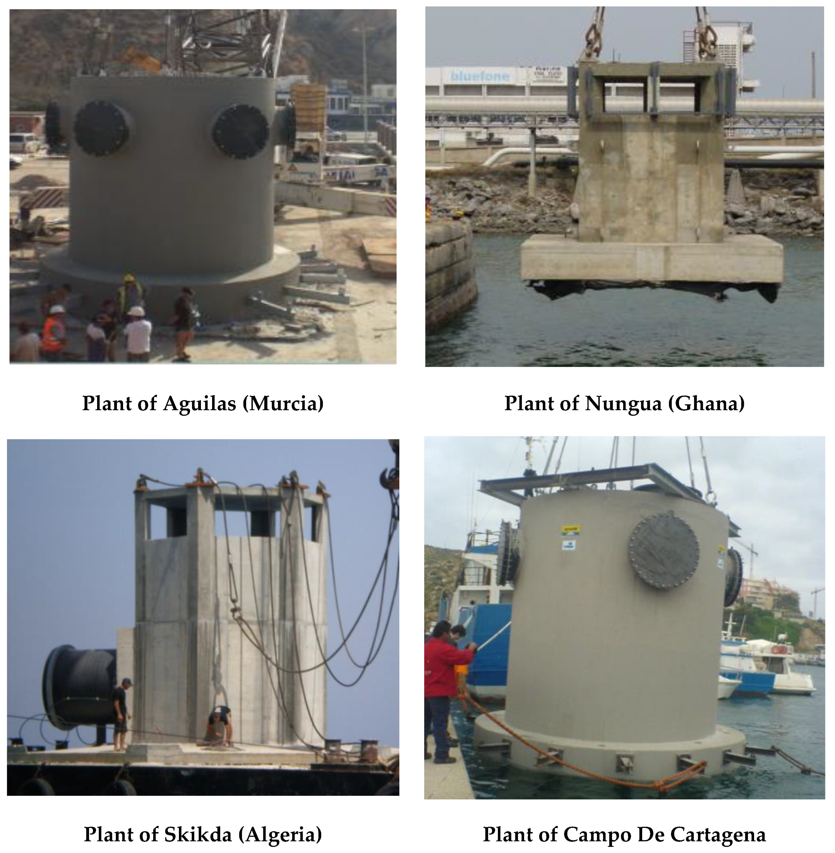
1. Introduction

Seawater intake structure are widely used by most coastal plants. A seawater intake structure usually made of reinforced concrete supporting the inlet of the withdrawal pipe. Figure 1 shows the photo examples of existing intake structures at Plant of Aguilas, Plant of Nungua, Plant of Skikda, and Plant of Campo De Cartagena [1]. Most of the intake towers are circular in shape with diameter ranging between 4.7 and 5.3 m. The intake tower height is between 5 and 7 m with intake rate between 1 and 7 m³/s. However, depending on the intake rate, the diameter of the intake tower can be ranging between 2 and 20 m [2]. The shape of the intake structure can be rectangular if it is designed to be in current, with shorter sides angled against the current. The marine life impingement and entrainment resulting from the intake operation is a major environment concern [3]. An optimum intake structural design should be operated in a way that minimizes marine impacts, particularly considering the impingement and entrainment of marine life. There are substantial literatures that points to increase intake mortality with increase intake velocities [4,5,6]. Even though fish are excellent swimmers, they can often be drawn in by vertical currents generated by intake velocity. The Environment Protection Agency of United State (USEPA) has suggested the use of velocity caps fitted at the intake structures to convert the water flow from vertical to horizontal [6]. The velocity cap, which is usually made of steel or concrete, is a simple modification to the unscreened intake in the open sea to draw water in horizontally. The used of velocity cap can reduce marine entrainment because fish are adapted to respond to horizontal current rather than vertical current fluctuations [7]. A change in horizontal flow pattern created by velocity cap will triggers an avoidance response mechanism in fish, which aids to reduce the marine life impingement [8]. The use of velocity cap can reduce 80% to 90% of the fish impingement at the intake entrance [9]. Based on this record of performance, USEPA has promulgated final ruling under the Clean Water Act to restrict the intake velocity to a maximum of 0.15 m/s and specify that seawater intake structures should be equipped with a velocity cap [10]. Electric Power Research Institute [11] has performed comprehensive literature reviews on the swimming capabilities of marine, freshwater, and estuarine fishes to determine the appropriateness of regulating 0.15 m/s as the maximum allowable intake velocity to preclude impingement impacts. They have concluded that intake velocity is an appropriate regulatory parameter, and it should be measured, preferably, as a vector parallel to the main water flow at the intake window. They highlighted that the 0.15 m/s intake velocity criterion can be useful to delineate where significant impingement impacts are unlikely to happen under common environmental conditions. Several federal and state agencies in US have also developed the intake velocity criteria to protect local populations of fish from being impinged at the intake window, and they generally proposed maximum allowable intake velocity of 0.15 m/s as an acceptable indicator of likely low occurrence of impingement problems at the intake structure [12,13].

Previous literature and sources of information reviewed did mentioned that velocity cap is one of the best technology available (BTA) and it shall result in a design intake velocity that less than or equal to 0.15 m/s. Figure 2 shows the schematic illustration of the flow in a capped intake structure. It is reasonable to speculate that the local flow conditions induced by the intake structure are the important fundamental to protect marine life from impingement mortality. However, to the author’s best knowledge, very little research work has been conducted in the area of engineering design criteria for velocity cap. Voutchkov (2018) [2] suggested the vertical opening of the velocity cap shall be between 1 and 3 m. Schuler and Larson (1975) [14] suggested that the horizontal distance of the velocity cap shall extend approximately 1.5 times the vertical opening. A key problem with many of these suggestions is that there are mostly based on “rules of thumb”, which have not been scientifically tested. This raises many questions about whether those intake design suggestions are suitable to be used for various structural configuration and intake rate. A variety of engineering properties, i.e., vertical opening and horizontal shelf of velocity cap are important contributory factors to influence the intake velocity. The literature review revealed that no single source of information or document precisely contained velocity cap design standards. Intake velocity requirement is significant and that this paper is essential for the understanding of fundamental relationships between the design parameters and intake velocity to derive engineering design criteria for environment protection.

A vast research has been undertaken to study the flow field around the coastal structure by using CFD models [15,16,17,18]. They have concluded that, with the advancement in numerical modelling tools, it is possible to analyze the fluid–structure interactions with numerical models. This paper presents the application of CFD model to simulate the flow field around an existing capped intake structure that located in Penang Strait of Malaysia. The existing capped intake structure was used to draw ambient seawater for power plant usage. The feasibility of the present numerical model was validated by comparing with the measured field values that obtained from secondary data source [19]. With proper data checking and data screening, field data has the advantage of being able to observe the outcome in a natural setting rather than in a contrived laboratory environment. Subsequently, the relationships between influencing design parameters and intake velocity are systematically analyzed and presented in SI unit. Finally, the engineering design criteria for intake structure is recommended.

2. Method

2.1. Numerical Model

The numerical investigation was undertaken using FLOW3D based on Reynolds’ Averaged Navier–Stokes (RANS) equations. The FLOW3D solver is structured upon the principle laws of mass, momentum and energy conservation, and the equations were solved using finite difference method. The central aim of any flow model is to provide projections of turbulent fluctuations on the flow quantities. This is commonly represented by including diffusion terms in the following mass and momentum transport equation:

$$V_F\frac{\partial \rho }{\partial t}+ \frac{\partial }{\partial x}\left(\rho u{A}_x\right)+R\frac{\partial }{\partial y}\left(\rho v{A}_y\right)+ \frac{\partial }{\partial z}\left(\rho w{A}_z\right)+\mathsf{\xi }\frac{\rho u{A}_x}{x}= R_{DIF }+ R_{SOR}$$

(1)

where $u, v$, and $w$ are fluid velocities in the Cartesian coordinate directions (x, y, z), A_x, A_y, and A_z are the fractional areas open to flow in the x, y, and z axis. V_F is the fractional volume open to flow, ρ is the fluid density, then R and ξ are coefficients that depend upon the choice of coordinate system. R_DIF and R_SOR are respectively the turbulent diffusion and mass source terms and are defined in Equations (2) and (3) below:

$$R_{DIF}= \frac{\partial }{\partial x}\left(v_{\rho }{A}_x\frac{\partial \rho }{\partial x}\right)+R\frac{\partial }{\partial y}\left(v_{\rho }{A}_{y}R\frac{\partial \rho }{\partial y}\right)+ \frac{\partial }{\partial z}\left(v_{\rho }{A}_z\frac{\partial \rho }{\partial z}\right)+\mathsf{\xi }\frac{v_{\rho }{A}_x}{x}\frac{\partial \rho }{\partial x}$$

(2)

$$\frac{\partial }{\partial x}\left(u{A}_x\right)+R\frac{\partial }{\partial y}\left(v{A}_y\right)+ \frac{\partial }{\partial z}\left(w{A}_z\right)+ \mathsf{\xi }\frac{u{A}_x}{x}= \frac{R_{SOR}}{\rho }$$

(3)

where υ_ρ = S_cμ/ρ, in which S_c is the turbulent Schmidt number and μ is the coefficient of momentum diffusion. The 3D equations of motion are solved with the following Navier–Stokes equations with some additional terms:

$$\begin{gathered} \frac{\partial u}{\partial t}+ \frac{1}{V_F} \left\{u{A}_x\frac{\partial u}{\partial x}+v{A}_{y}R\frac{\partial u}{\partial y}+w{A}_z\frac{\partial u}{\partial z}\right\}-\mathsf{\xi }\frac{A_y{v}^2}{x{V}_F} = -\frac{1}{\rho }\frac{\partial \rho }{\partial x}+ G_x+f_x- b_x- \frac{R_{SOR}}{\rho V_F}\left(u- u_w- \partial u_s\right) \\ \frac{\partial v}{\partial t}+ \frac{1}{V_F} \left\{u{A}_x\frac{\partial v}{\partial x}+v{A}_{y}R\frac{\partial v}{\partial y}+w{A}_z\frac{\partial v}{\partial z}\right\}+ \mathsf{\xi }\frac{A_{y}uv}{x{V}_F}= -\frac{1}{\rho }\frac{\partial \rho }{\partial y}+ G_y+f_y- b_y- \frac{R_{SOR}}{\rho V_F}\left(v- v_w- \partial v_s\right) \\ \frac{\partial w}{\partial t}+ \frac{1}{V_F} \left\{u{A}_x\frac{\partial w}{\partial x}+v{A}_{y}R\frac{\partial w}{\partial y}+w{A}_z\frac{\partial w}{\partial z}\right\}= -\frac{1}{\rho }\frac{\partial \rho }{\partial z}+ G_z+f_z- b_z- \frac{R_{SOR}}{\rho V_F}\left(w- w_w- \partial w_s\right) \end{gathered}$$

(4)

where t is the time, G_x, G_y and G_z are accelerations due to gravity, $f$_x, $f$_y, and $f$_z are viscous accelerations, and b_x, b_y, and b_z are the flow losses in porous media, $u_w$, $v_w$, and $w_w$ are velocity of the source component, $u_s$, $v_s$, and $w_s$ are velocity of the fluid at the surface of the source.

k-ε RNG turbulence model was suggested by Chie and Wahab (2019) [20] as the viscous model to simulate the flow kinematics around the intake structure. They tested the performance of four turbulence models, namely the standard k-epsilon (k-ε), k-ε renormalized group (RNG), k-omega (k–ω), and large eddy simulation (LES) models and concluded that k-ε RNG model can provide good accuracy and reduce the computational costs compared to the LES model. Furthermore, the k-ε RNG model [21] extend the capabilities of k-ε model to provide better coverage of low intensity turbulence flows and flow in areas with strong shear.

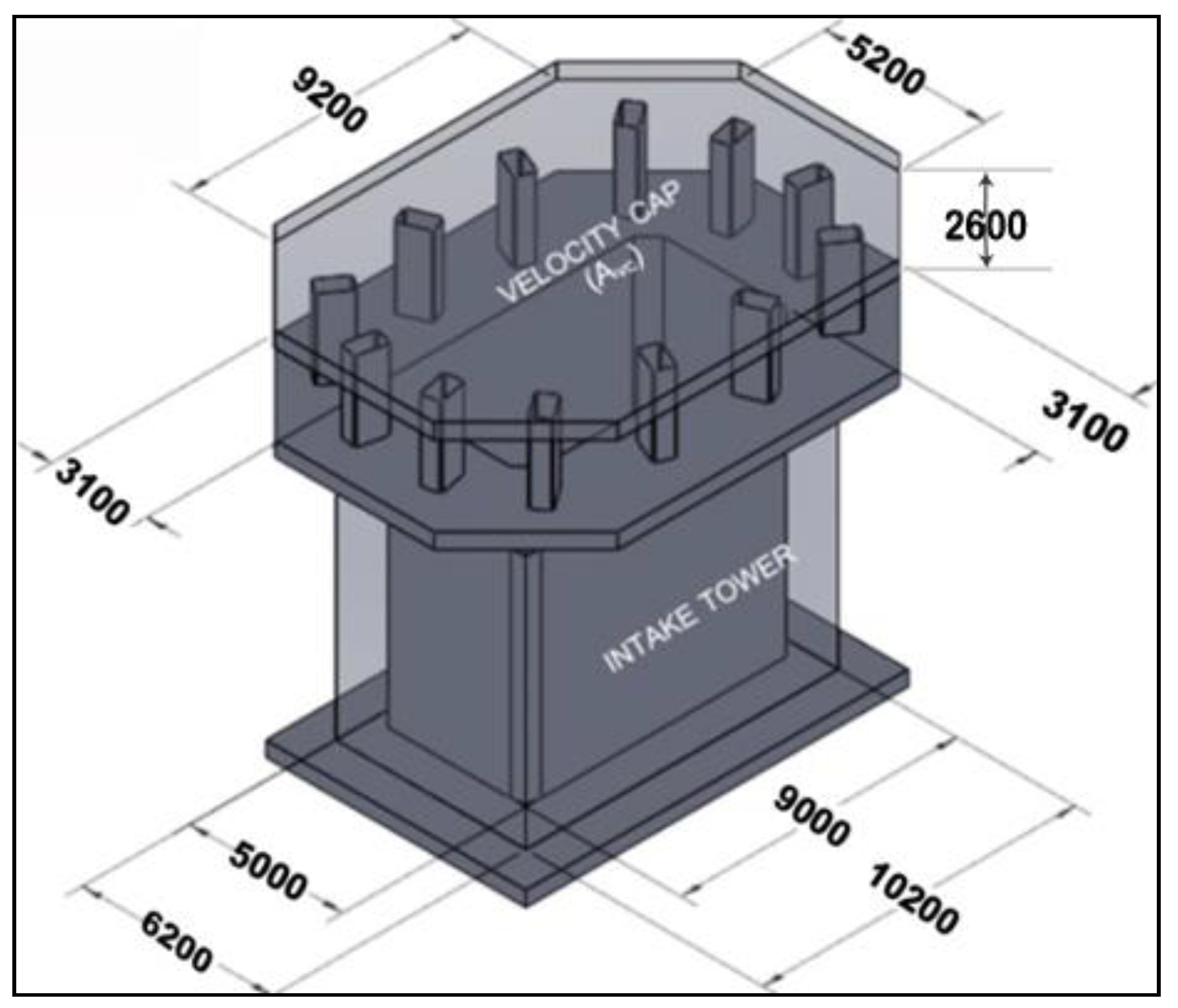
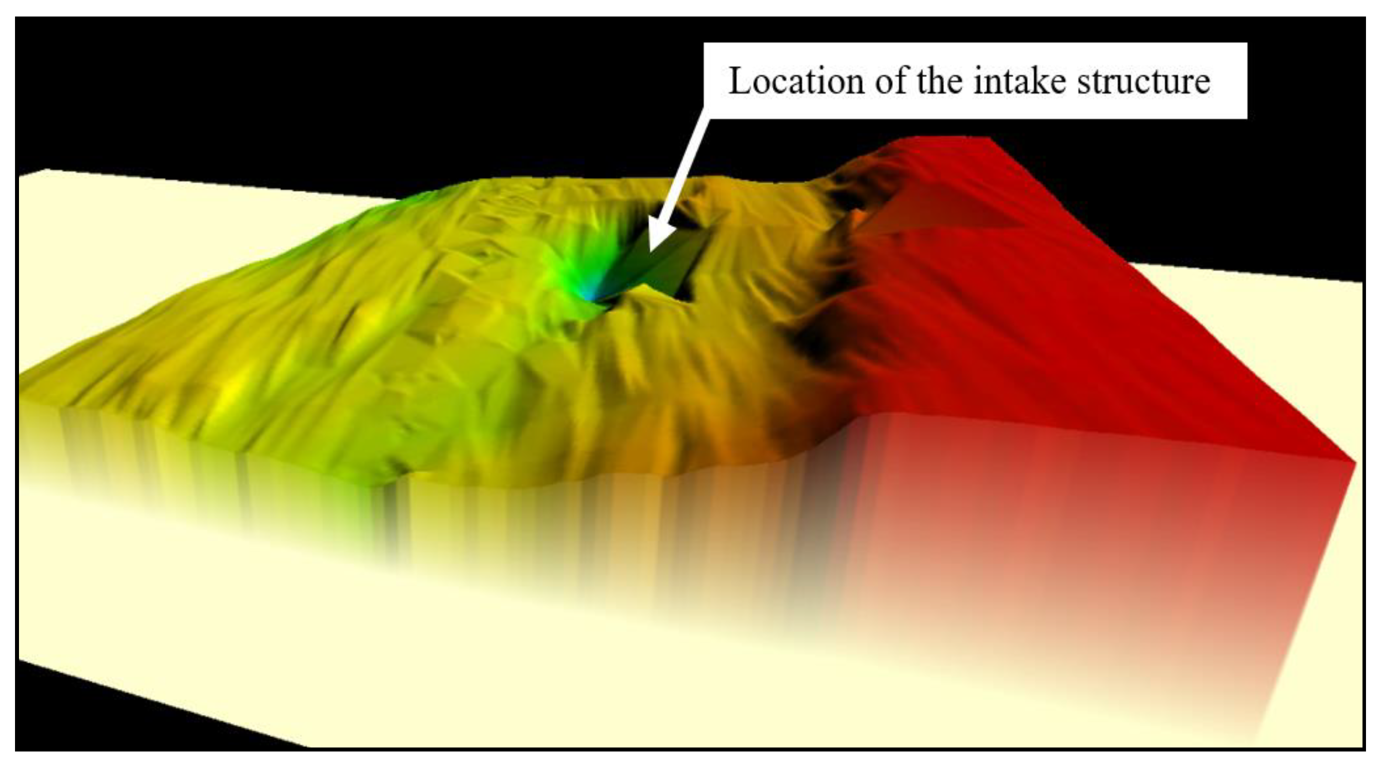
2.2. Model Setup

An existing seawater intake structure was used as a basis for the intake model. The intake structure is fully submerged underwater with a submergence of 2.2 m from mean sea level (MSL) and is extracting water at a rate of 25.43 m³/s. The existing structure is partially buried in the seabed (~4.8 m below the existing seabed level) and the water depth during MSL is approximately 10 m.

The intake structure is composed of 2 major components: velocity cap and intake tower. The velocity cap size of 9.2 m × 5.2 m has 3.1 m horizontal shelf (ℓ_vc) and 2.6 m vertical opening (H_vc) to convey the flow into the intake tower. The intake tower is rectangular in shape with an outer large and long of 6.2 m × 10.2 m. The intake tower opening size is 5 m large × 9 m long. The total height of intake tower is 9.98 m. Figure 3 shows the overall dimensions of the intake structure.

A model with domain sizes of 41 m × 45m × 18 m is constructed for this study. The measured bathymetric data is imported into the model using a universal terrain representation raster format to provide a realistic bed level for modelling. The 3D raster bathymetric map is shown in Figure 4. The intake structure was incorporated into the model bathymetry to mimic the actual site condition.

The boundary condition (BC) of the model domain is defined as velocity, pressure, wall, and mass momentum source. The kinetic energy and dissipation rate are calculated based upon the computational formulas of turbulence quantities at the velocity boundary. The published tidal level [22] is prescribed with pressure-type boundary. The wall boundary is defined at seafloor with no tangential velocities. The model domain is setup with single incompressible fluid with free surface. Fluid fraction (F) = 0 correspond to void region, in which a uniform atmospheric pressure is applied. Mass momentum sinks were added to the intake structure outlet to withdraw water from the model domain. The model boundary conditions are illustrated in Figure 5. One downside regarding the methodology is that the wave effects are not considered in this study. Further data collection would be needed to determine exactly how the wave effects affects the engineering design criteria for the intake structure.

2.3. Mesh Sensitivity Study

Mesh sensitivity study was performed for three computational grids that consisting of 355,296 (M1), 792,028 (M2), and 1,682,826 (M3) nodes. It is suggested by ASME (2009) [23] that the grid refinement should be conducted systematically, and it is highly recommended that the grid refinement factor, r = h_coarse/h_fine, (where h is the grid size) should be greater than 1.3 for most practical problems.

Table 1. Tested gird for mesh sensitivity study.

	Tested Grid	Coarse Grid (M1)	Medium Grid (M2)	Fine Grid (M3)
Grid Info
Total grid cells		355,296	792,028	1,682,826
Min. grid size (h)		0.29	0.22	0.17
Max. grid size (h)		0.52	0.40	0.31
Grid refinement factor (r)			hM1/hM2 = 1.3	hM2/hM3 = 1.3

summarizes the grid information for the tested grid. An extraction rate of 25.43 m³/s is added as mass momentum source, and the intake velocity is recorded at four intake windows. Mesh independent solutions are achieved when the differential between two intake velocities (M1-M2 and M2-M3) is less than +/−0.01 m/s.

Table 2. Comparison of intake velocity for M1, M2, and M3 grids.

Tested Grid	No. Grid Cells	Intake Velocity (m/s)
		Short Window 1	Differential (M2−M1) (M3−M2)	Short Window 2	Differential (M2-M1) (M3-M2)
Coarse Grid (M1)	355,296	0.21		0.23
Medium Grid (M2)	792,028	0.24	0.03	0.24	0.01
Fine Grid (M3)	1,682,826	0.23	−0.01	0.24	0.00
Tested Grid	No. grid cells	Long Window 1	Differential (M2-M1) (M3-M2)	Long Window 2	Differential (M2-M1) (M3-M2)
Coarse Grid (M1)	355,296	0.26		0.24
Medium Grid (M2)	792,028	0.25	−0.01	0.25	0.01
Fine Grid (M3)	1,682,826	0.26	0.01	0.25	0.00

tabulated the comparison of intake velocity for M1, M2, and M3 grids. The results show that the maximum velocity differences between M1 and M2 grid is 0.03 m/s. By increasing the grid resolution, the results show a reduction in velocity differences. The maximum velocity differences between M2 and M3 is generally less than 0.01 m/s. This indicates that the M2 grid has reached a solution value that is independent of the grid resolution. Therefore, the optimum grid is M2 with resolution ranging between 0.22 m and 0.4 m.

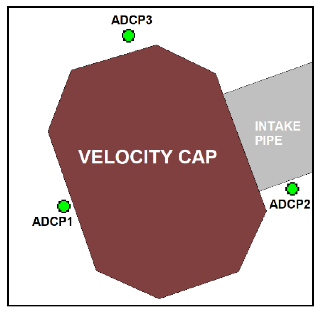
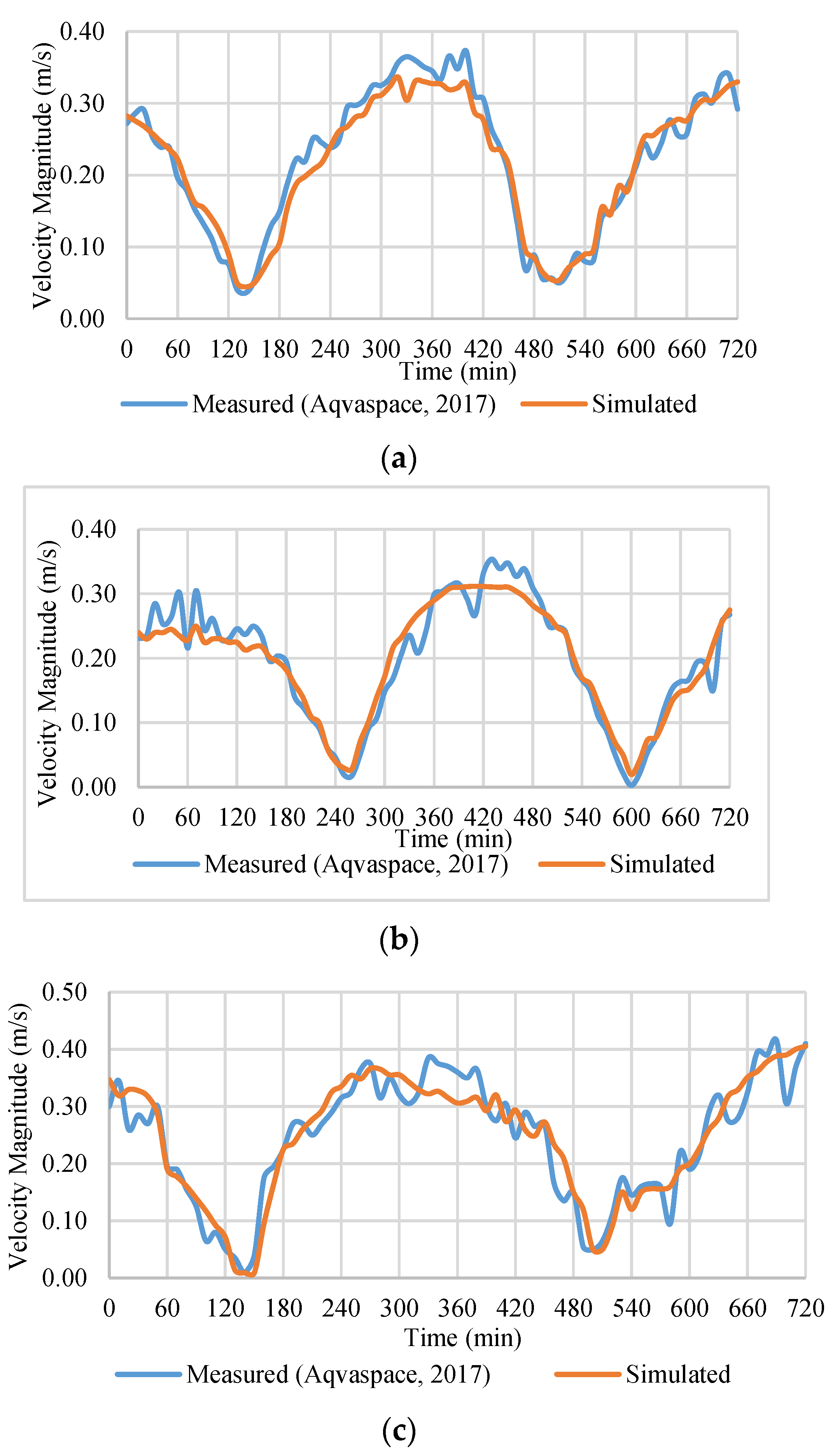
2.4. Model Validation

Secondary velocity measurements were adopted for model validation. The tide at the Penang Strait is semi-diurnal with two high tides and low tides in a tidal day with comparatively little diurnal inequality. The measurements, covering both high and low tides, were captured by three Acoustic Doppler Current Profilers (ADCP1, ADCP2 and ADCP3). ADCP1, ADCP2, and ADCP3 were respectively located at 0.5 m, 2 m, and 1 m from the velocity cap as illustrated in Figure 6. The high resolution FLOW3D CFD model was used to reproduce velocity at these locations. The simulated velocity was validated with the measured data, and the results are graphically shown in Figure 7. It is plausible that slightly higher error percentages will be obtained when the validation results are based on field surveys where data was collected in an uncontrolled environment. Department of Irrigation and Drainage (DID) Malaysia suggested the root mean square percentage error (% RMSE) between the measured and simulated data shall be less than 20% for any coastal hydraulic study and impact assessment [24].

Table 3. Comparison of velocity magnitude between simulated and measured data.

Station	%RMSE	r2	MAE (m)
ADCP1	6.81	0.98	0.02
ADCP2	7.16	0.97	0.02
ADCP3	9.63	0.94	0.03

summarizes the discrepancies between the simulated and measured data with % RMSE, squared of Pearson product-moment correlation coefficient (r²) and mean absolute error (MAE). The RMSE percentage of all ADCP locations are less than 10%, and r² are well above 0.9. This demonstrates that the model is capable and suitable to be used for the investigation of flow field around the intake structure.

3. Results and Discussion

The validated model was used to study the intake velocity at the velocity cap. Figure 8 illustrates the flow field around the existing intake structure during flood, ebb, and slack current conditions. During the flood and ebb currents, it can be clearly perceived that the flow field around the intake structure is mainly influenced by the tidal current. The intake structure increases the flow velocity upstream but decreases the flow velocity downstream. The slow flow region is observed leeward of the structure, which could benefit sheltering effects for fishes [25,26]. The tidal flow passing through the intake window is affected by the compressive interference of the intake suction, which generate velocity gradients around the intake windows. However, the velocity gradients around the intake windows are mild during tidal flow and potentially stimulate an avoidance response in fishes, which aids to reduce marine life impingement.

The weakest tidal currents, which happen during slack tides, occur during the transition from flood to ebb currents, and vice versa. At this point of time, the tidal currents decrease rapidly to nearly stagnant and the flow field around the intake structure is mainly attributed by the intake suction. The velocity gradients around the intake windows are strong and could potentially cause the marine life impingement and entrainment. Therefore, slack current condition (with tidal current = 0) will be adopted in this study to derive the fundamental relationship between intake velocity and design parameters of velocity cap.

The design of the velocity cap is influenced by the parameters as illustrated in Figure 9. Basic terminology must first be established to clearly evaluate the intake velocity in this study. For this study, the term “intake velocity” is represented by V₀—the velocity magnitude measured at the vertical opening of the velocity cap. The velocity magnitude was computed with Equation (5) where $u, v$, and $w$. are fluid velocities in the Cartesian coordinate directions (x, y, z) computed from governing equation of FLOW3D.

$$V_0= \sqrt{u^2+v^2+w^2}$$

(5)

To analyze V₀ in the following sections, V₀ profiles were extracted along the vertical openings (H_vc) at the middle of the four windows (two long windows at L/2 and two short windows at W/2, as shown in Figure 2). The intake velocity profile at each window was analysed to determine the average V₀. The term “intake velocity ratio (V_r)” is used in this study to represent the dimensionless velocity that considers the ratio of intake velocity (V₀) to average suction velocity at the intake pipe (V_pipe) (V_r = V₀/V_pipe). V_pipe is determined by using Equation (6), where Q is the intake rate and A_pipe is the pipe area that is calculated with Equation (7). V_r can be used to evaluate the intake structural performance. Lower V_r indicates better structural performance in reducing intake velocy, and vice versa. The use of the dimensionless intake velocity ratio (V_r) is more appropriate and makes the application more generalizable to various intake rates.

$$V_{pipe}=\raisebox{1ex}{$Q$}\!\left/ \!\raisebox{-1ex}{$A_{pipe}$}\right.$$

(6)

$$A_{pipe}= \frac{\pi D_{pipe}{}^2}{4}$$

(7)

3.1. Fundamental Relationships

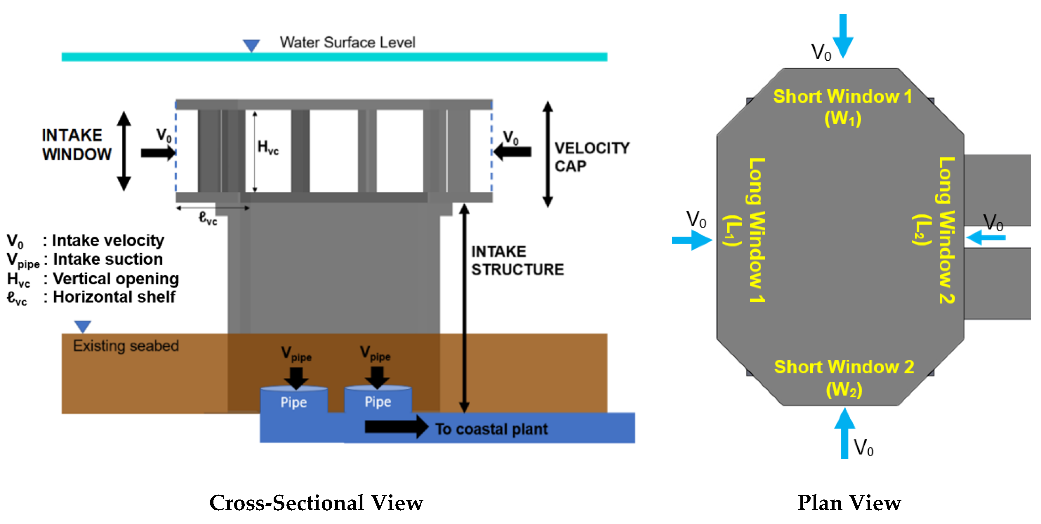
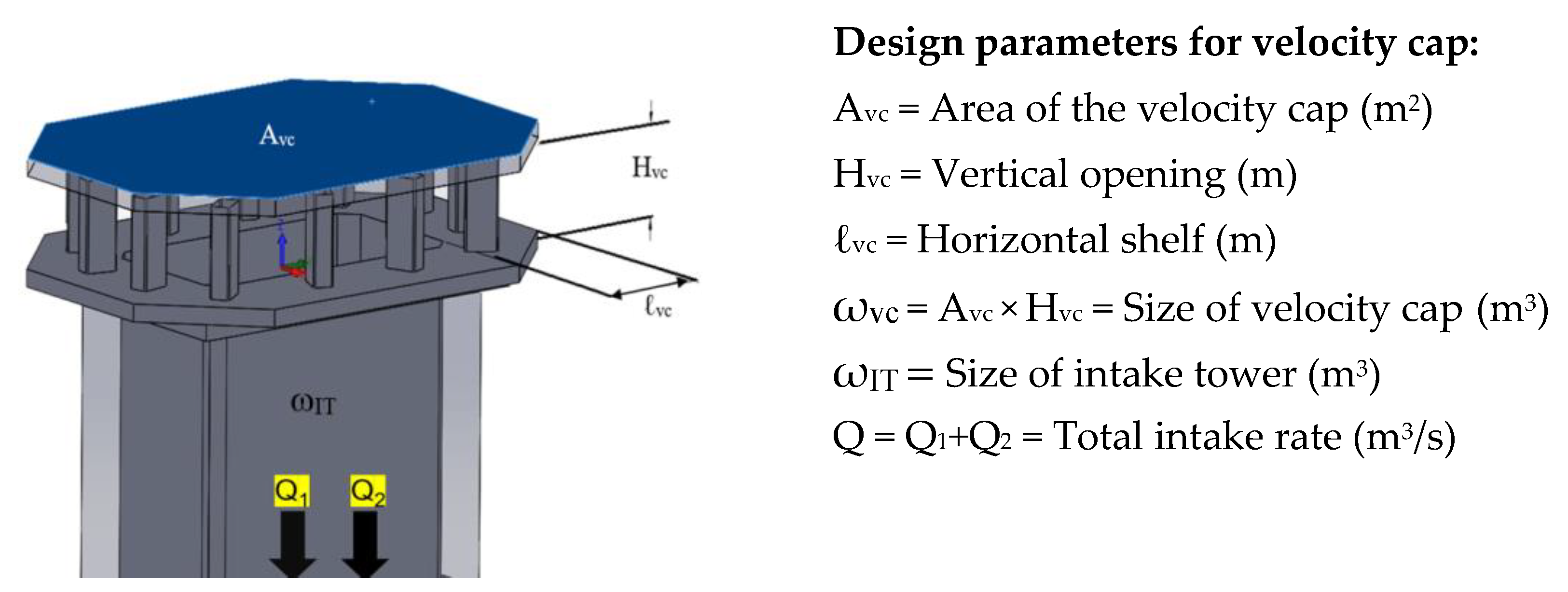
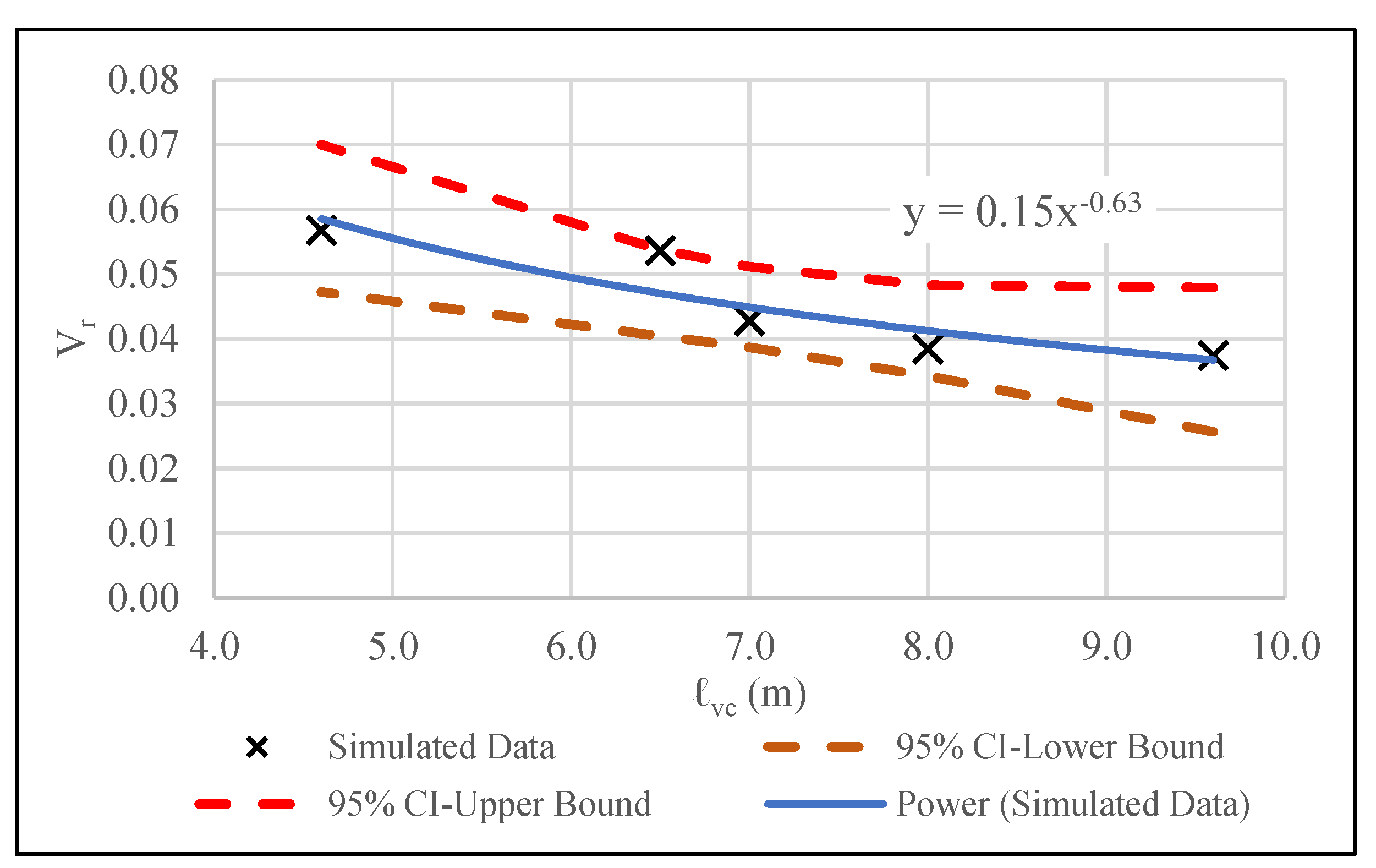
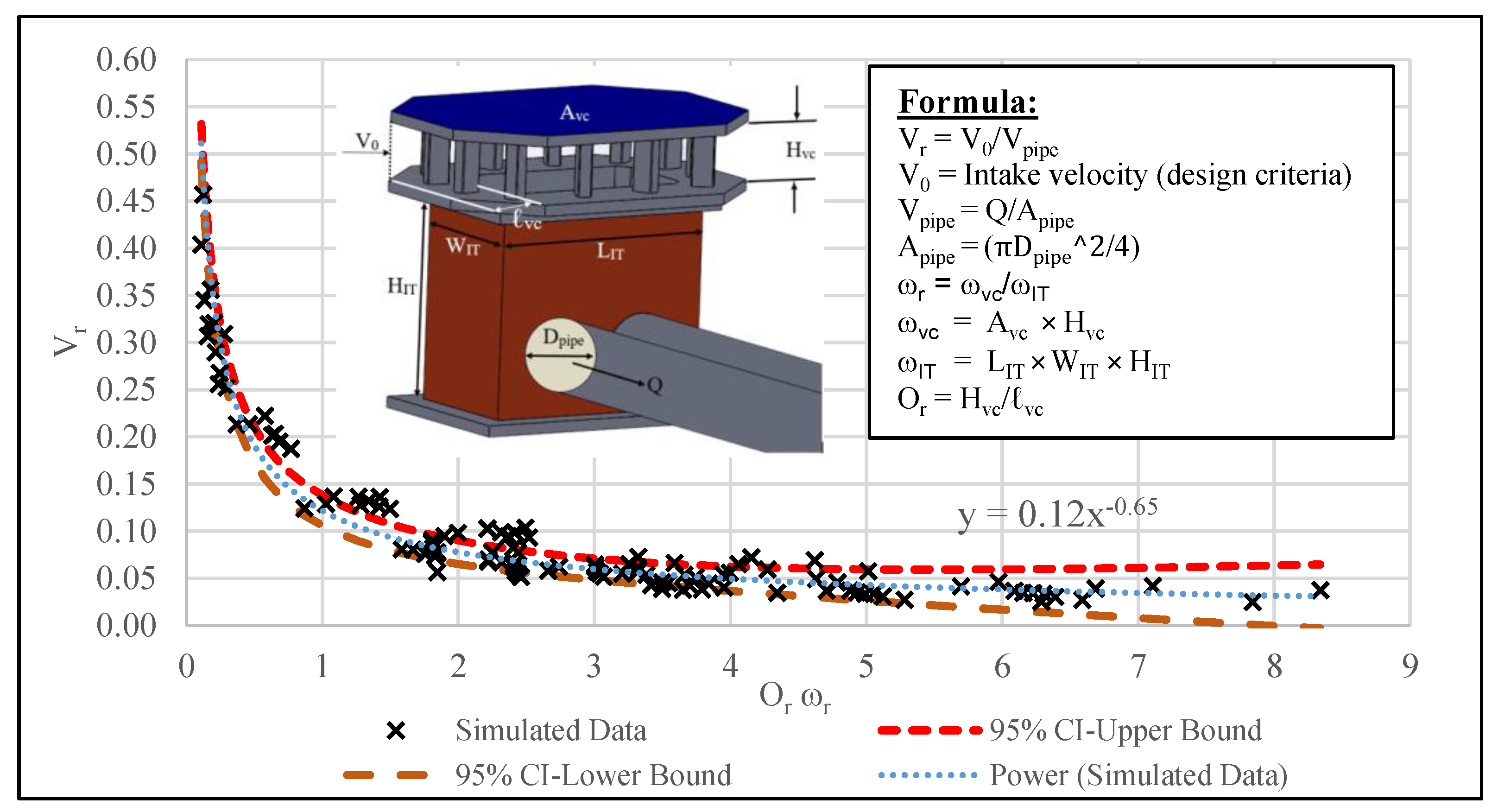
3.1.1. Effect of Horizontal Shelf (ℓ_vc)

A total of five test cases were conducted to evaluate the effect of ℓ_vc on V_r. H_vc and ω_IT in all test cases are respectively set at 5.5 m and 450 m³. A range of intake rates (Q = 45, 50, and 60 m³/s) are considered in this section. The analyzed simulation results are presented in Figure 10 as a scatter plot. The best fit equation and 95% confidence interval (CI) are presented. The results of a regression analysis revealed that V_r and ℓ_vc have a negative non-linear relationship. V_r can be reduced by increasing the length of ℓ_vc. The relationship between V_r and ℓ_vc can be expressed with the power function: V_r = 0.15 ℓ_vc^−0.63. All simulated data are lies within the 95% CI. There is a 95% probability that the best fit equation between V_r against ℓ_vc lies within the confidence interval.

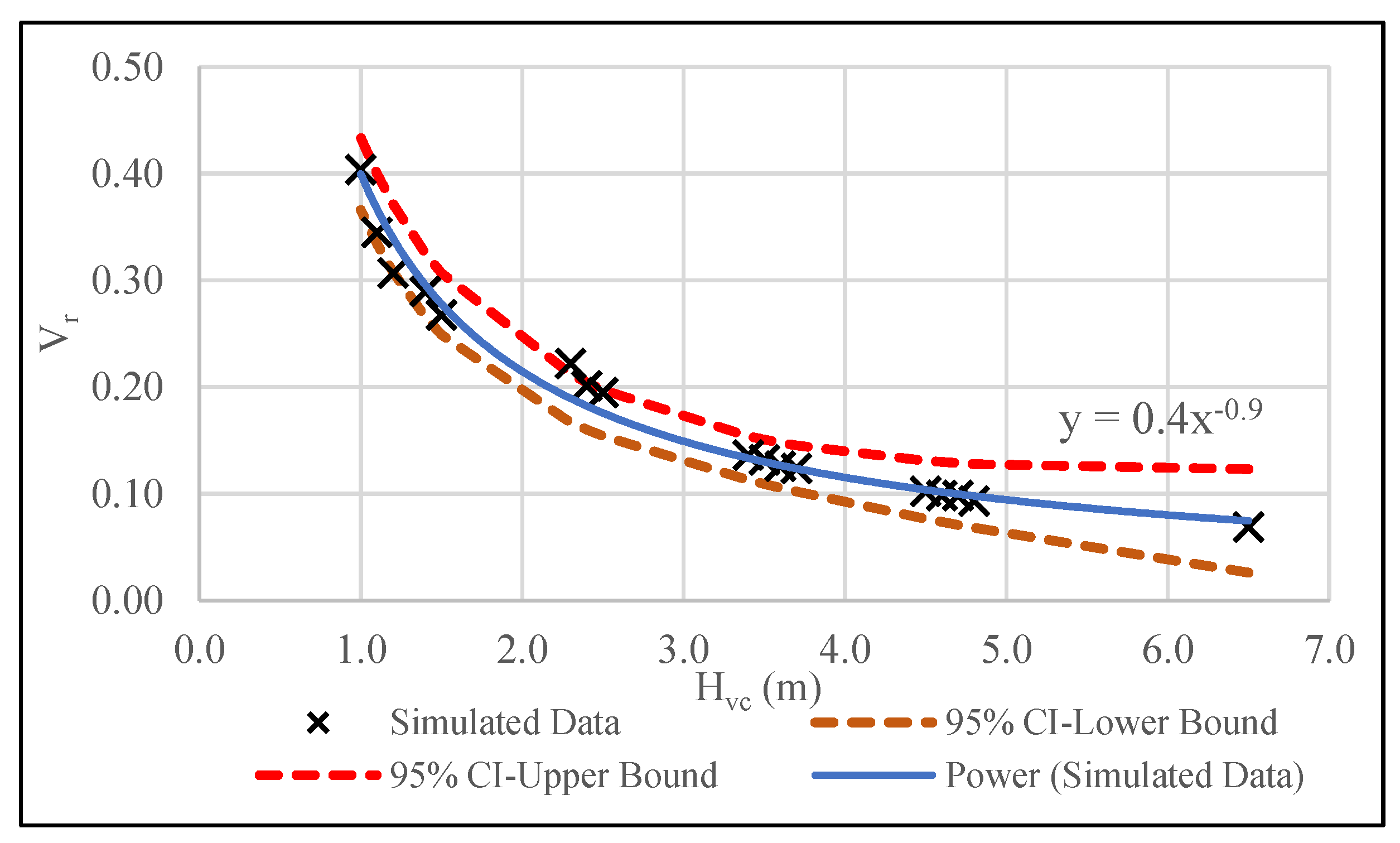
3.1.2. Effect of Vertical Opening (H_vc)

The investigation continued by evaluating the influence of H_vc to V_r, with 17 test cases. ℓ_vc, A_vc, and ω_ΙΤ in all test cases are respectively set at 3.1 m, 152 m², and 450 m³. Intake rate ranging between 6 and 30 m³/s are considered in this section. The analyzed simulation results are presented in Figure 11. The results of regression analysis revealed that V_r and H_vc have a negative non-linear relationship. V_r can be reduced by the increasing H_vc. The relationship between V_r and H_vc can be expressed by the equation: V_r = 0.4H_vc^−0.9. All simulated data are lies within the 95% confidence interval bands. The best fit equations have 95% confidence interval.

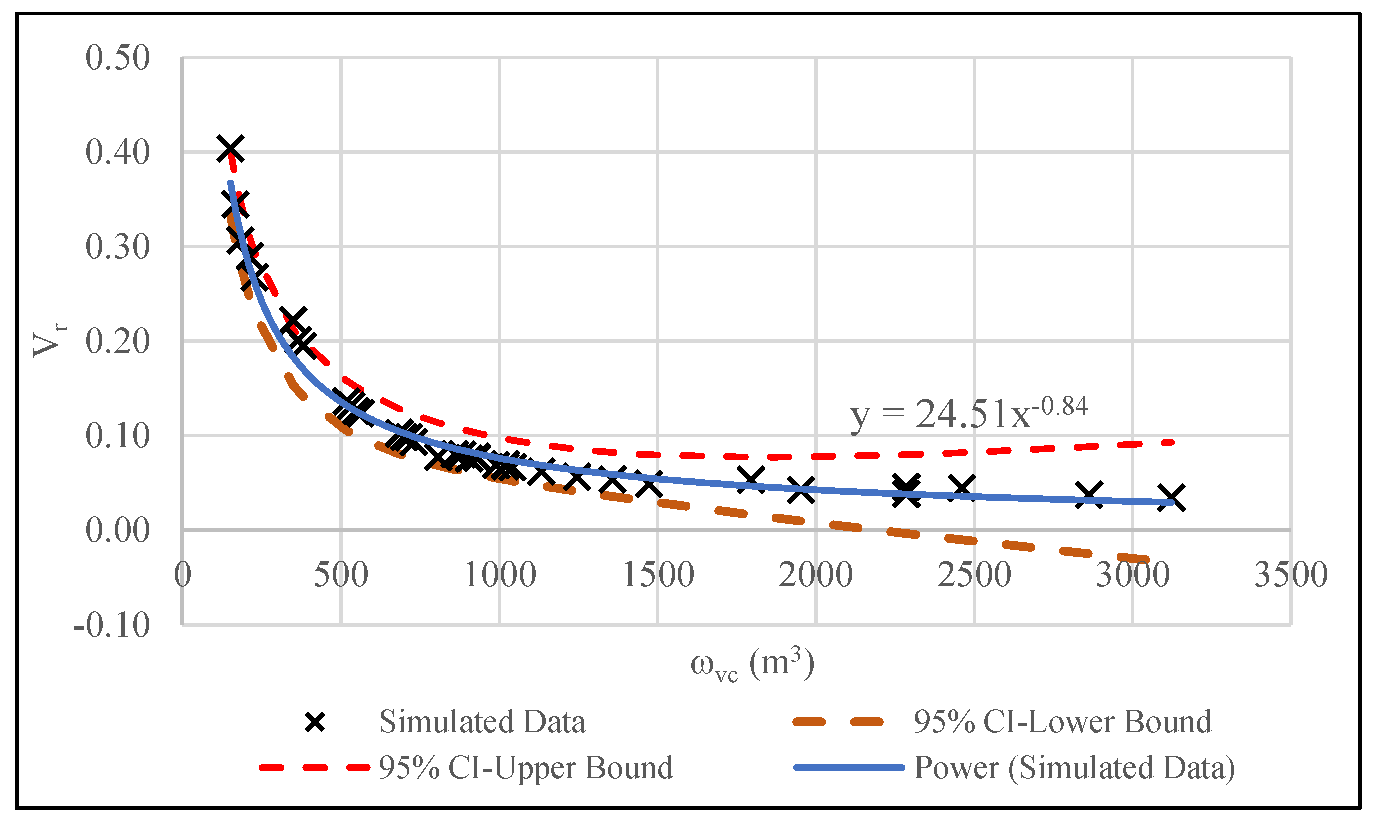
3.1.3. Effect of Velocity Cap Size (ω_vc)

The cumulative influence of the velocity cap design parameters (A_vc, H_vc, and ℓ_vc) to V_r is investigated by using the term “velocity cap size”. The velocity cap size (ω_vc) is calculated by A_{vc ×} H_vc, where A_vc depends upon the velocity cap geometry and is influenced by ℓ_vc. A total of 40 test cases with the following structural design range were adopted in the simulations:

• Intake rate (Q): 6–60 m³/s
• Vertical opening (H_vc): 1.0–6.5 m
• Horizontal shelf (ℓ_vc): 3.1–9.6 m
• Area of the velocity cap (A_vc): 152–520 m²
• Size of velocity cap (ω_vc): 152–3122 m³
• Size of intake tower (ω_ΙΤ): 450 m³

The simulated results are plotted as scatter plot with best fit equation and 95% Confidence interval (CI) bands, as shown in Figure 12. The results of a regression analysis revealed that V_r and ω_vc are fitted by the nonlinear power function with a negative relationship. With the increasing ω_vc, V_r is reduced, and the intake performance is increased. However, it is crucial to note that the influence of ω_vc to V_r is reduced significantly when ω_vc > 1000 m³.

3.2. Engineering Design Criteria

The previous findings indicated the potential application of ℓ_vc, H_vc, and ω_vc to control the intake velocity. In this section, the combined effects of ℓ_vc, H_vc, ω_vc, and ω_IT on V_r are investigated. The volume size (ω) is used in this study to make the application more generalizable to the intake tower that is mostly circular in shape. Based on the normal engineering practice [1], the height of intake tower is mostly ranging between 5 and 9 m for constructability considerations (i.e., seabed bathymetry and distance of the structure from the shore). The term “volume ratio (ω_r)”, where ω_r = ω_vc/ω_IT, used in this section is a dimensionless term to represent the ratio of velocity cap size to intake tower size. The term “Window opening ratio (O_r)”, where O_r = H_vc/ℓ_vc, is a dimensionless term to represent the ratio of vertical opening to horizontal shelf. A total of 115 test cases with the following structural design range were adopted in the simulations:

• Intake rate (Q): 6–60 m³/s
• Vertical opening (H_vc): 1.0–6.5 m
• Horizontal shelf (ℓ_vc): 3.1–9.6 m
• Area of the velocity cap (A_vc): 152–520 m²
• Size of velocity cap (ω_vc): 152–3122 m³
• Size of intake tower (ω_ΙΤ): 240–450 m³

Figure 13 demonstrates the influence of ω_r to V_r. The results of a regression analysis highlighted a strong negative non-linear relationship between the V_r and ω_r. The best fit equation between V_r and ω_r is 0.16ω_r^−0.81 with 95% confidence interval. Majority of the simulated data lies within the upper and lower bounds. It is noted that V_r is reduced by the increasing volume ratio ω_r. However, it is important to note that the influence of ω_r to V_r is insignificant when ω_r > 4. Figure 14 demonstrates the combined effects of O_r and ω_r to V_r. The results of a regression analysis indicated a strong negative non-linear relationship between V_r, O_r and ω_r, with the best fit equation of V_r = 0.12(O_rω_r)^−0.65. A set of design parameter formulations were derived and is summarized in

Table 4. Engineering design criteria for seawater intake structure.

Design Parameter	Symbol	Design Formulation
Intake velocity ratio	Vr	V0/Vpipe where V0 is the design criteria for intake velocity
Pipe velocity (m/s)	Vpipe	Q/Apipe where Q = intake rate (m3/s) and Apipe = πDpipe2/4
Intake opening ratio	Or	$0.36 \times { \mathrm{V}}_{\mathrm{r}}{}^{-0.31}$. where Or = Hvc/ℓvc
Volume ratio	ωr	$0.11 \times V_r^{-1.23}$ where ωr = ωvc/ωIT

Note: The formulations are in SI unit.

.

The main design consideration for a seawater intake structure is the impact on fish impingement at intakes, resulting from intake velocities (V₀). The Environmental Protection Agency (EPA) of the United States (US) has promulgated final ruling under the Clean Water Act to restrict the through-screen velocity (comparable to the term “intake velocity” used in this study) of a water intake structure to a maximum 0.15 m/s, and specify that the intake structures should be equipped with a velocity cap. The intake velocity performance standard proposed by USEPA is specifically referred to as the “design intake velocity”—which can be used to evaluate intake design prior to construction. The regulation of intake velocity by USEPA can thus be a good design reference to indicate a low potential for detrimental impacts from impingement.

4. Conclusions

This study has shown that intake design can greatly influence the intake velocity, and by optimizing the design parameters, it is greatly reducing the intake velocity. Particular attention is paid to seawater intake structures, which typically consists of velocity cap and intake tower. The research findings are generally summarized into the following areas:

(a)

This study has demonstrated the usefulness of velocity cap in mitigating intake velocity. The key design parameters for velocity cap is velocity cap size (ω_vc), which comprises of the horizontal shelf (ℓ_vc) and vertical opening (H_vc). The recommended intake opening ratio (O_r) shall be 0.36V_r^−0.31, where O_r =H_vc/ℓ_vc and V_r =V₀/V_pipe. V_o is the velocity at the intake window and V_pipe is the suction velocity at the intake pipe.

(b)

With increased velocity cap size, the intake velocity is reduced. The volume ratio (ω_r) between the velocity cap (ω_vc) and intake tower (ω_IT) is recommended at 0.11V_r^−1.23.

(c)

The primary environmental impact caused by intake operation is marine life impingement resulting from the intake velocity. Therefore, it is reasonable to regulate intake velocity as an environmental safety factor. However, to the author’s best knowledge, most of the country has no single regulation used to enforce the intake performance for environment protection purposes. Thus, the maximum allowable intake value of 0.15 m/s, used by the United States as their national screening value for the permissible regulation of intake velocity, shall be used as reference to establish engineering design criteria for seawater intake structures. This value has been widely utilized to indicate that an intake structure has low potential adverse environmental impact.

References

- Pita, E. Seawater intakes for desalination plants: Design and construction. In Proceedings of the International Conference on Desalination, Environment and Marine Outfall Systems, Muscat, Oman, 13–16 April 2014. [Google Scholar]
- Voutchkov, N. Design and construction of open intakes. In Sustainable Desalination Handbook: Plant Selection, Design and Implementation; Gude, V.G., Ed.; Elsevier: Oxford, UK, 2018; pp. 201–226. [Google Scholar]
- Lattemann, S.; Höpner, T. Environmental impact and impact assessment of seawater desalination. Desalination 2008, 220, 1–15. [Google Scholar] [CrossRef]
- Pankratz, T. An overview of seawater intake facilities for seawater desalination. In The Future of Desalination in Texas; Biennial Report on Water Desalination, Texas Water Development: Austin, TX, USA, 2004; Volume 2, pp. 1–12. [Google Scholar]
- WateReuse Association. White paper on desalination plant intakes: Impingement and entrainment impacts and solutions. Desalin. Comm. 2011. [Google Scholar] [CrossRef]
- Environmental Protection Agency (EPA). National pollution discharge elimination system—Final regulations to establish requirements for cooling water intake structures at existing facilities and amend requirements at Phase I facilities: Final rule. Fed. Regist. 2014, 79, 48300. [Google Scholar]
- Turnpenny, A.W.H.; Keeffe, N.O. Screening for Intake and Outfalls: A Best Practice Guide; Science Report SC030231; Environment Agency: Bristol, UK, 2005.
- Pankratz, T. Overview of intake systems for seawater reverse osmosis facilities. In Intakes and Outfalls for Seawater Reverse-Osmosis Desalination Facilities: Innovations and Environmental Impacts; Missimer, T.M., Jones, B., Maliva, R.G., Eds.; Springer: New York, NY, USA, 2015; pp. 3–17. [Google Scholar]
- Pita, E.; Sierra, I. Seawater Intake Structures. In Proceedings of the International Symposium on Outfall Systems, Mar del Plata, Argentina, 15–18 May 2011. [Google Scholar]
- Environmental Protection Agency (EPA). Requirements Applicable to Cooling Water Intake Structures for New Facilities under Section 316(b) of the Act; US Electronic Code of Federal Regulations: Washington, DC, USA, 2001; Volume 40.
- Electric Power Research Institute (EPRI). Technical Evaluation of the Utility of Intake Approach Velocity as an Indicator of Potential Adverse Environmental Impact under Clean Water Act Section 316(b); Final Report; EPRI Inc.: Palo Alto, CA, USA, 2000; p. 1000731. [Google Scholar]
- National Marine Fisheries Service (NMFS). Fish Screening Criteria for Anadromous Salmonids; U.S. Department of Commerce, National Oceanic and Atmospheric Administration: Washington, DC, USA, 1997.
- Pearce, R.O.; Lee, R.T. Some design considerations for approach velocities at juvenile salmonid screening facilities. Am. Fish. Soc. Symp. 1991, 10, 237–248. [Google Scholar]
- Schuler, V.J.; Larson, L.E. Improved fish protection at intake systems. J. Environ. Eng. Div. ASCE 1975, 101, EE6. [Google Scholar]
- Moideen, R.; Ranjan Behera, M.; Kamath, A.; Bihs, H. Effect of girder spacing and depth on the solitary wave impact on coastal bridge deck for different airgaps. J. Mar. Sci. Eng. 2019, 7, 140. [Google Scholar] [CrossRef]
- Gomes, A.; Pinho, J.L.S.; Valente, T.; Antunes do Carmo, J.S.; Hegde, A. Performance assessment of a semi-circular breakwater through CFD modelling. J. Mar. Sci. Eng. 2020, 8, 226. [Google Scholar] [CrossRef]
- Karami, H.; Farzin, S.; Sadrabadi, M.T.; Moazeni, H. Simulation of flow pattern at rectangular lateral intake with different dike and submerged vane scenarios. J. Water Sci. Eng. 2017, 10, 246–255. [Google Scholar] [CrossRef]
- Ruether, N.; Singh, J.M.; Olsen, N.R.B.; Atkinson, E. 3D computation of sediment transport at water intakes. In Proceedings of the Institution of Civil Engineers: Water Management; Thomas Telford Ltd.: London, UK, 2005; Volume 158, pp. 1–8. [Google Scholar]
- Aqvaspace Sdn. Bhd. Marine Data Collection around Perai CCGT Power Plant, Penang; Survey report: AQSP/RPT/07-2017/G&P/DTC/10096; Aqvaspace Sdn. Bhd.: Selangor, Malaysia, 2017; pp. 1–54, Unpublished Report. [Google Scholar]
- Chie, L.H.; Abd Wahab, A.K.; Yapandi, F.K.M. Performance of different turbulence models in predicting flow kinematics around and open offshore intake. SN Appl. Sci. 2019, 1, 1266. [Google Scholar]
- Yakhot, V.; Smith, L.M. The renormalization group, the e-expansion and derivation of turbulence models. J. Sci. Comput. 1992, 7, 35–61. [Google Scholar] [CrossRef]
- Royal Malaysian Navy. Tide Table Malaysa: Volume 1; National Hydrographic Centre: Klang, Selangor, Malaysia, 2017.
- American Society of Mechanical Engineers (ASME). Standard for Verification and Validation in Computational Fluid Dynamics and Heat Transfer; ASME: New York, NY, USA, 2009. [Google Scholar]
- Department of Irrigation and Drainage (DID). Guidelines for Preparation of Coastal Engineering Hydraulic Study and Impact Evaluation; Department of Irrigation and Drainage: Kuala Lumpur, Malaysia, 2001.
- Liu, Y.; Zhao, Y.P.; Dong, G.H.; Guan, C.T.; Cui, Y.; Xu, T.J. A study of the flow field characteristics around star-haped artificial reefs. J. Fluids Struct. 2013, 39, 27–40. [Google Scholar] [CrossRef]
- Liu, T.L.; Su, D.T. Numerical analysis of the influence of reef arrangements on artificial reef flow fields. Ocean Eng. 2013, 74, 81–89. [Google Scholar] [CrossRef]