Article

Prediction of Ocean Weather Based on Denoising AutoEncoder and Convolutional LSTM

1
Research Institute of Marine Systems Engineering, Seoul National University, Seoul 08826, Korea
2
Department of Naval Architecture and Ocean Engineering, Seoul National University, Seoul 08826, Korea
3
Research Institute of Marine Systems Engineering, Seoul National University, Seoul 08826, Korea
4
Digitalization Team, Korean Register, Busan 46762, Korea
5
ICT Solution Team, Korean Register, Busan 46762, Korea
*
Author to whom correspondence should be addressed.
J. Mar. Sci. Eng. 2020, 8(10), 805; https://doi.org/10.3390/jmse8100805
Submission received: 7 August 2020 / Revised: 22 September 2020 / Accepted: 14 October 2020 / Published: 16 October 2020
(This article belongs to the Special Issue Smart Technologies for Shipbuilding)

Abstract

:
The path planning of a ship requires much information, and one of the essential factors is predicting the ocean environment. Ocean weather can generally be gathered from forecasting information provided by weather centers. However, these data are difficult to obtain when satellite communication is unstable during voyages, or there are cases where forecast data for a more extended period of time are needed for the operation of the fleet. Therefore, shipping companies and classification societies have attempted to establish a model for predicting the ocean weather on its own. Historically, ocean weather has been primarily predicted using empirical and numerical methods. Recently, a method for predicting ocean weather using deep learning has emerged. In this study, a deep learning model combining a denoising AutoEncoder and convolutional long short-term memory (LSTM) was proposed to predict the ocean weather worldwide. The denoising AutoEncoder is effective for removing noise that hinders the training of deep learning models. While the LSTM could be used as time-series inputs at specific points, the convolutional LSTM can use time-series images as inputs, making them suitable for predicting a wide range of ocean weather. Herein, using the proposed model, eight parameters of ocean weather were predicted. The proposed learning model predicted ocean weather after one week, showing an average error of 6.7%. The results show the applicability of the proposed learning model for predicting ocean weather.

Graphical Abstract

1. Introduction

1.1. Research Background

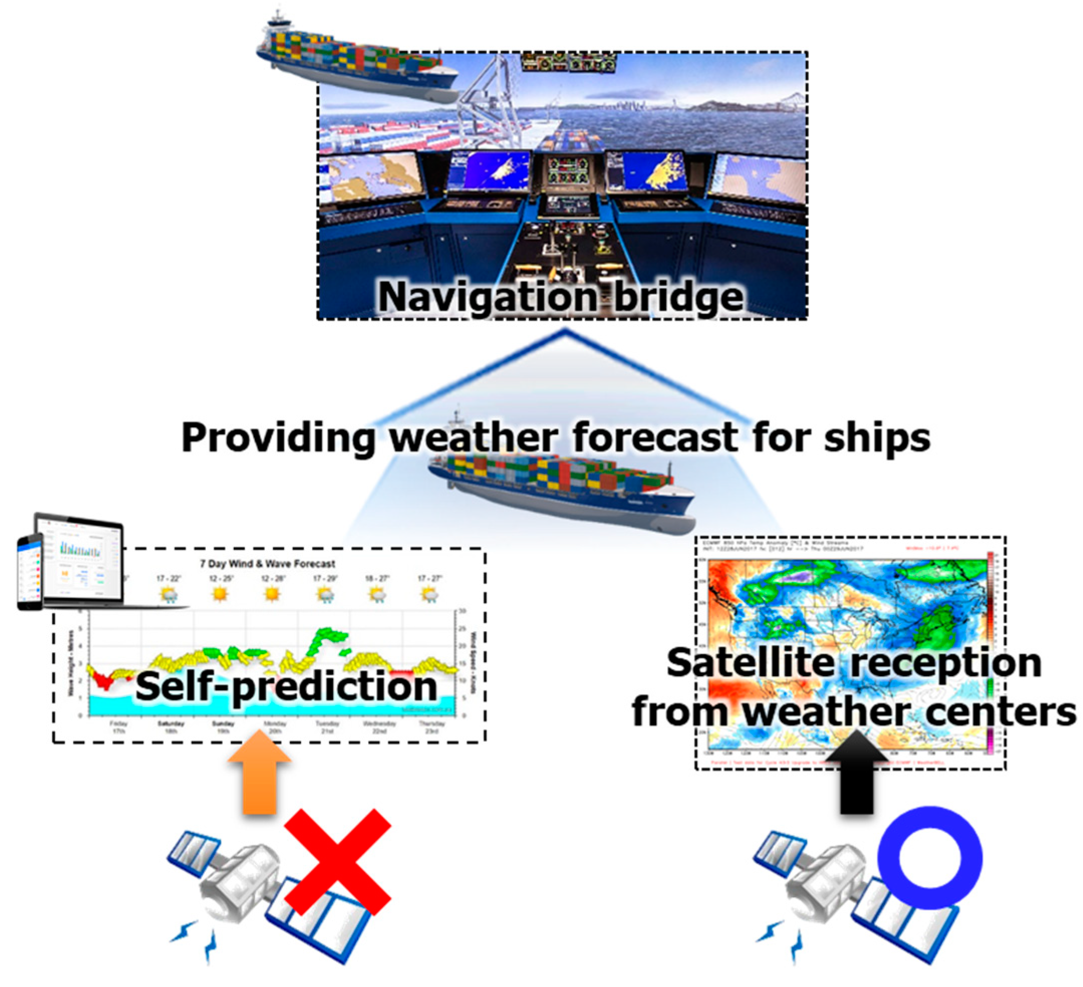
Ocean weather is one of the key considerations for robust ship path planning. The resistance of a ship can be divided into the still water resistance exerted by principal dimensions and the hull form of the ship, and an additional resistance exerted by ocean weather. The still water resistance is estimated during the design of the ship, and the additional resistance changes each time, depending on the ocean weather. Therefore, ocean weather data are used to calculate the additional resistance. For calculating the additional resistance, ISO15016:2015 [1], which is a guideline for the calculation of ship power, can be used. According to this guideline, wave height, wave direction, wave period, wind speed, wind direction, current speed, current velocity, and sea temperature are required to calculate roughly the required power of the ship in the sea. By adding this resistance to the still water resistance, the total resistance of the ship can be calculated. Using the total resistance, the required power and fuel consumption of the ship can be estimated. To accomplish this, shipping companies and classification societies obtain ocean weather from weather centers. Currently, with the introduction of new technologies, path planning is being implemented in various ways for shipping companies. Predicting ocean weather is also essential in this process. Under normal circumstances, forecast data from weather centers can be acquired via satellite communication. However, in situations where data transmission and reception are not stable, the weather should be predicted without outside assistance. In addition, typical weather centers provide approximately 6 weeks of forecast data. Satellite communications are rarely lost for periods longer than 6 weeks. However, if there is no reception of the forecast data for the ocean weather, even for a short period of time, we have no choice but to rely on predicted information which is received before the loss of connection. In addition, typical forecasting information has a characteristic that the longer the forecast period, the greater the error. Therefore, in order to get even slightly more accurate data, it is necessary to have its own prediction model. On the other hand, control centers also need to pay regular fees to receive real-time forecasting information from weather centers. Therefore, we can reduce these costs by building our own prediction model. Figure 1 shows the necessity of self-predicting ocean weather.
In general, “empirical and numerical methods are used for weather forecasting” [2]. Therefore, each weather center has a prediction model that uses its own analysis and weather data stored for a long time. However, because shipping companies and classification societies do not have such data and long-term experience with weather forecasting, there are limitations in developing prediction models in the same way as weather centers. Therefore, “as a requirement for any forecast, an appropriately representative model should be developed, calibrated, and validated” [3]. To accomplish this, various methods have been proposed, including data-driven approaches. One of the methods that has been recently highlighted is deep learning. Deep learning is an effective approach to grasp the causality of data in situations with insufficient experience and to derive meaningful prediction models. Therefore, in this study, deep learning was used to predict ocean weather.

1.2. Related Works

Several studies have predicted ocean weather using machine learning. Jain et al. [4] predicted wave height using three methods: an artificial neural network (ANN), genetic programming (GP), and model tree (MT). For the ANN, a deep feed-forward network (DFN), which is a comparatively simple configuration, was used. The three methods were used to predict wave height in the Arabian Sea from 3 to 72 h. As a result of predicting the significant wave height after three days using three models, the mean absolute error (MAE) was found to be from 0.19 to 0.40 m. The study demonstrated that GP and MT are more competitive methods than ANN, as the time-series characteristics of the weather data are not considered using the basic DFN. Mahjoobi et al. [5] studied about three parameters of weather data: significant wave height, peak spectral period, and mean wave direction. They used three models to predict weather data in Lake Ontario: an ANN, an adaptive-network based fuzzy inference system (ANFIS), and a fuzzy inference system (FIS). As a result of performing predictions for three ocean weather, the mean squared error (MSE) for the significant wave height was 0.14 to 0.18 m, the peak spectral period was 0.74 to 1.16 s, and the mean wave direction was 2543° to 2893°, respectively. They concluded that the ANFIS model was marginally more accurate than the other models. However, they did not consider the time-series characteristics of the weather data. That is, they did not consider the characteristics of ocean weather that change over time. Similarly, Gunaydin [2] studied a method for hindcasting wave height in the Atlantic Ocean using various configurations of an ANN model. He found that the wind speed had the strongest effect on wave height prediction. As a result of predicting the wave height, the MSE was 0.051 to 0.072 m. As mentioned previously, this result has a similar problem regarding the weather data. Zhang et al. [6] predicted sea surface temperature (SST) using a long short-term memory (LSTM) model for coastal seas near China from 1 day to 1 month. They considered the characteristics of the periodicity of the data using the LSTM model. The result was compared with two classical regression methods: support vector regression and multi-layer perceptron regression. As a result of predicting the SST after three days by the proposed method, the root mean square error (RSME) was 0.18°. The study showed that the LSTM was adequate for predicting the periodic data. James et al. [3] predicted the significant wave height, wave period, and wave direction using multi-layer perceptron (MLP) and support vector machine (SVM) [7] models for Monterey Bay in the USA. As a result of predicting three ocean weather events with their model, the RMSE for the significant wave height was 0.41 to 1.62 m, the wave period was 0.45 to 4.08 s, and the wave direction was 12° to 104°, respectively. They compared the results of the two numerical models, and the machine learning showed similar accuracy to a physics-based numerical model.
As mentioned previously, various deep learning methods have been used to predict ocean weather. However, most of them do not consider the periodicity, and only limited information and areas were predicted. To provide ocean weather for shipping companies and classification societies, a general prediction model capable of predicting eight parameters of ocean weather worldwide is required. Therefore, in this study, an image-based prediction model was proposed. Table 1 summarizes and compares related works and this study.

2. Theoretical Background

In this study, we propose a prediction model that can provide ocean weather for ship path planning. The model was developed using deep learning, particularly machine learning. The model predicts eight parameters of ocean weather (i.e., SST, wave height, wave period, wave direction, wind speed (U component), wind speed (V component), current speed (U component), and current speed (V component)) worldwide. For this, an advanced model should be used, rather than a general deep neural network. Therefore, a denoising AutoEncoder and convolutional LSTM (simply, ConvLSTM) that can train 2D time-series data were used. To predict ocean weather for the entire world, the ConvLSTM, which can set the input data as a large area, was used. In addition, if the ConvLSTM is used, each parameter of ocean weather can be used as a channel image; hence, it is possible to predict the ocean weather by considering the causality for each other. Secondly, if the training of models is performed using limited training data, the delayed prediction problems may occur. It can be solved by using AutoEncoder. Therefore, we proposed a prediction model that combines the AutoEncoder and the ConvLSTM. This section introduces the process from essential deep neural networks to the convolutional LSTM and the AutoEncoder.

2.1. Conventional Long Short-Term Memory (LSTM)

The DFN, which is the basic model of deep learning, consists of an input layer, hidden layers, and an output layer. This configuration is useful for finding an output value based on input values. However, it is not suitable for predicting data over the time series. Therefore, a recurrent neural network (RNN) has been proposed to train data with time series [8]. An RNN is a type of deep learning model in which a hidden node is connected to a directed edge to form a cyclic structure called a directed cycle. It is a model suitable for predicting sequentially arranged data, such as voice and text. In the RNN, the state of the previous time step is used in the next step, and the resulting value is affected by the earlier state. Among various RNN models, we used the LSTM to avoid the gradient vanishing. There are many examples of learning time-series data using the DFN, and the structure is also very simple. However, ocean weather has a complex causality between time, space, and parameters of oceanic weather. In addition, since it has periodicity over a long period of time, it can be said that the LSTM is more suitable than the DFN to understand these characteristics. Many deep learning methods have been developed to train time-series data. Among them, LSTM is the most used to date [9]. Figure 2 shows the configuration of the LSTM and details of the cell state “A”.
The cell state serves as a type of conveyor belt. Therefore, even if the state has elapsed for a long time, the gradient of the input value can be propagated relatively well. The formula of LSTM cell state “A” is shown in Equations (1)–(6).
f t = σ ( W x f x t + W h f h t 1 + b f )
i t = σ ( W x i x t + W h i h t 1 + b i )
o t = σ ( W x o x t + W h o h t 1 + b o )
g t = tanh ( W x g x t + W h g h t 1 + b g )
c t = f t c t 1 + i t g t
h t = o t tanh ( c t )
In Equations (1)–(6), σ is the sigmoid function, W is the weight for each layer (subscription is expressed for input and output layers), xt is the input in time step t, b is the bias (subscription is expressed for gates), and tanh is a hyperbolic tangent function. In Equations (5) and (6), ⨀ is the Hadamard product operator [10]. The forget gate ft is a gate to forget past information. The value obtained by taking the sigmoid after receiving ht−1 and xt is the value that the forget gate sends out. The output range of the sigmoid function is from 0 to 1. If the value is 0, information from the previous state is forgotten, and if it is 1, information from the previous state is completely remembered. The input gate itgt is a gate for storing current information. It takes ht−1 and xt and applies the sigmoid function. Then, the value that takes the hyperbolic tangent (tanh) function and Hadamard product operation is sent from the input gate. Since the range of it is from 0 to 1 and the range of gt is from −1 to 1, each represents the intensity and direction of storing current information.
Since the ocean weather has three causalities (i.e., causality with the ocean weather at the previous time, causality between the parameters of ocean weather, and causality between spaces), three types of causalities for a good prediction model should be considered. Using LSTM, time-series causality can be solved. To solve the other two causalities, the ocean weather should be input at all points where training is desired as vector xt. As the size of the area to be trained increases, the input data vector becomes increasingly exponential. In addition, considering the matrix operation required for learning, performing such a task is practically impossible. To address this problem, LSTM requires a spatial element—that is, a method that can be used as 2D data input.

2.2. Convolutional LSTM

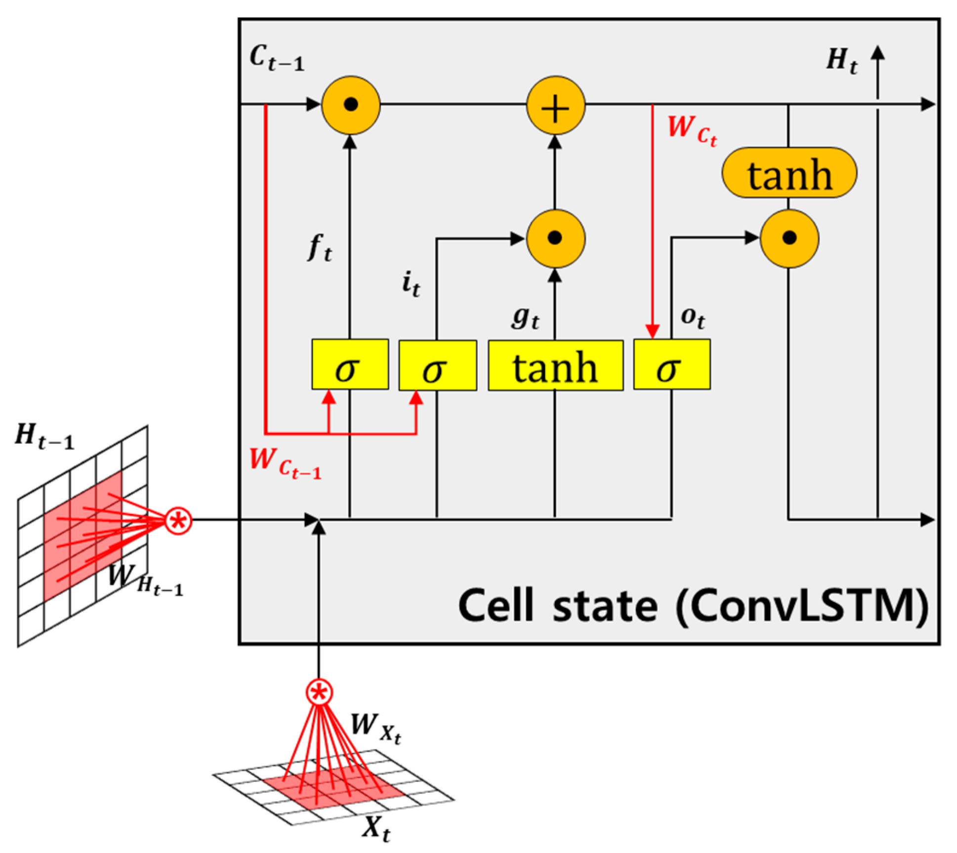
To consider spatial causality in learning, 2D data (image) should be used as input. As described previously, 2D data have a feature that even when the size is increased only slightly, the dimension of the data is significantly increased during training, such as calculating the weight of models. Therefore, a convolutional neural network (CNN) [11], one of the deep learning methods that is used to consider the characteristics of images, can be employed in the LSTM learning model. The most common technique involves a long-term recurrent convolutional (LRCN) network [10], where each 2D feature vector is first extracted by the CNN and used as an input of the LSTM. The difference between the LSTM and the LRCN networks is that the latter (LRCN) passes the input through a convolutional layer. Then, the input data can be an image, that is, 2D data. However, when using 2D data from multiple channels as input data, a 3D tensor is used as input, and feature vectors extracted through the CNN also need to undergo the same process inside as the LSTM. Therefore, it is not suitable for training long-range data, such as ocean weather. However, the ConvLSTM [12] uses an entirely different approach. By performing the LSTM internal operation itself as a convolutional operation, the amount of computation can be dramatically reduced. Figure 3 shows the internal cell state of the ConvLSTM.
The modified key equations in the ConvLSTM can be expressed as Equations (7)–(12).
f t = σ ( W X f * X t + W H f * H t 1 + W c f C t 1 + b f )
i t = σ ( W X i * X t + W H i * H t 1 + W C i C t 1 + b H i )
g t = tanh ( W X g * X t + W H g * H t 1 + b h _ g )
C t = f t C t 1 + i t g t
o t = σ ( W X o * X t + W H o * H t 1 + W C o C t + b h _ o )
H t = o t tanh ( C t )
Equations (1)–(6) and Equations (7)–(12) are quite similar when compared. However, there are two crucial differences. First, in the ConvLSTM, the input gate i, forget gate f, output gate o, cell input X, cell output C, and cell state H are all 3D tensors. This is different from the original LSTM, where all elements were 1D vectors. Second, in the term where matrix multiplication was performed, all matrix multiplications are replaced by convolution operations. This indicates that the number of weights present in all W in each cell may be markedly less than in LSTM. This is the same as the effect when the fully connected layer is replaced by a convolutional layer; it can reduce the number of weights of the model significantly and is suitable for effectively training a large amount of data. Therefore, in this study, the ConvLSTM was used for the ocean weather, which is a very long-range and large scale.

2.3. Denoising AutoEncoder

In general, when training time-series data, a delay prediction problem [13] occurs. When the data are insufficient, or the pattern of the data cannot be identified, it tends to bring values similar to the current value. When the prediction model is overfitted on the input data, if we put an input at a specific point in time, there is a problem of just shifting the data at that point in time. This is referred to as a delayed prediction problem.
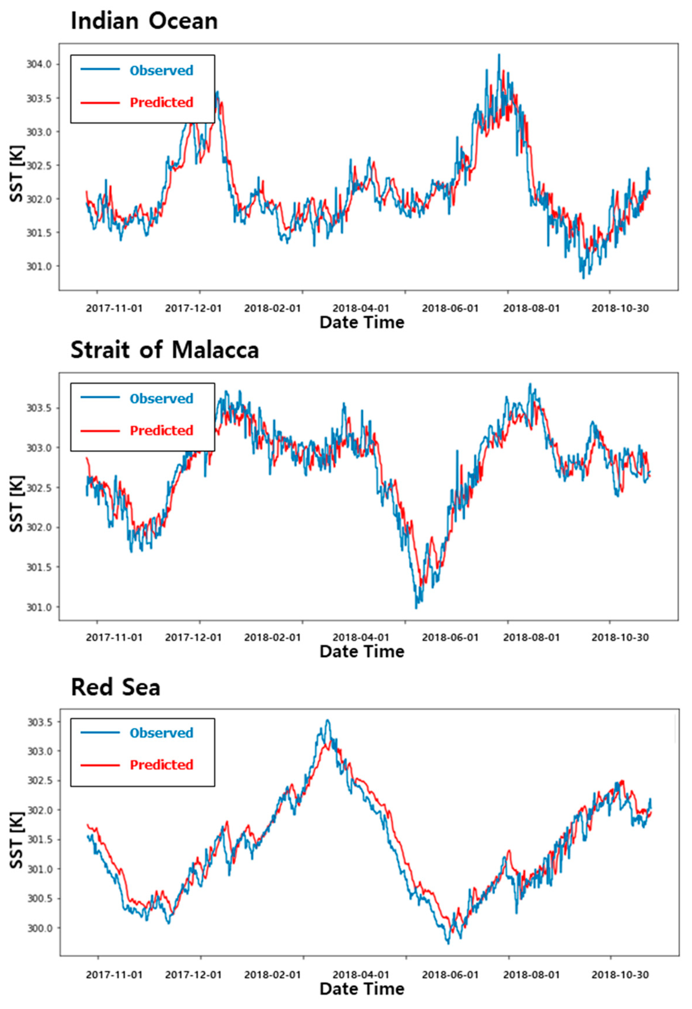
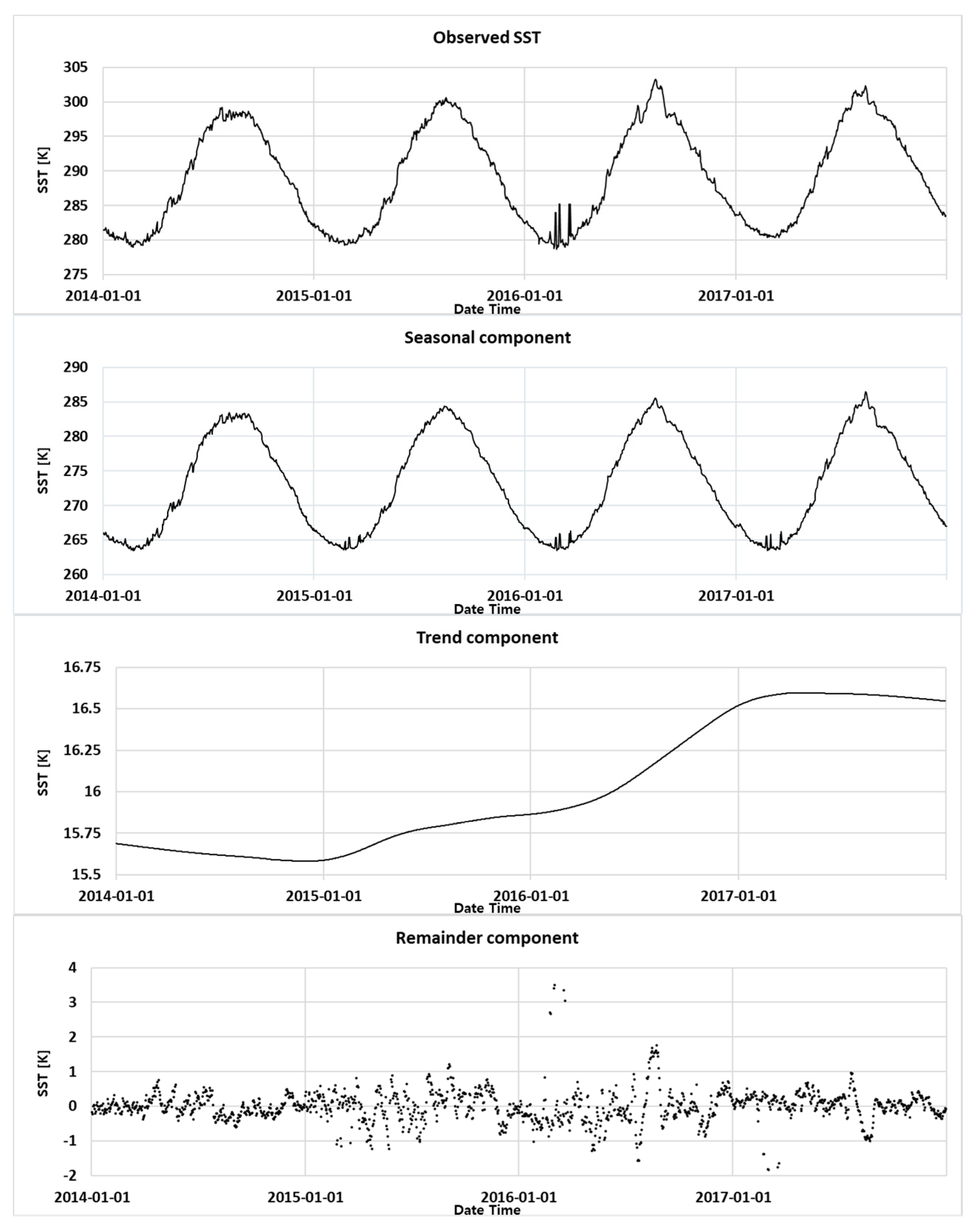
Figure 4 shows the delayed prediction results of SST. We trained a model to predict SST after 5 days using 60 days of data and applied it to three different ocean areas. For training of the prediction model, data collected from the European Center for Medium-Range Weather Forecasts (ECMWF) was used, and a total of eight years of data was used for training. Among them, the initial six years were used for learning, and two years were used as a test set. We performed the training using conventional LSTM based on the data for a point in the region included in Figure 4. As shown in Figure 4, it can be seen that the delayed prediction problem occurred clearly in all graphs. The same problem can also be found in other studies [4,14]. The graphs show that the actual result and the predicted patterns are very similar, although there is a slight difference. Further, it seems that the predicted result has a phase shift with respect to the origin. The delay prediction problem is mostly caused by not being able to understand the data patterns properly. Using all of the predictors required for prediction as input can also be a way to solve the delayed prediction problem. However, as input is limited to eight parameters of ocean weather, we have to find another way to remove noise to solve this problem. There are two ways to solve this. The first is to gather sufficient training data to comprehend the data pattern. If the data for ocean weather can be obtained infinitely, it is possible to make a satisfactory model through a general DFN or LSTM. However, the data for ocean weather has limitations because it is based on the data that can be accessed from the weather centers. Second is to remove the noise from the data so that the pattern of the data is sufficiently revealed. The time-series data are generally composed of the trend component, seasonal component, and remainder component. The trend component represents the trend of data fluctuation, the seasonal component is the repeating pattern of data, and the remainder component usually refers to noise. These data can be decomposed into the three components described above using the seasonal and trend decomposition using loess (STL) decomposition method [15]. Figure 5 shows the decomposition of SST from 2014 to 2017 into the three components described previously. In the remainder component, the ocean weather has a large amount of noise. This noise hinders the learning of seasonal and trend components. Therefore, this study proposes a method to effectively remove the noise. When using the STL decomposition method, two main parameters are used. Two are the trend-cycle window and the seasonal window. In particular, as there is no default value for the seasonal window, the results of the STL decomposition method can be different depending on how much the seasonal window is set. In this study, one year was divided into four seasons, and a seasonal window was set considering this.
In the case of ocean weather, one option is available-that is, to gather data provided by weather centers. In this situation, measurement and estimation errors exist depending on the method used by weather centers in acquiring data. Therefore, for training efficiency, noise should be removed. To remove noise from the ocean weather, weather centers have utilized various methods, such as a principal component analysis (PCA)-based noise filter [16] for a long time. However, noise still exists in the ocean weather. The residual component is one of the essential factors when predicting regionally correct values. In addition, due to the nature of ocean weather, this residual component always exists. However, when training a data-driven model, this residual component prevents the proper understanding of the remaining components (seasonal component and trend component). Moreover, it causes a significant reduction in training efficiency. Of course, it is best to develop a learning model that can acquire very long periods of data and predict residual components. However, there are limitations in gathering data infinitely. Therefore, we should reduce the noise of the data as one option. Analyzing all the data and removing noise is practically impossible. In this study, the ocean weather is converted into a 2D image and used to train the ConvLSTM model. Therefore, an AutoEncoder that can extract important features and remove noise from 2D data was used.
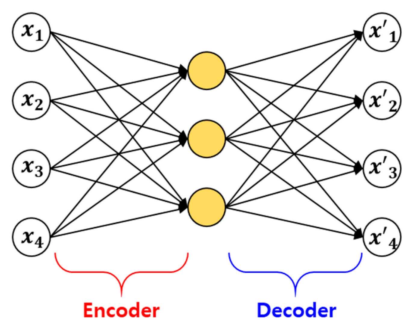
AutoEncoder is a type of ANN used to train efficient data codings in an unsupervised manner [17]. AutoEncoder simply copies input to output, as shown in Figure 6. The process seems simple, but it can have a variety of effects on data by constraining the network in different ways. Among them, Figure 6 shows a type of denoising AutoEncoder that reduces the number of neurons in the hidden layer to be smaller than that of the input layer, encodes the data to take only those characteristics, and then decodes it to remove noise.
In this study, the training efficiency of the learning model for ocean weather was maximized by passing data through the denoising AutoEncoder prior to training the data with the ConvLSTM and removing the noise. Of course, if we use the denoising AutoEncoder to remove the residual component (smoothing), the accuracy can be lowered. However, it is considered appropriate to use this method to solve the delay prediction problem using limited training data.

3. Deep Learning Model for the Prediction of Ocean Weather

As explained in Section 2.2 and Section 2.3, a deep learning model developed using the ConvLSTM and the denoising AutoEncoder is efficient in predicting eight parameters of ocean weather worldwide. This section describes the model used in this study to predict the actual ocean weather and the input data required to train the model.

3.1. Configuration of the Deep Learning Model

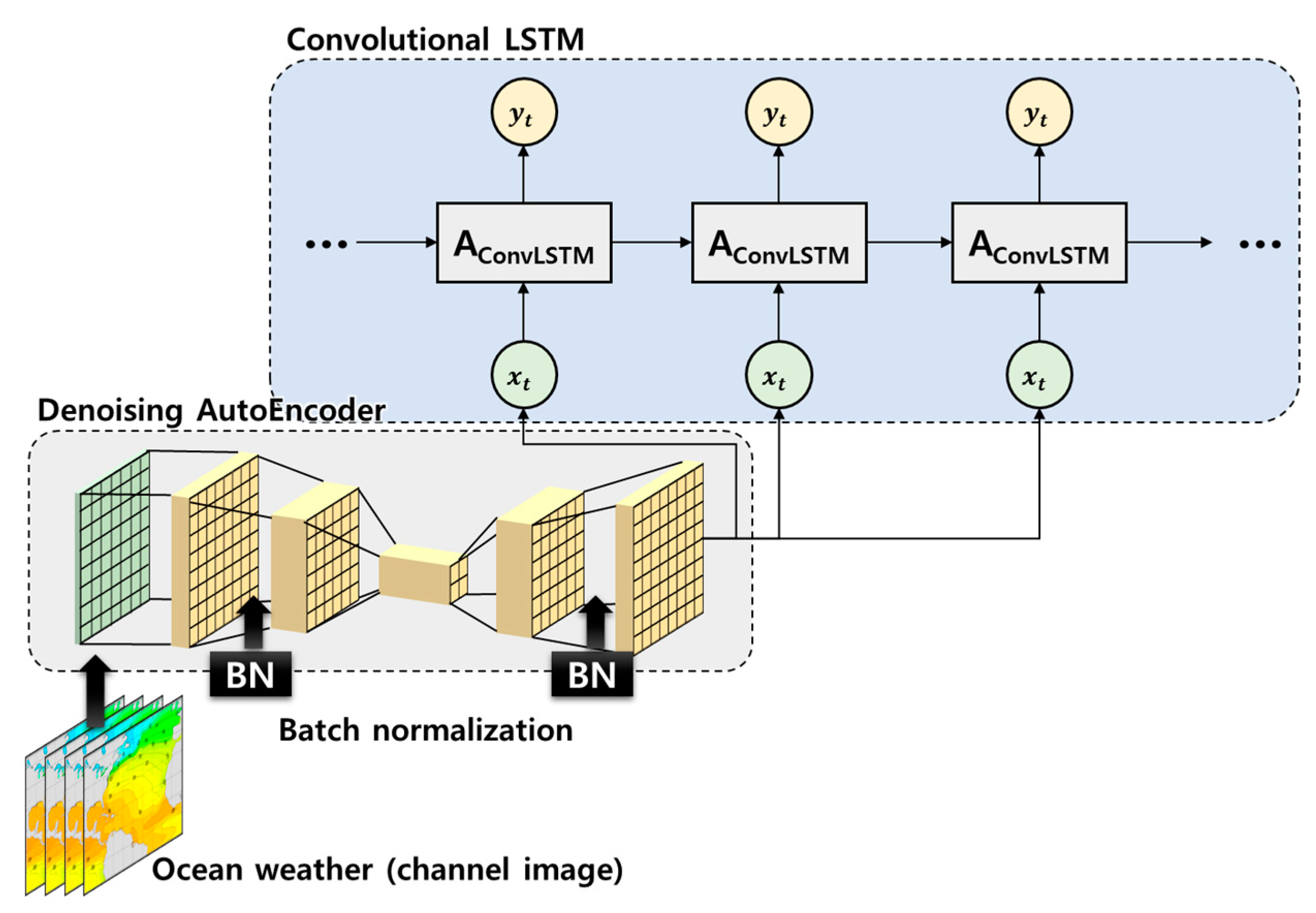
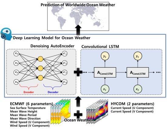
Figure 7 shows the configuration of the deep learning model proposed in this study. In this study, channel image data (set of 2D images of ocean weather) were used as input data. The noise of the input data was removed using the denoising AutoEncoder, and the input data from which noise was removed were used as input data for the ConvLSTM. The denoising AutoEncoder proposed in this study was trained as a single model in combination with the ConvLSTM. In the denoising AutoEncoder, as shown in Figure 7, two layers for encoding and two layers for decoding were used. In the two layers for encoding, the rectified linear unit (ReLU) was used as an activation function to prevent gradient vanishing, and in the two layers for decoding, the ReLU and the sigmoid were used as activation functions, respectively. At the end of the denoising AutoEncoder, the sigmoid was used to prevent the omission of data. At the end of the deep learning model, the sigmoid was also used as the activation function for the final output. In general, the ReLU, which is widely used as an activation function, treats all negative numbers as 0. If we use it as an activation function in the output layer, data loss may occur. However, the sigmoid function can output the value according to the scale of the input data; hence, the output data can be preserved as the scale of the input data. In addition, the adaptive moment estimation (ADAM) [18], which is well-known for its good performance, was used for weight optimization in all models. The input data comprised eight parameters of ocean weather, which were composed of several channels. When using data with multiple channels, there is an advantage that the causality between data composed of channels is considered. However, in the case of data that are not strongly correlated, learning models may produce undesirable effects. Therefore, in Section 3.3, the data that are useful to configure as a channel and use as a learning model are analyzed.
As shown in Figure 7, the channel image is first refined into the ConvLSTM through a denoising AutoEncoder. The denoising process is performed through the encoding layer of the second stage and the decoding layer of the second stage. When encoding and decoding are performed in the layer, a batch normalization step is additionally inserted to perform efficient denoising and prevent information escape. Batch normalization is a technique for improving the speed, performance, and stability of deep learning [19]. If the encoded image is used as an input to the ConvLSTM, the input data are entered in a compressed form; hence, the output trained through the ConvLSTM is not the same as the format of the input data. Therefore, the decoded image was used to make the input and output data the same. The denoised data are composed of data with the same dimensions as the initial input data and used as input for the ConvLSTM again. In this study, various ConvLSTM models were tested for ocean weather prediction, and their efficiency was analyzed. Details are discussed in Section 4.

3.2. Acquisition of Ocean Weather

In this study, eight parameters of publicly available ocean weather were accessed and used. Among them, six parameters (i.e., mean wave height (MWH), mean wave direction (MWD), mean wave period (MWP), wind speed (U component) (WU), wind speed (V component) (WV), and sea surface temperature (SST)) were accessed through the ECMWF. ERA-interim was used among the various models. ERA40 does not include data after 2002, and ERA5 includes more detailed information. However, it is not easy to download data for an extended period of time. Therefore, ERA-interim, which includes relatively accurate information over a long period of time, was used in this study. ERA-interim includes 6 h of data at intervals of 0.75 degrees in longitude and latitude. The data for 20 years (from October 1999 to September 2018) worldwide were gathered from ECMWF. Since information about current data is not included in ECMWF, the other two parameters of data (current speed (U component, simply, CU) and current speed (V component, simply, CV)) were accessed through the hybrid isopycnal–sigma–pressure coordinate ocean model (HYCOM). HYCOM provides three kinds of datasets: GLBy0.08, GLBu0.08, and GLBv0.08. GLBy0.08 does not include data before 2014, and GLBu0.08 includes data from 80S to 80N in latitude. In this study, we used the GLBv0.08 dataset, which includes long-term data and covers a large area of the 80S to 90N in latitude. GLBv0.08 includes 3 h of data at intervals of 0.08 degrees in longitude and latitude. The data accessed through HYCOM span a range of 4 years and 4 months (from July 2014 to November 2018) worldwide. For the route planning of a ship, it is necessary to forecast ocean weather from one week to a month. The captain does not change the route in real time during the voyage so that the route is re-determined every 12 h to a day. Therefore, 12 h of data is valid as a unit of time. In a spatial resolution, the denser intervals in longitude and latitude, the better. Generally, any resolution is linearly interpolated from nearby values. In this study, the eight parameters of ocean weather are composed of intervals of 6 h in time and of 1.5 degrees in longitude and latitude.
The raw data received from the ECMWF and HYCOM data servers are in .nc file format. The original data accessed in this study have very dense spacing. Therefore, we removed redundant data and used only the data necessary to train models, and the data were converted to .h5 file format using the h5py package. Through this process, the data to be used for the proposed model were generated.

3.3. Correlation Analysis of Ocean Weather

Eight parameters of ocean weather used in this study (SST, MWH, MWD, MWP, WU, WV, CU, and CV) not only have their own characteristics but also have correlated characteristics. For this reason, it is challenging to analyze and predict them. For example, in the case of SST, seasonal and trend components are very distinctive. On the other hand, MWD does not have a particular periodicity, and its prediction is difficult because the surrounding ocean weather profoundly influences it. As described in Section 2.3 and Section 3.1, we have to consider the spatial and correlation of each parameter of ocean weather. When considering the correlation of all eight parameters of data among each other, the input data may be composed of eight channels. However, training between data that lacks correlation decreases training efficiency. Therefore, in this study, we attempted to develop a learning model considering the correlation between each parameter of data.
Pearson’s correlation coefficient (PCC) [20], which is traditionally used in statistics, was used to analyze the correlations among the eight parameters of data. PCC is a numerical value quantifying the correlation between data X and Y. It has a value between +1 and −1, with a positive correlation for a positive value, a negative correlation for a negative value, and no correlation for a zero value. Generally, it is judged that there is a meaningful linear correlation with values of +0.5 or more or −0.5 or less.
Table 2 shows the absolute values of PCC for the eight parameters of data. For the calculation of PCC, one year of weather data in 2017 was used. The PCC results indicate that the wind speed (WU) and wave height (MWH) have a relatively high correlation compared to others, and the wave height and wave period (MWP) have a relatively high correlation. However, meaningful correlations, among other data, are difficult to find. The PCC can only analyze linear correlations. Therefore, considering that there will be a nonlinear correlation, we should review models that consider six ocean weather events at once. Among the input data obtained from ECMWF, SST, which does not correlate with other data, is employed as a single learning model, and the remaining five parameters of data are utilized as a single learning model. Finally, the two current-related data obtained from HYCOM are also used as a single learning model.

4. Applications

In this study, we attempted to determine the optimal learning model by testing various models. To find the optimal learning model for the eight parameters of data, we varied the input data period, forecasting point of the output data, and parameters of data to be tied to one learning model, and analyzed the results. The learning model was trained using a deep learning computer with the specifications indicated in Table 3. One computer was equipped with both CPU and GPU for the training.
With the computer of the specifications in Table 3, it takes about 3 s to predict the ocean weather for a time step. Therefore, it is judged that there will be no difficulty in predicting the ocean weather even with low-spec servers, and it is suitable to be used onboard.

4.1. Hyperparameters of the Learning Model

Hyperparameters for the ConvLSTM include the epoch number, batch size, and loss function type. Eight parameters of ocean weather were trained through a model combining the denoising AutoEncoder and the ConvLSTM. In the case of six parameters of ocean weather obtained from ECMWF, since it is a total of 20 years of data, the initial 16 years of data were used as a training set, and the remaining 4 years of data were used as a validation set (2 years) and a test set (2 years). In addition, in the case of two parameters of ocean weather obtained from HYCOM, since it is a total of 4 years and 4 months of data, the initial 4 years of data were used as a training set and the remaining 4 months of data were used as a validation set (2 months) and a test set (2 months). The batch size and number of epochs were tracked for the training set, validation set, and test set. The epoch number was determined using the convergence step from the line where no overfitting occurred. As a result of training progress, most models typically converge between 40 and 50 epochs. In this study, MAE was used in all cases for accuracy comparison. Since RMSE tends to overestimate outliers in the overall data, MAE is more appropriate for this study using time-series data for the long term. In the case of average error, the whole data are firstly calculated as MAE by comparing them with the original data and averaged. In addition, the land included in each area was also excluded from the error calculation. Due to the nature of the ConvLSTM, an image was used as an input, and the value of the land was calculated as 0. If the error of the land is included in the error, the total error will be smaller. In this study, we grasped this, calculated MAE for all areas and time series, and averaged it.

4.2. Effect of the Denoising AutoEncoder

The model described in Table 4 of Section 4.3 was trained using a model combining a denoising AutoEncoder and the ConvLSTM, as mentioned in Section 3.1. However, before that, we attempted to confirm the effect of the denoising AutoEncoder. For this, SST, which has a strong periodicity, was used. The results obtained using only the ConvLSTM model and those obtained using the denoising AutoEncoder and ConvLSTM models proposed in this study were compared.
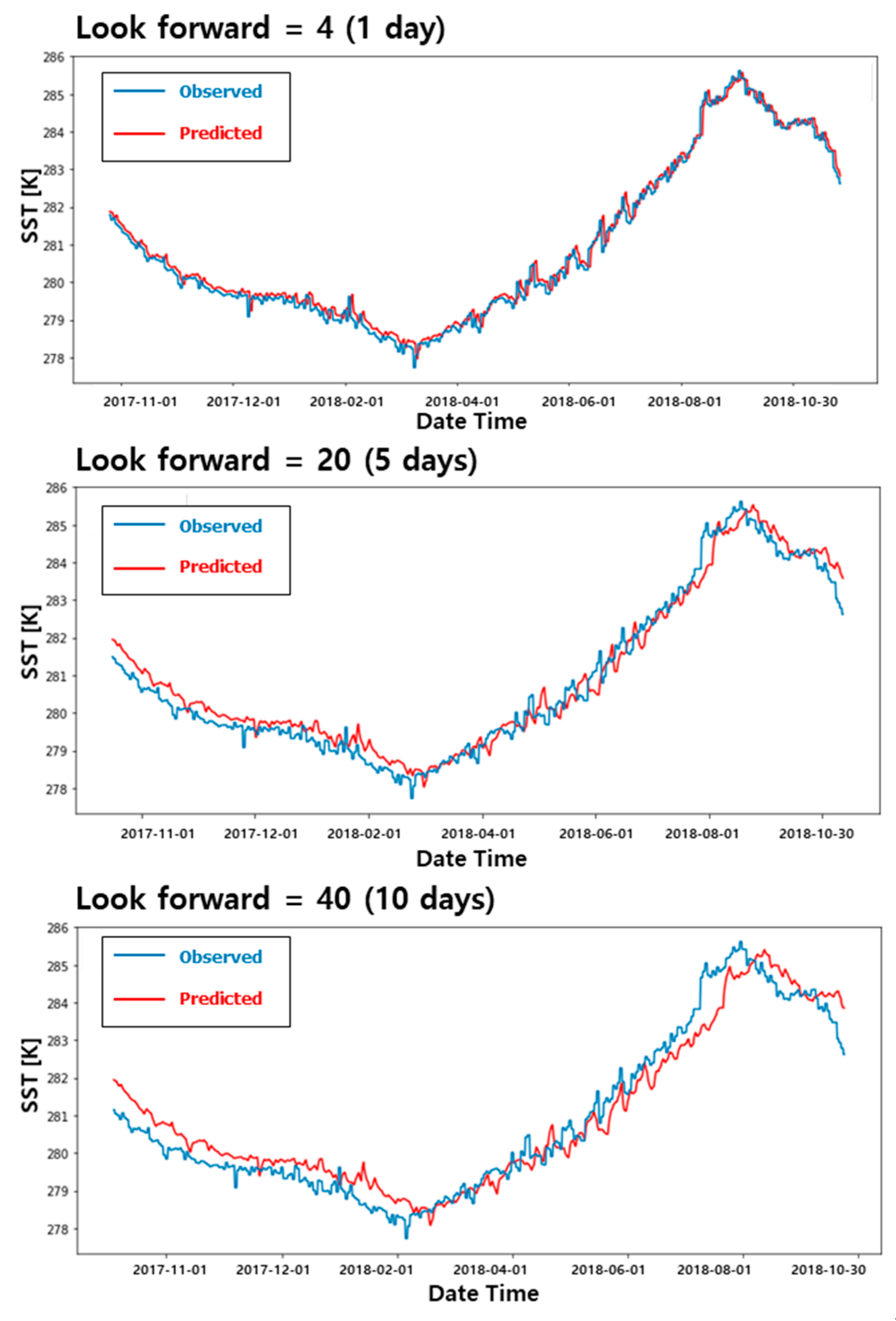
Prior to comparing the two models, to determine whether the delay prediction result occurs even when training SST, the look forward value was changed under the same conditions by using a single channel of SST as input data, and the accuracy was compared. Figure 8 shows the results of SST predictions for the Yellow Sea in South Korea for approximately a year in 2018. It shows the difference in prediction results according to the look forward value. When the look forward value was set to 4, 1 day later, a little difference was found between the observed value and the predicted value. However, evidently, the predicted value is similar to the shape when the observed value graph is slightly shifted to the right. When the look forward value is increased to 20 (5 days) and 40 (10 days), the delay prediction result can be clearly confirmed. Notably, the look forward value increases, and the delay prediction problem of the prediction result becomes more pronounced. This occurs because, as explained in Section 2.3, the learning model does not accurately grasp the data pattern because of the noise. As the look forward value increases, the farther the value to be predicted is from the current time when the prediction is made so that the current value can be scaled as it is and inferred as a prediction result. To address this problem, the noise should be removed by adding a denoising AutoEncoder to the ConvLSTM model.
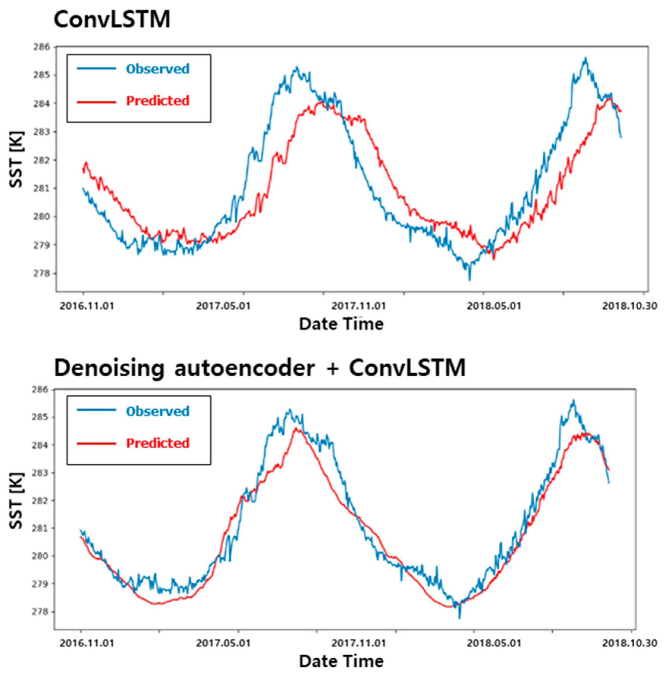
To analyze the effect of using the denoising AutoEncoder, SST of South Korea’s Yellow Sea was selected as a prediction target, as in the previous example. A total of 8 years of data were used, and a training set of 6 years and a test set of 2 years were used. The data were only used for this section and are different from the data mentioned in Section 4.1. Figure 9 shows the result of SST prediction. The upper graph is the prediction result using only the ConvLSTM, and the lower graph is the prediction result using the denoising AutoEncoder as the input of the ConvLSTM model. In the test case, models predicting a month (30 days) from the present were trained and compared whether the delayed problem is clearly visible or not. The result shows the last 2 years (from November 2016 to October 2018) of the predicted range, which was not used for training. The two data used in Figure 8 and Figure 9 are the same. However, in Figure 9, the graph was drawn using 2 years of data to show the effect of the denoising AutoEncoder clearly.
In Figure 9, the result using only the ConvLSTM shows a significantly delayed predicted result, as in Figure 8. The average error of the test set is 0.998 K, and when converted at a ratio according to the maximum and minimum value, it has an error of 10.97%. For the model using an additional denoising AutoEncoder, the delay prediction is clearly resolved. The average error of the test set is 0.474 K, showing an error of 5.26%. This is a 53% reduction in error compared with learning using the ConvLSTM alone, and as mentioned, the delay prediction problem has been solved. Therefore, in this study, a model combining a denoising AutoEncoder and the ConvLSTM was used to predict ocean weather.

4.3. Description of the Learning Models for Worldwide Data

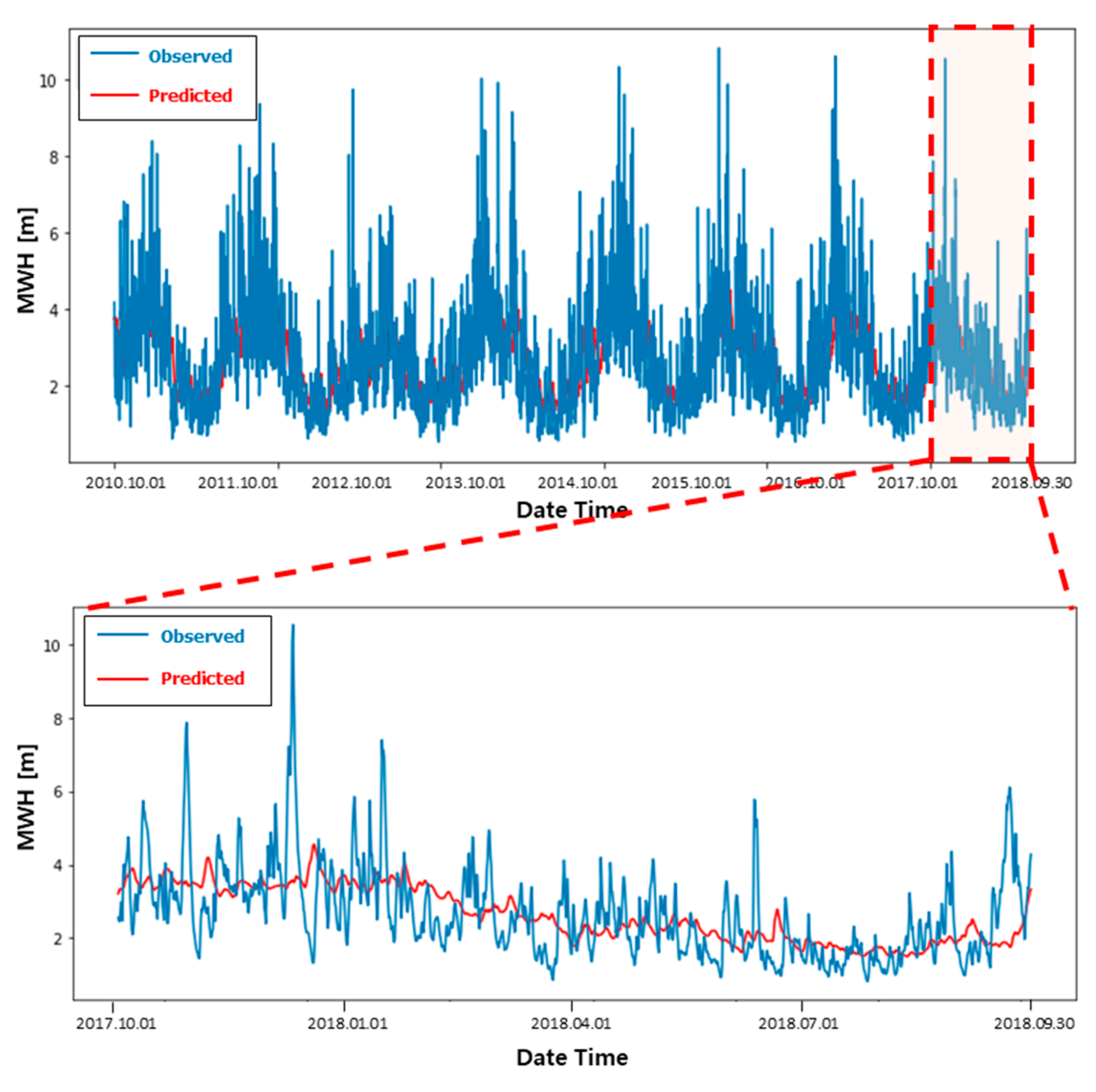
The disadvantage of not using the ConvLSTM described in Section 2.2 is that the characteristics of space and correlation between each parameter of ocean weather cannot be considered for learning. In addition, when using a conventional LSTM, an LSTM learning model must be created for each point where the prediction of ocean weather is desired. Figure 10 predicts MWH using the ConvLSTM. A total of 8 years of data were used for learning, 6 years were used as a training set, 1 year was used as a validation set, and the last 1 year was used as a test set. A model for predicting MWH after 7 days was trained using a total of 30 days of data. The batch size was 128, the number of hidden layers was 1, and the total number of nodes in the hidden layer was 32. The study was performed for 40 epochs until the model converged sufficiently. The lower graph in Figure 10 is an enlarged prediction result of the test set. The MAE of the test set was predicted relatively accurately at 0.78 m (4.8% error).
The conventional models of deep learning, such as DFN and LSTM, use data for specific locations to learn. Therefore, it is challenging to compare the ConvLSTM to DFN or LSTM directly. A large number of learning models are required to target worldwide data. Although the total number of models differs depending on how the resolution of the training model is set, 64,800 (= 180 × 360) models are needed worldwide to build a learning model for the ocean weather with resolutions of 1 degree in longitude and latitude. The recent increase in computing power has accelerated learning speed, but it takes considerable time to train 64,800 models. Therefore, in this study, the world was divided into 12 areas, and the proposed learning model was applied. Figure 11 shows the 12 areas used in this study. Dividing the latitude from −67.5° to 67.5° into three equal parts and the longitude from −180° to 180° into four equal parts divided the world into 12 equal pieces.
The structure of the learning model is important. However, setting the input, output, and hyperparameters of the learning model has a significant influence also in the learning efficiency. Therefore, this study attempted to analyze its effects through case studies of various input and output changes. A total of 240, 90, and 84 input data (look back) were used. Since the time interval of the ocean weather is 6 h, if there are 240 input data, this indicates that 60 days of data are used as input. In the case of ocean weather, trends over time should be considered. Therefore, if possible, it is good to have a long look back period. However, lengthening the look back period infinitely is impossible because there are limitations on the computation power of memory. In this manner, we used six hours of data. Therefore, assuming 90 steps as a look back, and it means using 22.5 days of data as input. However, when the interval of data is set to 1 day, a total of 90 days of data can be used as a look back. The accuracy, according to the interval of the ocean weather, was also analyzed.
In the case of output data (look forward), it denotes at which point the ocean weather is predicted through the look back data. In general, as the prediction time interval from the input data decreases, the accuracy increases. For example, predicting 1 day after the present is more accurate than predicting 1 week later. In this study, the accuracy was analyzed by changing the look forward to 4, 8, 12, and 28 steps. The look forward is similar to the look back. If the data interval is 6 h, 4 steps means a day later. Similarly, if the weather data are on a daily basis, 4 steps means 4 days later. In addition, in the case of look forward, shifting prediction is possible.
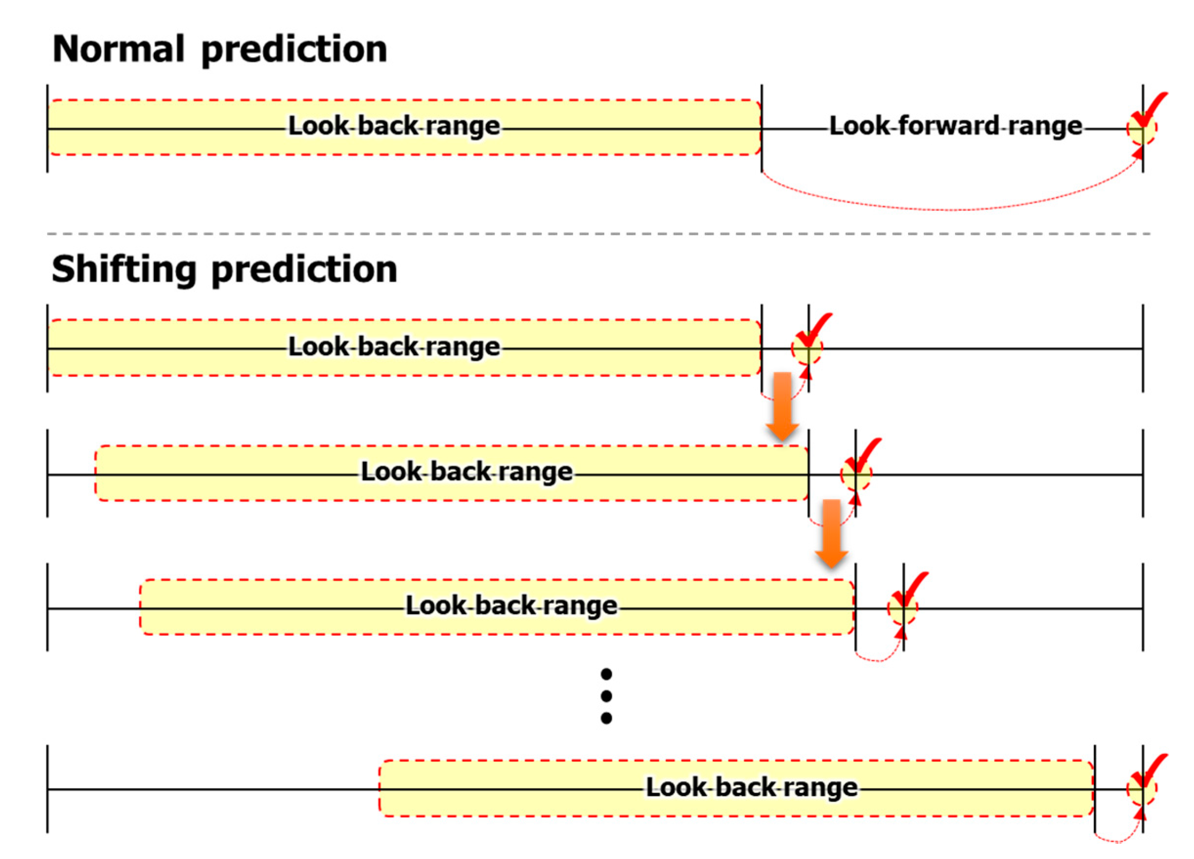
The shifting prediction is a method of predicting a specific point and using the predicted data as an input to predict the following continuously. For example, if the learning model is trained as a model that predicts one step forward, it cannot predict after four steps. In this case, the result of predicting the first step forward can be used as input again to predict the second step forward. By repeating this process, we can predict 4 steps forward and even can predict 100 steps forward. Figure 12 shows a comparison between normal prediction and shifting prediction. In the process of using deep learning models, we confirmed various studies on shifting prediction. Rasp et al. [21] performed a similar approach and named it “iterative prediction”. If the satellite communication is lost, we cannot get nowcasting information. However, we can predict any days in the future from past data by generating our own prediction model. In addition, using shifting forecasting allows for predicting the far future as well; thus, we can make a long-term plan. In this study, the difference in accuracy between the two methods was analyzed.
As explained earlier, it takes a lot of time and effort to train models by dividing the world into 12 areas. Therefore, it is necessary to find the appropriate number of input data to shorten the training time and to achieve affordable prediction accuracy. The original data are in intervals of 6 h. However, by adjusting it to an interval of one day, we compared the accuracy of making predictions using data from a longer period as a look back. Finally, as explained in Section 3.3, we compared and analyzed whether it is accurate to predict eight parameters of data with a single model and to divide the model through correlation analysis.
Table 4 shows the types of models trained in this study for comparison. Case 1 shows how much look back range could be accepted for the performance of the computer used in this study. Cases 3, 4, 5, 6, and 7 were compared to analyze the accuracy of the prediction model as the look forward increased. When predicting the same time, Cases 6 and 8 were used to determine whether it is correct to predict the time right or to make a shifting prediction. By comparing Cases 7 and 9, when predicting the same time, it was confirmed whether the prediction accuracy is maintained even if the number of data points for prediction is reduced. In Case 8, six channels (SST, MWH, MWP, MWD, WU, and WV) constituted a single learning model. In Case 9, a total of two models was trained. One is a prediction model that includes only one channel (SST), and the other is a prediction model that includes five channels (MWH, MWP, MWD, WU, and WV) to consider the correlation of each channel. The last two cases were selected to see which one was more accurate.
For accurate verification, K fold cross-validation is generally used, and training is performed commonly through a total of 10 fold cross-validation [22]. However, since the model of this study takes about one week for training each model, it is difficult to perform all cross-validation at the laboratory level. Due to this limitation, the cross-validation was not implemented here.

4.4. Case Studies and Discussion

All accuracy for case studies was measured using “Area 4” out of the 12 areas shown in Figure 11. The training time for computing varies depending on the look back range and the channel, but on average, it took approximately a week to train one model. Table 5 shows the accuracy of 11 cases. Accuracy was covered for all areas, including land. Since the training was performed with the image data, some data that are not on the land, such as SST or MWH, are assumed to be 0, and an image is generated and used as input.
In general, as the look back range increases, so does the prediction accuracy. However, the longer the look back range, the more memory allocation is required exponentially to train the models. If it is assumed to train the model for one area, the input data becomes an image of ocean weather during the look back range. Following the look back range, the number of images required for training increased significantly. In addition, if we use images of multiple channels, the number of images required for training is multiplied by the number of channels. If a multi-channel image is used as the input for the model using the lock back range of Case 1, training is impossible due to a memory problem. That is, if training is performed with the computing specifications in Table 3, training will not progress because of insufficient memory. Due to the limitation of computing power, it was determined that one channel was the maximum look back range for 240 steps in this study. In the case of Case 1, because training was performed with one channel of SST, there was not an insufficient memory issue. However, when training is conducted through one channel, the causality between each type of data cannot be considered. Therefore, to proceed with training in multiple channels, the look back range was reduced from the maximum allowed by the memory.
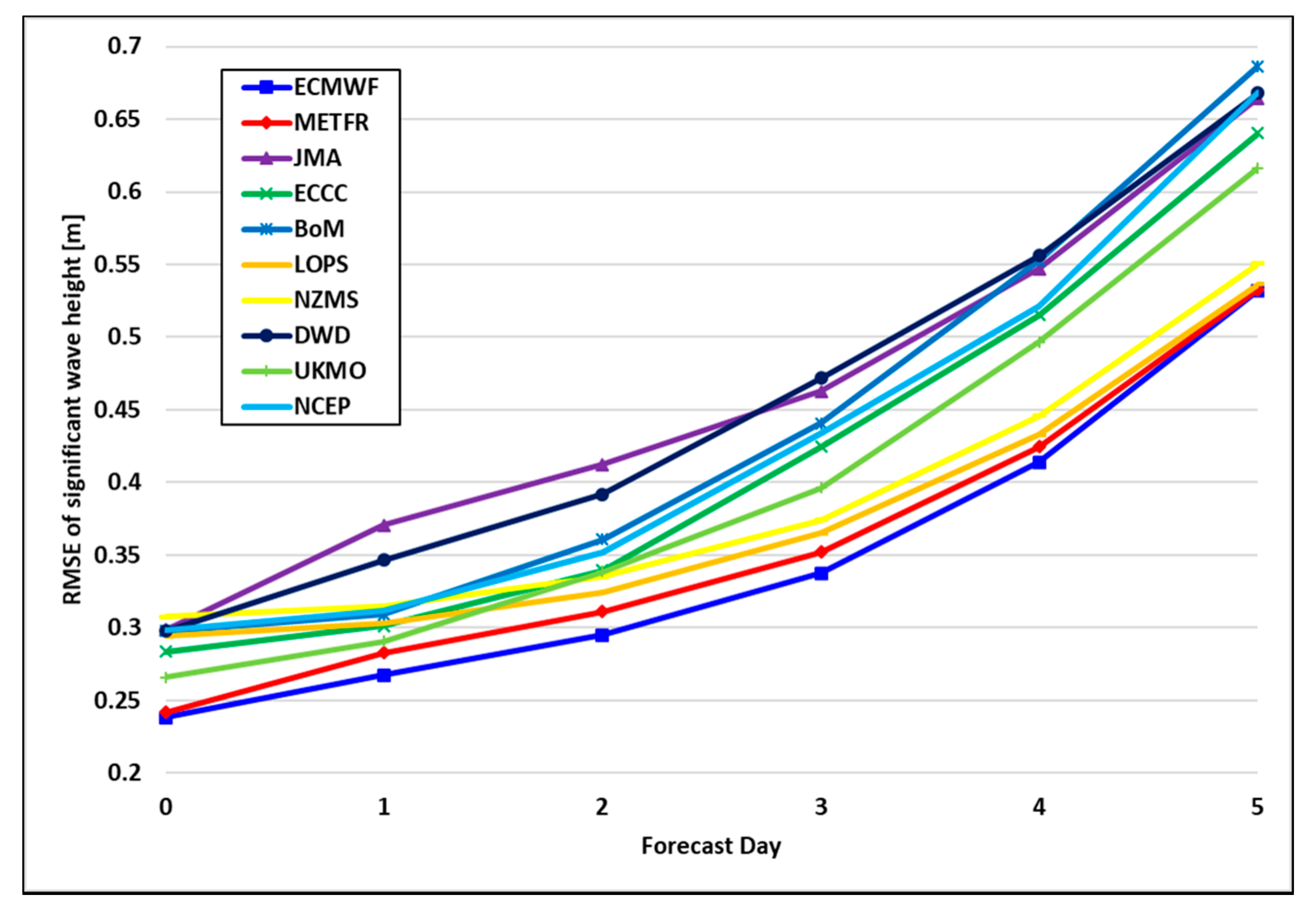
Cases 3–7 set the look back range to 22.5 days (90 steps) and performed training using six channels (SST, MWH, MWP, MWD, WU, and WV) of data. In Case 2, look forward was set to 6 h (1 step), and in Cases 4, 5, 6, and 7, training was performed after 1 day (4 steps), 2 days (8 steps), 3 days (12 steps), and 7 days (28 steps). When comparing the four cases, as the look forward increases, the prediction error also increases. The average errors of Cases 3–7 are 3.1%, 4.6%, 4.6%, 5.6%, and 5.1%, respectively. For accurate prediction, look forward should be small. However, the accuracy relatively remained over a range of look forward. In a typical prediction model for the ocean weather, the longer the forecast period, the higher the error, as shown in Figure 13. However, as the results presented in this study, it can be seen that the error does not increase after a certain period. Unlike the general prediction model based on physical phenomena, the deep learning-based prediction model presented in this study is a data-driven prediction model. Therefore, even if the prediction period is lengthened, the error does not increase indefinitely by considering the periodic and seasonal characteristics of the data at the same time.
When the same time was predicted in Cases 6 and 8, we determined whether the normal prediction or the shifting prediction was more accurate. As shown in Figure 12, shifting prediction is a method of predicting the next time point using the predicted data as input again and can easily predict the far future, regardless of the size of the look forward. Therefore, in this study, the accuracy of the two methods was compared through Cases 6 and 8. In Case 5, the look forward was set to 3 days (12 steps), and in Case 7, the result was predicted after 3 days by shifting; the model trained to predict after 6 h (1 step) was used. Cases 3 and 8 are the same learning model, but the error is much more significant when shifting prediction is performed. Case 5 showed an average error of 5.6%, but Case 7 showed a relatively high error of 10.0% because of the accumulation of errors during shifting. In Case 2, the SST and MWD errors were relatively high compared with the other data types. Since the errors accumulate and become more significant during shifting, in Case 7, SST and MWD are 23.1% and 18.3%, respectively, and the error was significantly increased compared with the other data types. By comparing the results of Cases 6 and 8, it can be observed that when predicting a relatively far future, it is more accurate to train the model as a normal prediction model than as a learning model for shifting prediction.
When the data at the same time were predicted in Cases 8 and 9, the data intervals used in the two models were different. Cases 8 and 9 used an interval of 1 day (originally, 4 steps). In this way, even if the same look forward was used, there was an advantage that prediction could be performed considering a longer period (longer look back range). Case 6 was a model that predicted 7 days later (look forward was 28 steps) using 22.5 days of data (look back range was 90). In Case 8, the look back range was also 90. However, because the interval of the data used for training was one, it was a model that predicts 7 days later using data from 90 days. Case 6 had an average error of 5.1%. In Case 8, the average error was 5.6%. When using the same look back range, it is more accurate to have a dense data interval. However, the difference in the error was not as large as it was in other comparisons.
In Cases 8 and 9, two models were compared in terms of accuracy. One was a learning model that consists of six channels of data in ECMWF, and the other one was a learning model where SST and five other parameters of data were divided into two models, as described in Section 3.3. The error of Case 8 was 5.6%, and the error of Case 9 was similar to that of Case 6, with an error of 5.1%. By comparing Cases 8 and 9, it was confirmed that it is more accurate to separate the model considering the causality. Therefore, this study consists of three models for predicting ocean weather. One was a single model of SST, and one was for the five remaining ECMWF data (MWH, MWP, MWD, WU, and WV). The last one was a model for HYCOM data (CU and CV).
Actually, it is hard to directly compare the accuracy of the model in this study with that of the general prediction model provided by weather centers. To compare the accuracy between them, the ocean weather data up to now should be obtained, and the proposed model should be generated using those data. However, ECMWF and HYCOM provide only data from several months ago; hence, it is difficult to obtain the data for generating the model at a specific point in time. In addition, even for predictions at a specific point in the past, they only provide actual data from the past, not data of how they predicted the weather at that time (i.e., past forecast data).
However, for indirect comparison, three parameters of verification data for the ocean weather (significant wave height (SWH), peak wave period (PWP), and wind speed (WS)) provided by the Weather Meteorological Organization (WMO) and ECMWF (2020) were additionally investigated. According to the verification data, it can be seen that the error rate accumulates and increases as the forecast period increases in the prediction models of weather centers. A total of ten organizations surveyed by the WMO compared the result of error between predicted ocean weather after three days and the actual value. The error of SWH is about 0.3–0.5 m, PWP is about 2.0–2.6 s, and WS is about 2.7–3.4 m/s, respectively. Figure 13 shows the RMSE of SWH presented in WMO and ECMWF [23]. In this study, the results of predicting the ocean weather after three days using the proposed model were presented in Section 4.4 (Case 5). As a result of predicting the ocean weather after three days using the proposed method in Case 5, the error was 0.22 m for MWH, 0.48 s for MWP, 2.46 m/s for WU, and 2.24 m/s for WV, respectively. It can be seen that it shows a similar error rate presented by WMO and ECMWF (2020). Therefore, if there is no experience to make a numerical prediction model for the ocean weather, the proposed method is expected to be helpful.

4.5. Prediction Results of Worldwide Ocean Weather

We proposed a learning model for predicting ocean weather using the ConvLSTM model and denoising AutoEncoder. In addition, through the case studies in Section 4.4, the accuracy of the learning models according to various look back and look forward ranges was compared and analyzed. Based on the comparison, the model used in Case 9 was applied to training the models worldwide. As described in Section 3.2, the eight parameters of data used in this study consist of data that have 6-h intervals and spatial intervals of 0.75° in longitude and latitude. If the 0.75° interval data are used for one region shown in Figure 11, an image size of 120 × 30 pixels should be applied. This induced practical difficulty in training because of the specifications of Table 3 in terms of memory. Therefore, data were organized at intervals of 1.5° in longitude and latitude. Finally, training was performed using an image of 60 × 30 pixels per area.
In addition, as described in Section 4.4, three models per area in the 12 areas were used for prediction, and 36 prediction models were used to predict the ocean weather worldwide. In the case of look back, 84 days of data (12 weeks) was used, and a model for predicting after 7 days was constructed. Table 6 shows the prediction accuracy for the eight parameters of ocean weather in the 12 areas.
In Table 6, the area with the lowest error is shown in blue, and the area with the highest error is shown in red, for each parameter of ocean weather. In addition, the area with the lowest average error was marked with blue shade, and the area with the highest error was marked with a red shade. The average error for the eight parameters of data worldwide was 6.7%, and the results were quite different in each area, ranging from 4.1% to 9.7%. When comparing the error rates for each area, it can be seen that Areas 1, 3, 4, and 6 have higher average errors than the other areas. This is because it is challenging to consider spatial influences in learning because the land is included in these areas. However, in Areas 10 and 11, the error rate is significantly higher than in other areas, even though these areas contain little land. This is because, despite the fact that the area includes a large ocean area, the ocean weather varied so much that the learning model could not grasp the pattern correctly.
By analyzing the error rate for each type of data, the error rate of the current is significantly lower than that of the other types. In this study, the HYCOM data were used for training the CU and CV, and the data range was relatively short (4.4 years data) compared with the ECMWF data. However, the error rate was low compared with the other types of data. It was expected to be easy for the learning model to grasp the pattern because the current is relatively small, and there is little change compared with the other data. Conversely, in the case of MWD, the error rate was significantly higher than that of other data, which may have occurred because the fluctuation range is very severe and there is no periodicity relative to the other types of data.
5. Conclusions and Future Works

As explained in Section 1, there is a demand for shipping companies and classification societies to make a solution for predicting ocean weather on their own, which is currently only provided through weather centers. However, they were inexperienced in building a long-term, data-driven numerical model. Therefore, this study proposed a data-driven learning model for solving the lack of experience. In this study, we proposed a deep learning model that combines a denoising AutoEncoder and the ConvLSTM to predict ocean weather. With the ConvLSTM, we can train a model that predicts ocean weather over a wide range of regions by taking advantage of 2D data. That is, we can train the model over a wide area at once and consider the causality between points in the area. In addition, using data with noise removed by the denoising AutoEncoder as input, the problem of delay prediction, which frequently occurs when training time-series data, was solved. The method proposed in this study can be regarded as an initial study for the solutions to be provided for shipping companies or classification societies. In the case of the method of the ocean weather forecasting to be used in real solutions, the higher the accuracy, the better. However, currently, we are developing under the judgment that it is available if it has an error rate of around 5%.
Through a variety of case studies, first, a model capable of training on the computer used in this study was selected. Second, analyzing the results of the learning model when changing the look back range, it was confirmed that as the look back range increased, the results were more accurate. It was expected that the prediction accuracy would decrease as the look forward increased. However, as a result of the prediction, it was confirmed that there was an exponential relationship, and the average error value converged to a value between 5 and 5.5. In addition, the results seemed to have an exponential relationship with the look forward value and the accuracy of the model, and it will be identified through further research. When comparing the predictions of the normal prediction and the shifting predictions, it was confirmed that the model that predicts a specific time point at once was more accurate than the shifting model when predicting the far future. It was confirmed that the accuracy was similar when the intervals of input data were varied to use the longer periodicity as input. Finally, it was determined that it is more accurate to build a model by dividing the model according to causality, rather than predicting all data as a single model.
In this study, the world was divided into 12 areas to construct the worldwide learning model, and three learning models were trained for each area. The model proposed in this study was found to have satisfactory accuracy, with an average error of 6.7%. Although this study is in an early stage and the accuracy is not yet excellent enough to be commercially available, it has confirmed the possibility of applying the data-driven method to predict ocean weather worldwide. The goal of this study is to develop further and expand the proposed method to provide a more accurate and reliable forecast service for ocean weather.
When using the learning model, it was found that there is still some room for improvement. In order to obtain the ocean weather at the beginning of the study, it was confirmed that NOAA, ECMWF, and HYCOM provided the ocean weather. Among them, ECMWF and HYCOM were accessed and used in this study. In the future, we will search for various providers and upgrade the input data to be used. As mentioned in Section 4.4, because of the lack of memory, the look back range was selected as 12 weeks. In the future, we intend to build more accurate models by increasing the look back range using a computer with better performance. In addition, currently, the land existed in 2D images was used as input data. In this case, for data types such as SST and MWH, if the value is not on the land, it was assigned a value of 0. In the ConvLSTM, which considers spatial relationships, this can adversely affect accuracy. Therefore, there is an additional need for a method to manage the influence of land on the input data in the future. Ocean weather has significant features for each region. Therefore, in order to build good learning models, it is necessary to divide it into areas with similar characteristics, such as the North Sea, the Atlantic Ocean, and the Pacific Ocean. Probably considering these characteristics, it is expected that we can build models that are superior to the error rate suggested in this study. In addition, we plan to carry out a sensitivity test for shifting prediction and to verify the proposed model with the climatology. Therefore, we plan to improve the models by reflecting the point of view in the future.

Author Contributions

Conceptualization, K.-S.K., J.-B.L., and M.-I.R.; methodology, K.-S.K., J.-B.L., and M.-I.R.; software, K.-S.K. and J.-B.L.; validation, K.-S.K., J.-B.L., and M.-I.R.; formal analysis, K.-S.K., J.-B.L., and M.-I.R.; investigation, K.-S.K., J.-B.L., and M.-I.R.; resources, M.-I.R.; data curation K.-S.K. and J.-B.L.; writing—original draft preparation, K.-S.K.; writing—review and editing, M.-I.R.; visualization, K.-S.K.; supervision, M.-I.R.; project administration, M.-I.R.; funding acquisition, M.-I.R., K.-M.H., and G.-H.L. All authors have read and agreed to the published version of the manuscript.

Funding

This work was partially supported by (a) Korean Register, Republic of Korea, (b) HRD Program for Green & Smart Ship funded by the Ministry of Trade, Industry and Energy, Republic of Korea (No. P0001968), (c) Research Institute of Marine Systems Engineering of Seoul National University, Republic of Korea, and (d) Institute of Engineering Research of Seoul National University, Republic of Korea.

Conflicts of Interest

The authors declare no conflict of interest. The funders had no role in the design of the study; in the collection, analyses, or interpretation of data; in the writing of the manuscript, or in the decision to publish the results.

References

  1. ISO. ISO 15016:2015-Ships and Marine Technology-Guidelines for the Assessment of Speed and Power Performance by Analysis of Speed Trial Data; ISO: Geneva, Switzerland, 2015. [Google Scholar]
  2. Gunaydin, K. The estimation of monthly mean significant wave heights by using artificial neural network and regression methods. Ocean Eng. 2008, 35, 1406–1415. [Google Scholar] [CrossRef]
  3. James, S.C.; Zhang, Y.; Donncha, F.O. A machine learning framework to forecast wave conditions. Coast. Eng. 2018, 137, 1–10. [Google Scholar] [CrossRef] [Green Version]
  4. Jain, P.; Deo, M.C. Artificial intelligence tools to forecast ocean waves in real time. Open Ocean Eng. J. 2008, 13–20. [Google Scholar] [CrossRef] [Green Version]
  5. Mahjoobi, J.; Kazeminezhad, M.H. Hindcasting of wave parameters using different soft computing methods. Appl. Ocean Res. 2008, 30, 28–36. [Google Scholar] [CrossRef]
  6. Zhang, Q.; Wang, H.; Dong, J.; Zhong, G. Prediction of Sea Surface Temperature Using Long Short-Term Memory. IEEE Geosci. Remote Sens. Lett. 2017, 14, 1745–1749. [Google Scholar] [CrossRef] [Green Version]
  7. Cortes, C.; Vladmir, V. Support-vector networks. Mach. Learn. 1995, 20, 273–297. [Google Scholar] [CrossRef]
  8. Rumelhart, D.E.; Hinton, G.E.; Williams, R.J. Learning representations by back-propagating errors. Nature 1986, 323, 533–536. [Google Scholar] [CrossRef]
  9. Lim, B.; Zohren, S. Time series forecasting with deep learning: A survey. arXiv 2020, arXiv:2004.13408. [Google Scholar]
  10. Donahue, J.; Hendricks, L.A.; Rohrbach, M.; Venugopalan, S.; Guadarrama, S.; Saenko, K.; Darrell, T. Long-term recurrent convolutional networks for visual recognition and description. IEEE Trans. Pattern Anal. Mach. Intell. 2015, 39, 677–691. [Google Scholar] [CrossRef] [PubMed]
  11. Lecun, Y.; Bengio, Y.; Hinton, G. Deep learning. Nature 2015, 521, 436–444. [Google Scholar] [CrossRef] [PubMed]
  12. Shi, X.; Chen, Z.; Wang, H.; Yeung, D.-Y.; Wong, W.; Woo, W. Convolutional LSTM network: A machine learning approach for precipitation nowcasting. Adv. Neural Inf. Process. Syst. 2015, 802–810. [Google Scholar]
  13. Conway, A.J.; Macpherson, K.P.; Brown, J.C. Delayed time series predictions with neural networks. Neurocomputing 1998, 18, 81–89. [Google Scholar] [CrossRef]
  14. Deng, T.; Cheng, A.; Han, W.; Lin, H.X. Visibility forecast for airport operations by LSTM neural network. In Proceedings of the 11th International Conference on Agents and Artificial Intelligence, Prague, Czech Republic, 19–21 February 2019; Volume 2, pp. 466–473. [Google Scholar]
  15. Cleveland, R.B.; Cleveland, W.S.; McRae, J.E.; Terpenning, I. STL: A Seasonal-Trend decomposition Procedure Based on Loess. J. Off. Stat. 1990, 6, 3–73. [Google Scholar]
  16. Antonelli, P.; Tobin, D.; Revercomb, H.; Turner, D.; Dutcher, S.; Howell, B.; Knuteson, B.; Vinson, K.; Smith, W.L. Application of PCA to Hyperspectral Data for Noise Characterization, Noise Filtering and Instrument Monitoring. Available online: https://www.ecmwf.int/node/15617 (accessed on 14 October 2020).
  17. Kramer, M.A. Nonlinear principal component analysis using autoassociative neural networks. AIChE J. 1991, 37, 233–243. [Google Scholar] [CrossRef]
  18. Kingma, D.P.; Ba, J.L. Adam: A method for stochastic optimization. In Proceedings of the 3rd International Conference on Learning Representations, ICLR 2015—Conference Track Proceedings, San Diego, CA, USA, 7–9 May 2015; pp. 1–15. [Google Scholar]
  19. Ioffe, S.; Szegedy, C. Batch normalization: Accelerating deep network training by reducing internal covariate shift. In Proceedings of the 32nd International Conference on Machine Learning, ICML 2015, Lille, France, 6–11 July 2015; Volume 1, pp. 448–456. [Google Scholar]
  20. Pearson, K. Note on regression and inheritance in the case of two parents. In Proceedings of the Royal Society of London; Royal Society of London: London, UK, 1895; pp. 240–242. [Google Scholar]
  21. Rasp, S.; Dueben, P.D.; Scher, S.; Weyn, J.A.; Mouatadid, S.; Thuerey, N. WeatherBench: A benchmark dataset for data-driven weather forecasting. arXiv 2020, arXiv:2002.00469v3. [Google Scholar] [CrossRef]
  22. McLachlan, G.; Do, K.-A.; Ambroise, C. Analyzing Microarray Gene Expression Data; Wiley: New York, NY, USA, 2004. [Google Scholar]
  23. WMO; ECMWF. Intercomparison of Operational Wave Forecasting Systems against In-Situ Observations: Data from BoM, DMI, DWD, ECCC, ECMWF, JMA, LPOS, METEOAM, METFR, METNO, NCEP, NZMS, PRTOS, SHNSM, UKMO; WMO: Geneva, Switzerland; ECMWF: Reading, UK, 2020. [Google Scholar]
Figure 1. The necessity of self-prediction of the weather forecast.
Jmse 08 00805 g001
Figure 2. Configuration of long short-term memory (LSTM) and cell state “A”.
Jmse 08 00805 g002
Figure 3. Cell state configuration of the convolutional LSTM (ConvLSTM).
Jmse 08 00805 g003
Figure 4. The delayed prediction problem of sea surface temperature (SST).
Jmse 08 00805 g004
Figure 5. The decomposed components of SST from 2014 to 2017.
Jmse 08 00805 g005
Figure 6. Configuration of AutoEncoder for denoising.
Jmse 08 00805 g006
Figure 7. Configuration of the deep learning model for ocean weather.
Jmse 08 00805 g007
Figure 8. Results of predicting SST using the ConvLSTM according to look forward steps.
Jmse 08 00805 g008
Figure 9. Results of predicting SST using the ConvLSTM and denoising AutoEncoder.
Jmse 08 00805 g009
Figure 10. Results of predicting mean wave height (MWH) using conventional LSTM.
Jmse 08 00805 g010
Figure 11. The divided 12 areas for learning models.
Jmse 08 00805 g011
Figure 12. Comparison between normal prediction and shifting prediction.
Jmse 08 00805 g012
Figure 13. RMSE of significant wave height for ten organizations [23].
Jmse 08 00805 g013
Table 1. Summary of related works and this study.
StudyInput DataEstimation ObjectivesEstimation ModelsEstimation AreaEstimation Time Range
Jain et al. [4]Wave heightWave heightANN, GP, MTArabian Sea3 to 72 h
Mahjoobi et al. [5]Wind direction, wind speed, duration, fetch length Wave height, period, directionANN, ANFIS, FISLake OntarioPresent point
Gunaydin [2]Wind speed, sea level pressure, air temperatureWave heightANN (7 models)Atlantic OceanPresent point
Zhang et al. [6]SSTSSTLSTMCoastal seas near China1 day to 1 month
James et al. [3]Wave height, period, direction, wind speed, current speedWave height, periodMLP, SVMMonterey BayN/A
This studySST, wave height, wave period, wave direction, wind speed (U component), wind speed (V component), current speed (U component), current speed (V component)SST, wave height, wave period, wave direction, wind speed (U component), wind speed (V component), current speed (U component), current speed (V component)Convolutional LSTM + Denoising AutoEncoderWorldwide6 h to one week
Table 2. Pearson’s correlation coefficient for ocean weather.
Pearson’s Correlation CoefficientSSTWUWVMWHMWDMWPCUCV
SST1.000.240.190.360.320.390.310.32
WU-1.000.030.700.110.070.130.07
WV--1.000.040.150.020.030.12
MWH---1.000.020.680.320.11
MWD----1.000.250.270.13
MWP-----1.000.290.20
CU------1.000.31
CV-------1.00
Table 3. Computing specification for training deep learning model.
CategorySpecification
CPUIntel Xeon E5-2640 v4 (2.4 Ghz) × 2 EA
GPUGeForce RTX 2080 8 GB × 4 EA
RAMDDR4 32GB PC4-19200 (2400 MHz) × 4 EA = 128 GB
Table 4. Learning model configurations.
CasesInput Data RangeOutput DataChannel Configuration
(Look Back Steps)(Look Forward Steps)
Case 160 days (240)After 6 h (1)1 channel (SST)
Case 222.5 days (90)After 6 h (1)6 channels (SST, MWH, MWP, MWD, WU, WV)
Case 322.5 days (90)After 1day (4)6 channels (SST, MWH, MWP, MWD, WU, WV)
Case 422.5 days (90)After 2 days (8)6 channels (SST, MWH, MWP, MWD, WU, WV)
Case 522.5 days (90)After 3 days (12)6 channels (SST, MWH, MWP, MWD, WU, WV)
Case 622.5 days (90)After 7 days (28)6 channels (SST, MWH, MWP, MWD, WU, WV)
Case 722.5 days (90)After 3 days (1-shifting)6 channels (SST, MWH, MWP, MWD, WU, WV)
Case 890 days (90)After 7 days (7)6 channels (SST, MWH, MWP, MWD, WU, WV)
Case 984 days (84)After 7 days (7)1 channel (SST), 5 channels (MWH, MWP, MWD, WU, WV)
Table 5. Summary of estimation accuracy for all cases.
CasesSST Error [°K]MWH Error [m]MWP Error [s]MWD Error [deg]WU Error [m/s]WV Error [m/s]Average Error [%]
Case 11.84
(9.3%)
N/AN/AN/AN/AN/A9.3
Case 22.84
(9.3%)
0.09
(0.6%)
0.25
(1.4%)
11.21
(3.1%)
1.21
(2.0%)
1.19
(2.1%)
3.1
Case 33.31
(10.8%)
0.13
(0.8%)
0.32
(1.4%)
19.43
(5.3%)
1.80
(2.9%)
1.84
(3.2%)
4.1
Case 42.69
(8.8%)
0.18
(1.2%)
0.40
(2.3%)
28.34
(7.8%)
2.28
(3.7%)
2.24
(3.9%)
4.6
Case 53.68
(12.1%)
0.22
(1.5%)
0.48
(2.8%)
33.76
(9.3%)
2.46
(4.0%)
2.38
(4.1%)
5.6
Case 63.16
(10.4%)
0.18
(1.2%)
0.42
(2.4%)
32.15
(8.9%)
2.33
(3.8%)
2.24
(3.9%)
5.1
Case 77.03
(23.1%)
0.28
(1.8%)
0.95
(5.5%)
66.12
(18.3%)
3.41
(5.5%)
3.46
(5.6%)
10.0
Case 84.11
(13.5%)
0.17
(1.4%)
0.44
(2.5%)
32.66
(9.0%)
2.05
(3.4%)
1.99
(3.8%)
5.6
Case 93.47
(4.2%)
0.44
(3.5%)
0.75
(4.7%)
28.27
(7.8%)
3.06
(5.0%)
3.17
(5.2%)
5.1
Table 6. Summary of the prediction accuracy for all areas.
AreasSST Error [°K]MWH Error [m]MWP Error [s]MWD Error [deg]WU Error [m/s]WV Error [m/s]CU Error
[m/s]
CV Error
[m/s]
Average Error
Area 12.81
(7.8%)
0.82
(5.1%)
1.15
(6.4%)
57.20
(15.9%)
4.04
(5.5%)
4.64
(5.9%)
0.12
(4.0%)
0.12
(3.7%)
6.8%
Area 22.05
(5.2%)
0.74
(4.4%)
1.10
(6.4%)
72.77
(20.2%)
6.01
(4.0%)
4.49
(4.3%)
0.12
(2.5%)
0.11
(2.3%)
6.2%
Area 33.74
(9.7%)
0.46
(3.7%)
0.88
(5.3%)
71.84
(20.0%)
3.56
(5.7%)
3.76
(6.4%)
0.09
(3.0%)
0.09
(3.0%)
7.1%
Area 43.47
(9.9%)
0.74
(4.6%)
1.07
(6.1%)
77.08
(21.4%)
20.18
(7.9%)
4.56
(3.6%)
0.15
(3.5%)
0.15
(3.1%)
7.5%
Area 53.70
(9.8%)
0.36
(4.6%)
1.13
(6.8%)
52.25
(14.5%)
2.03
(4.1%)
2.22
(3.6%)
0.13
(2.9%)
0.12
(3.2%)
6.2%
Area 63.40
(9.9%)
0.82
(5.5%)
1.84
(11.0%)
72.42
(20.1%)
3.33
(4.9%)
3.03
(4.9%)
0.14
(3.7%)
0.13
(3.5%)
7.9%
Area 71.63
(4.6%)
0.58
(6.2%)
1.42
(8.4%)
39.11
(10.9%)
3.54
(7.3%)
3.75
(6.5%)
0.15
(3.0%)
0.14
(3.0%)
6.2%
Area 81.08
(3.0%)
0.34
(3.1%)
0.82
(4.8%)
29.29
(8.1%)
2.21
(4.2%)
2.00
(3.2%)
0.13
(3.0%)
0.12
(3.1%)
4.1%
Area 91.34
(4.0%)
0.85
(6.0%)
1.17
(7.0%)
43.32
(12.0%)
4.80
(8.0%)
5.00
(7.8%)
0.12
(4.1%)
0.12
(4.2%)
6.6%
Area 102.38
(8.9%)
1.09
(11.6%)
1.76
(10.7%)
77.47
(21.5%)
5.47
(10.3%)
5.21
(9.1%)
0.13
(2.9%)
0.13
(2.9%)
9.7%
Area 112.92
(9.2%)
0.93
(6.2%)
1.36
(8.0%)
37.68
(10.5%)
5.00
(7.6%)
7.96
(9.9%)
0.15
(3.0%)
0.15
(2.6%)
7.1%
Area 121.07
(3.1%)
0.81
(5.4%)
1.10
(6.5%)
31.40
(8.7%)
4.52
(6.9%)
4.71
(6.3%)
0.13
(2.9%)
0.13
(3.1%)
5.4%
Average error2.47
(7.1%)
0.71
(5.5%)
1.23
(7.3%)
55.15
(15.3%)
5.39
(6.4%)
4.28
(6.0%)
0.13
(3.2%)
0.13
(3.2%)
6.7%
Publisher’s Note: MDPI stays neutral with regard to jurisdictional claims in published maps and institutional affiliations.