Local Scour for Vertical Piles in Steady Currents: Review of Mechanisms, Influencing Factors and Empirical Equations

Abstract
1. Introduction
2. Influencing Factors
2.1. Intensity of Flow
2.2. Flow Depth
2.3. Sediments
2.4. Pile
2.5. Time
2.5.1. Finite Time
2.5.2. According to Asymptotically Functions
2.5.3. According to Critical Shear Stress
3. Empirical Equations
3.1. Exponential Formulas
3.2. Logarithmic Formulas
3.3. Hyperbolic Functions
3.4. Numerical Functions
4. Conclusions
- (1)
- A local scour around a vertical pile involves interactions between sediments and flow fields, which is a process with complicated three-dimensional turbulence. Down-flow in front of a pile and the existed incoming boundary layer are essential in forming the horseshoe vortex. Shear stress at the pile edges, which are produced by the concentrated streamlines, will be amplified to a range of 5–10 times compared to that of the approach flow. Due to this amplification, scour was found to start at the pile upstream corners. Interactions between the three-dimensional horseshoe vortex and vortices shedding are responsible for scour behind the pile.
- (2)
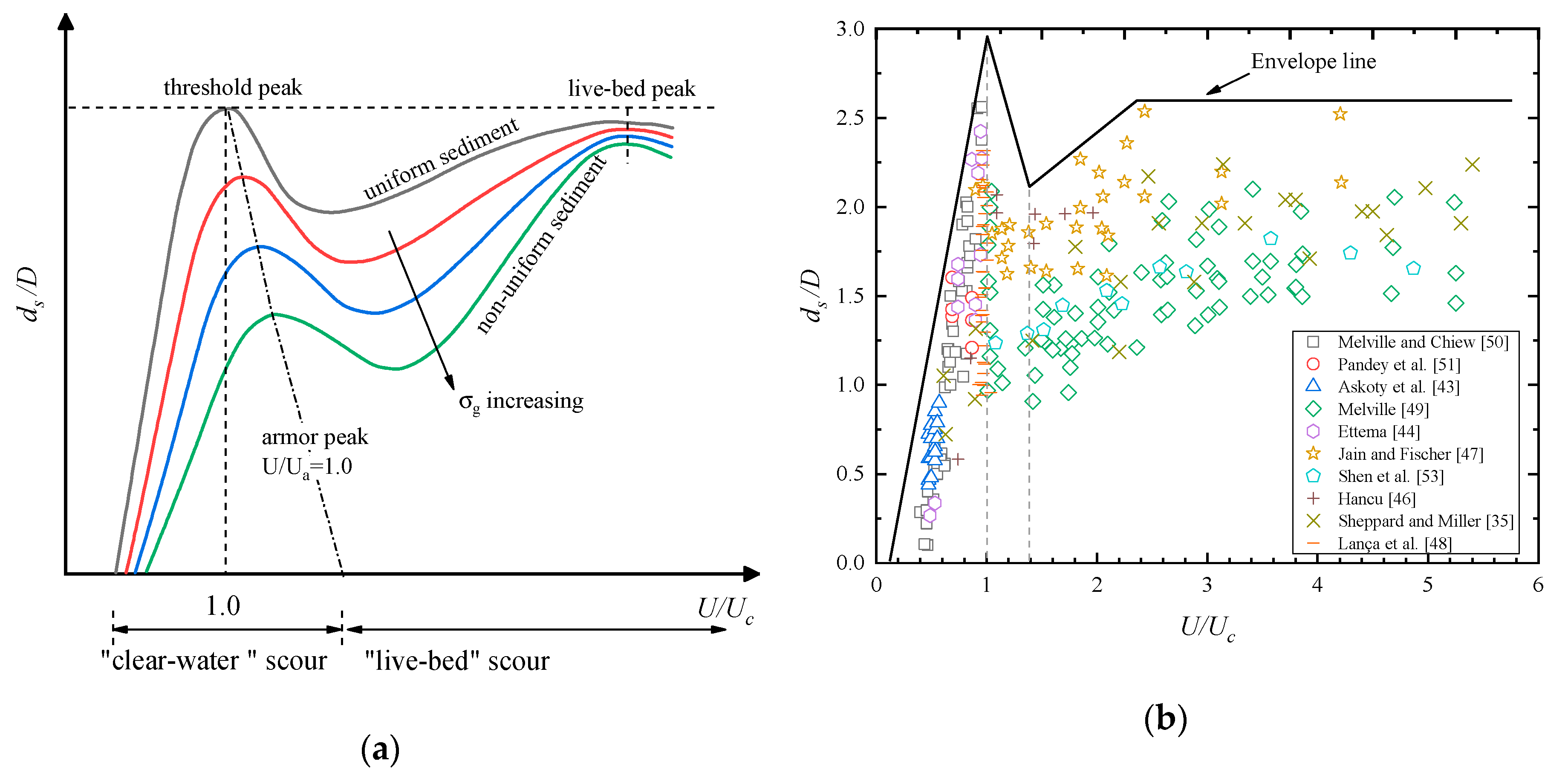
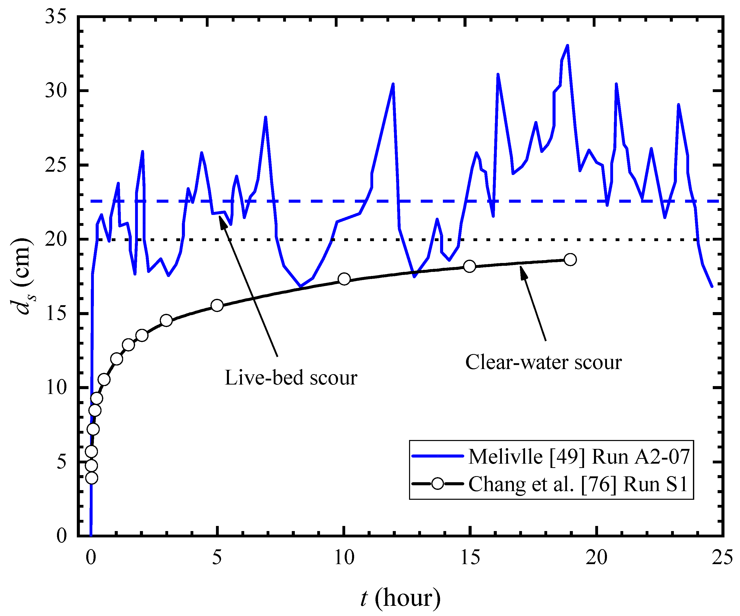
- The flow intensity in uniform sediments or non-uniform sediments connects the approach flow velocity and sediment particles. In clear-water scour conditions, flow intensity is smaller than 1. Maximum scour depths were found at the transition from clear-water scour to live-bed scour conditions. The existing equilibriums of local scour in clear-water scour conditions indicated that shear stress in scour hole was smaller than the critical shear stress of sediment particle. In live-bed scour conditions, due to the supplements of sediments particles from upstream, equilibrium scour depth oscillates near the mean value. Both uniform and non-uniform sediments attained to their second scour depth peaks when the flow intensity was about 4.0.
- (3)
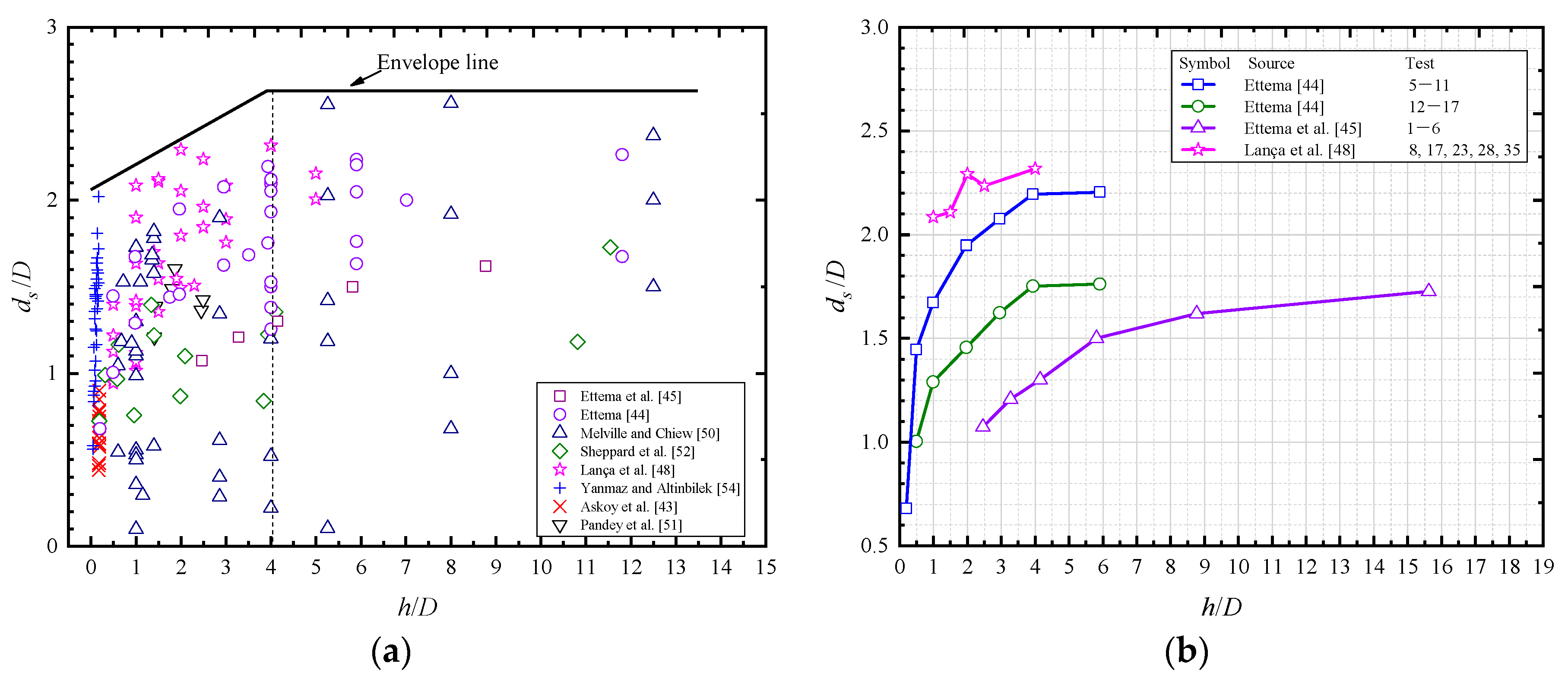
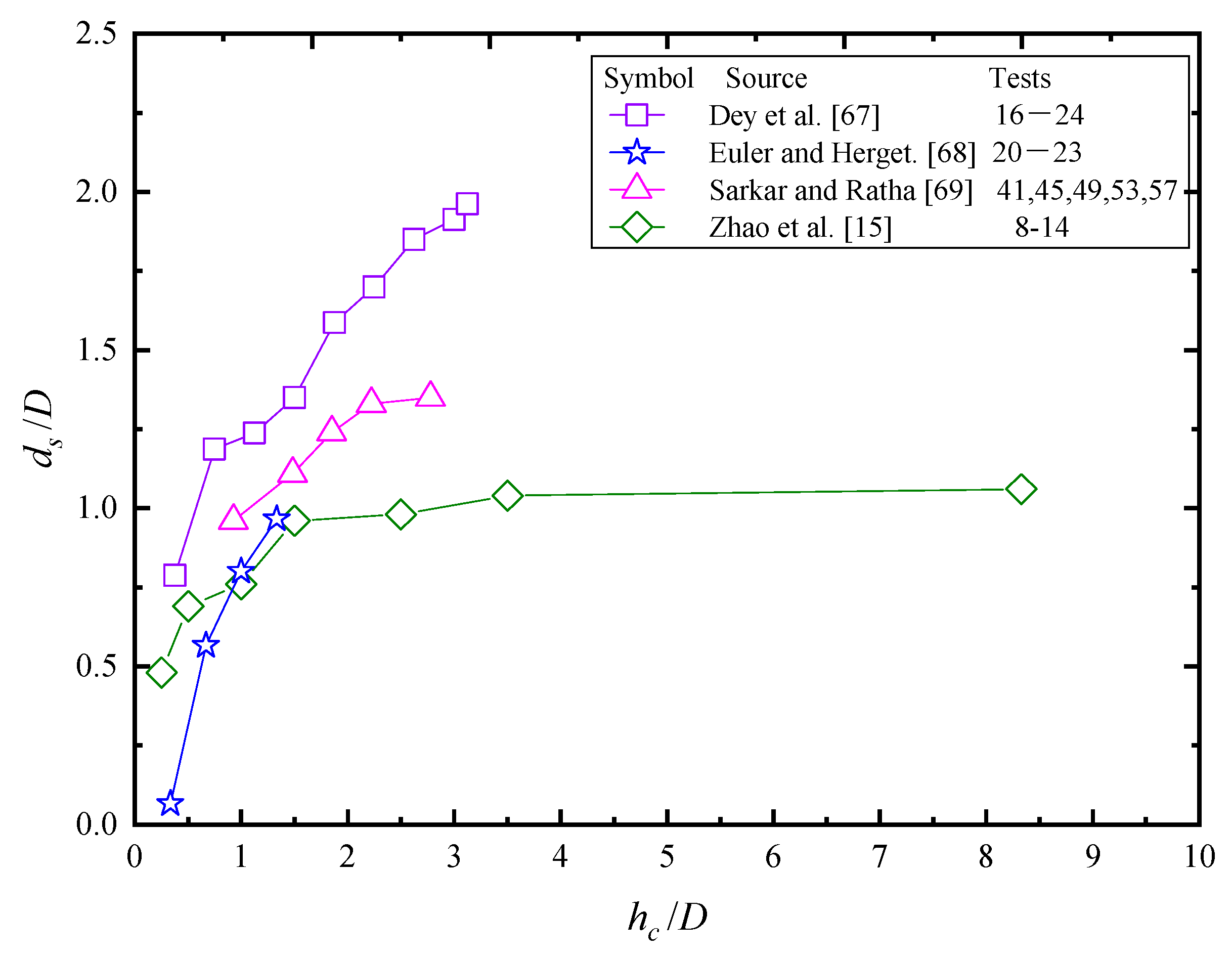
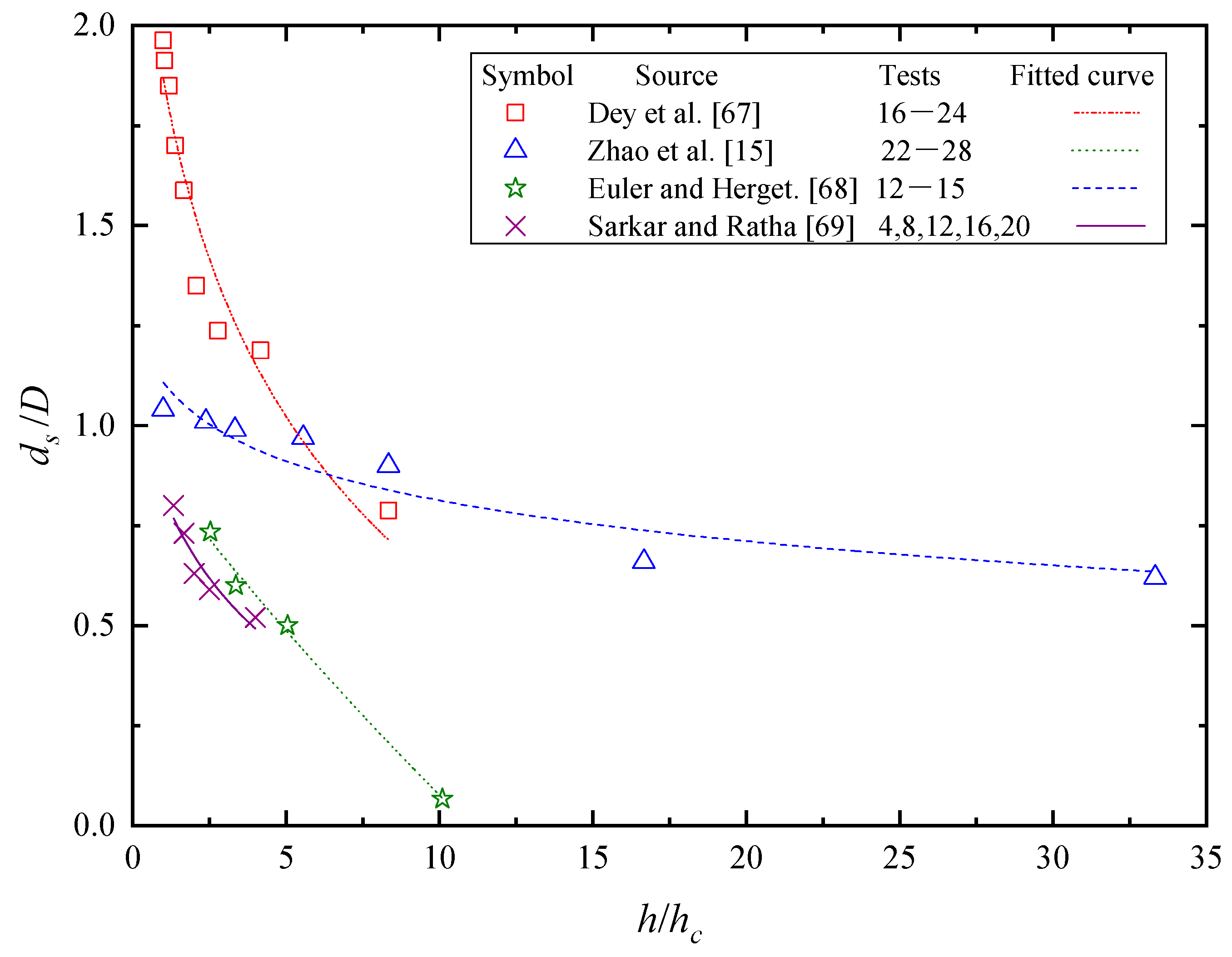
- Flow depth is an important factor in local scour. The unsubmerged vertical piles have been studied far more than that of submerged cases. In unsubmerged conditions, the maximum scour depth increased with the increasing flow depth until to a critical value. A curve (Figure 3a), which enveloped large amounts of experimental data, could give a reference in scour depth design when considering the flow depth effects. Due to the different flow fields, more studies are needed in submerged cases such as caissons, manifolds in offshore engineering.
- (4)
- Sediments parameters of medium size and non-uniformity in local scour were connected with flow intensity. Armoring effects, which decreased scour depth in non-uniform sediments, were found to increase with the increasing sediments gradation. However, reviews and conclusions in this paper were only for non-cohesive sediments.
- (5)
- Scour depth increases with pile width and pile height. In submerged cases, relative scour depth decreases with the increasing submergence ratio . For live-bed scour conditions, the relative scour depth tends to be a constant value when the submergence ratio surpasses 2.
- (6)
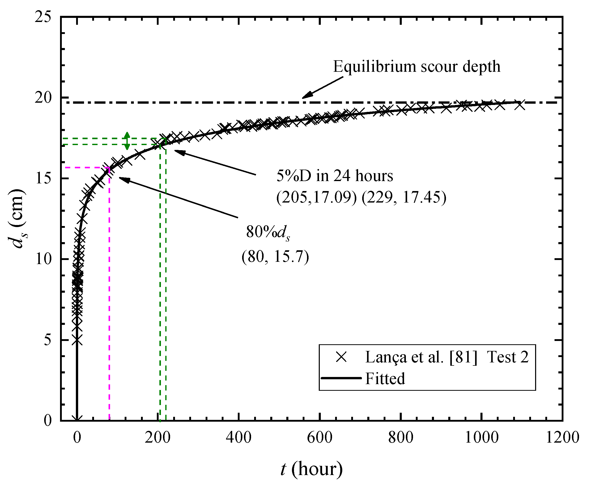
- Certifications for equilibrium of scour depth used by researchers vary broadly. Categories of finite time, according to asymptotically functions and according to the shear stress in scour hole were classified. Different equations based on these certifications with experimental data have been adopted in literature. Empirical equations were categorized into four types: exponential formula, logarithmic formula, hyperbolic functions and numerical functions.
Author Contributions
Funding
Acknowledgments
Conflicts of Interest
References
- Hunt, J.C.R.; Abell, C.J.; Peterka, J.A.; Woo, H. Kinematical studies of the flows around free or surface-mounted obstacles: Applying topology to flow visualization. J. Fluid Mech. 1978, 86, 179–200. [Google Scholar] [CrossRef]
- Liu, K.; Liu, J.L.; Yu, W.C. Statistical Analysis of Bridges Caused by Floods from 2007 to 2015. Urban Roads Bridges Flood Control 2017, 1, 90–92. [Google Scholar]
- Ettema, R. Scour at Bridge Piers; Report No. 216; University of Auckland: Auckland, New Zealand, 2016. [Google Scholar]
- Zhao, M.; Zhu, X.; Cheng, L.; Teng, B. Experimental study of local scour around subsea caissons in steady currents. Coast. Eng. 2012, 60, 30–40. [Google Scholar] [CrossRef]
- Chabert, J.; Engeldinger, P. Etude des Affouillements Autour des Piles des Ponts; Laboratoire National d’Hydraulique: Chatou, France, 1956. [Google Scholar]
- Roulund, A.; Sumer, B.M.; Fredsøe, J.; Michelsen, J. Numerical and experimental investigation of flow and scour around a circular pile. J. Fluid Mech. 2005, 534, 351–401. [Google Scholar] [CrossRef]
- Keshavarzi, A.; Melville, B.; Ball, J. Three-dimensional analysis of coherent turbulent flow structure around a single circular bridge pier. Environ. Fluid Mech. 2004, 14, 821–847. [Google Scholar] [CrossRef]
- Okamoto, S.; Sunabashiri, Y. Vortex shedding from a circular cylinder of finite length placed on a ground plane. J. Fluids Eng. 1992, 114, 512–521. [Google Scholar] [CrossRef]
- Pattenden, R.J.; Turnock, S.R.; Zhang, X. Measurements of the flow over a low-aspect-ratio cylinder mounted on a ground plane. Exp. Fluids 2005, 39, 10–21. [Google Scholar] [CrossRef]
- Baker, C.J. The laminar horseshoe vortex. J. Fluid Mech. 1979, 95, 344–367. [Google Scholar] [CrossRef]
- Hjorth, P. Studies on the Nature of Local Scour. Ph.D. Thesis, Department of Water Resources Engineering, Lund Institute of Technology, University of Lund, Scania, Sweden, 1975. [Google Scholar]
- Guan, D.W.; Chiew, Y.M.; Wei, M.X.; Hsieh, S.C. Characterization of horseshoe vortex in a developing scour hole at a cylindrical bridge pier. Int. J. Sediment Res. 2019, 34, 118–124. [Google Scholar] [CrossRef]
- Mattioli, M.; Alsina, J.M.; Mancinelli, A.; Miozzi, M.; Brocchini, M. Experimental investigation of the nearbed dynamics around a submarine pipeline laying on different types of seabed: The interaction between turbulent structures and particles. Adv. Water Resour. 2012, 48, 31–46. [Google Scholar] [CrossRef]
- Sumer, B.M.; Fredsøe, J. The Mechanics of Scour in the Marine Environment, 4th ed.; World Scientific: Singapore, 2002; pp. 149–228. [Google Scholar]
- Zhao, M.; Cheng, L.; Zang, Z. Experimental and numerical investigation of local scour around a submerged vertical circular cylinder in steady currents. Coast. Eng. 2010, 57, 709–721. [Google Scholar] [CrossRef]
- Manes, C.; Brocchini, M. Local scour around structures and the phenomenology of turbulence. J. Fluid Mech. 2015, 779, 309–324. [Google Scholar] [CrossRef]
- Unger, J.; Hager, W. Down-flow and horseshoe vortex characteristics of sediment embedded bridge piers. Exp. Fluids 2007, 42, 1–19. [Google Scholar] [CrossRef]
- Kirkil, G.; Constantinescu, G.; Ettema, R. Coherent structures in the flow field around a circular cylinder with scour hole. J. Hydraul. Eng. 2008, 134, 572–587. [Google Scholar] [CrossRef]
- Kolmogorov, A.N. The local structure of turbulence in incompressible viscous fluid for very large Reynolds numbers. Proc. R. Soc. Lond. Ser. A: Math. Phys. Sci. 1991, 434, 9–13. [Google Scholar] [CrossRef]
- Frisch, U. Turbulence: The Legacy of A. N. Kolmogorov; Cambridge University Press: New York, NY, USA, 1995; 296p. [Google Scholar]
- Li, J.; Qi, M.; Fuhrman, D.R.; Chen, Q. Influence of turbulent horseshoe vortex and associated bed shear stress on sediment transport in front of a cylinder. Exp. Therm. Fluid Sci. 2018, 97, 444–457. [Google Scholar] [CrossRef]
- Tseng, M.H.; Yen, C.L.; Song, C.C.S. Computation of three-dimensional flow around square and circular piers. Int. J. Numer. Methods Fluids. 2000, 34, 207–227. [Google Scholar] [CrossRef]
- Dargahi, B. The turbulent flow field around a circular cylinder. Exp. Fluids 1989, 8, 1–12. [Google Scholar] [CrossRef]
- Kobayashi, T.; Oda, K. Experimental study on developing process of local scour around a vertical cylinder. In Proceedings of the 24th International Conference on Coastal Engineering, Kobe, Japan, 23–28 October 1994; Volume 93, pp. 1284–1297. [Google Scholar]
- Sumer, B.M.; Fredsøe, J.; Christiansen, N. Scour around vertical pile in waves. J. Waterw. Port Coast. Ocean Eng. 1992, 118, 15–31. [Google Scholar] [CrossRef]
- Sumer, B.M.; Christiansen, N.; Fredsøe, J. The horseshoe vortex and vortex shedding around a vertical wall-mounted cylinder exposed to waves. J. Fluid Mech. 1997, 332, 41–70. [Google Scholar] [CrossRef]
- Rudolph, D.; Bos, K.J. Scour around a monopile under combined wave current conditions and low KC-numbers. In Proceedings of the Third International Conference on Scour and Erosion, Amsterdam, The Netherlands, 1–3 November 2006; pp. 582–588. [Google Scholar]
- Qi, W.G.; Gao, F.P. Physical modeling of local scour development around a large diameter monopile in combined waves and current. Coast. Eng. 2014, 83, 72–81. [Google Scholar] [CrossRef]
- Zanke, U.C.E.; Hsu, T.W.; Roland, A.; Link, O.; Diab, R. Equilibrium scour depths around piles in noncohesive sediments under currents and waves. Coast. Eng. 2011, 58, 986–991. [Google Scholar] [CrossRef]
- Miozzi, M.; Corvaro, S.; Pereira, F.A.; Brocchini, M. Wave-induced morphodynamics and sediment transport around a slender vertical cylinder. Adv. Water Resour. 2019, 129, 263–280. [Google Scholar] [CrossRef]
- Sumer, B.M.; Petersen, T.U.; Locatelli, L.; Fredsøe, J.; Musumeci, R.E.; Foti, E. Backfilling of a scour hole around a pile in waves and current. J. Waterw. Port Coast. Ocean Eng. 2013, 139, 9–23. [Google Scholar] [CrossRef]
- Agudo, J.R.; Luzi, G.; Han, J.; Hwang, M.; Lee, J.; Wierschem, A. Detection of particle motion using image processing with particular emphasis on rolling motion. Rev. Sci. Instrum. 2017, 88, 051805. [Google Scholar] [CrossRef] [PubMed]
- Dey, S.; Ali, S.Z. Stochastic mechanics of loose boundary particle transport in turbulent flow. Phys. Fluids 2017, 29, 055103. [Google Scholar] [CrossRef]
- Mia, F.; Nago, H. Design method of time-dependent local scour at circular bridge pier. J. Hydraul. Eng. 2003, 129, 420–427. [Google Scholar] [CrossRef]
- Sheppard, D.M.; Miller, W. Live-bed local pier scour experiments. J. Hydraul. Eng. 2006, 132, 635–642. [Google Scholar] [CrossRef]
- Chiew, Y.M.; Melville, B.W. Local scour around bridge piers. J. Hydraul. Res. 1987, 25, 15–26. [Google Scholar] [CrossRef]
- Guo, J.K. Semi-analytical model for temporal clear-water scour at prototype piers. J. Hydraul. Res. 2014, 52, 366–374. [Google Scholar] [CrossRef]
- Kothyari, U.C.; Hager, W.H.; Oliveto, G. Generalized approach for clear-water scour at bridge foundation elements. J. Hydraul. Eng. 2007, 133, 1229–1240. [Google Scholar] [CrossRef]
- Cheng, N.S.; Chiew, Y.M.; Chen, X.W. Scaling Analysis of Pier-Scouring Processes. J. Eng. Mech. 2016, 142, 06016005. [Google Scholar] [CrossRef]
- Yanmaz, A.M. Temporal variation of clear-water scour at cylindrical bridge piers. Can. J. Civ. Eng. 2006, 33, 1098–1102. [Google Scholar] [CrossRef]
- Melville, B.M.; Sutherland, A.J. Design method for local scour at bridge piers. J. Hydraul. Eng. 1988, 114, 1210–1226. [Google Scholar] [CrossRef]
- Baykal, C.; Sumer, B.M.; Fuhrman, D.R.; Jacobsen, N.G.; Fredsøe, J. Numerical investigation of flow and scour around a vertical circular cylinder. Philos. Trans. R. Soc. A Math. Phys. Eng. Sci. 2015, 373, 20140104. [Google Scholar] [CrossRef] [PubMed]
- Aksoy, A.O.; Bombar, G.; Arkis, T.; Guney, M.S. Study of the time-dependent clear water scour around circular bridge piers. J. Hydrol. Hydromech. 2017, 65, 26–34. [Google Scholar] [CrossRef]
- Melville, B. The physics of local scour at bridge piers. In Proceedings of the Fourth International Conference on Scour and Erosion, Tokyo, Japan, 5–7 November 2008; pp. 228–238. [Google Scholar]
- Ettema, R. Scour at Bridge Piers. Ph.D. Thesis, University of Auckland, Auckland, New Zealand, 1980. [Google Scholar]
- Ettema, R.; Kirkil, G.; Muste, M. Similitude of large-scale turbulence in experiments on local scour at cylinders. J. Hydraul. Eng. 2006, 132, 33–40. [Google Scholar] [CrossRef]
- Hancu, S. Sur le calcul des affouillements locaux dans la zone des piles des ponts. In Proceedings of the 14th AHR Congress International Association for Hydro Research (IAHR), Paris, France, 29 August–3 September 1971; Volume 3, pp. 299–313. [Google Scholar]
- Jain, S.C.; Fischer, E.E. Scour around Bridge Piers at High Froude Numbers; Report No. FH-WA-RD-79-104; Federal Highway Administration: Washington, DC, USA, 1979. [Google Scholar]
- Lança, R.M.; Fael, C.S.; Maia, R.J.; Pêgo, J.P.; Cardoso, A.H. Clear-water scour at comparatively large cylindrical piers. J. Hydraul. Eng. 2013, 139, 1117–1125. [Google Scholar] [CrossRef]
- Melville, B.W. Live-bed scour at bridge sites. J. Hydraul. Eng. 1984, 110, 1234–1247. [Google Scholar] [CrossRef]
- Melville, B.W.; Chiew, Y.M. Time scale for local scour at bridge piers. J. Hydraul. Eng. 1999, 125, 59–65. [Google Scholar] [CrossRef]
- Pandey, M.; Sharma, P.K.; Ahmad, Z.; Karna, N. Maximum scour depth around bridge pier in gravel bed streams. Nat. Hazards 2018, 91, 819–836. [Google Scholar] [CrossRef]
- Sheppard, D.M.; Odeh MGlasser, T. Large scale clear-water local pier scour experiments. J. Hydraul. Eng. 2004, 130, 957–963. [Google Scholar] [CrossRef]
- Shen, H.W.; Schneider, V.R.; Karaki, S.S. Mechanics of Local Scour. National Bureau of Standards; Institute of Applied Technology, U.S. Department of Commerce: Washington, DC, USA, 1966. [Google Scholar]
- Yanmaz, M.; Altinbilek, H.D. Study of time-dependent local scour around bridge piers. J. Hydraul. Eng. 1991, 117, 1247–1268. [Google Scholar] [CrossRef]
- Baker, C.J. The position of points of maximum and minimum shear stress upstream of cylinders mounted normal to flat plates. J. Wind Eng. Ind. Aerodyn. 1985, 18, 263–274. [Google Scholar] [CrossRef]
- Raudkivi, A.J.; Ettema, R. Clear-water scour at cylindrical piers. J. Hydraul. Eng. 1983, 131, 338–350. [Google Scholar] [CrossRef]
- Park, C.W.; Park, H.I.; Cho, Y.K. Evaluation of the applicability of pier local scour formulae using laboratory and field data. Mar. Georesour. Geotechnol. 2017, 35, 1–7. [Google Scholar] [CrossRef]
- Dey, S. Three-dimensional vortex flow field around a circular cylinder in a quasi-equilibrium scour hole. Sādhanā 1995, 12, 771–785. [Google Scholar] [CrossRef]
- Hoffmans, G.J.C.M.; Verheij, H.J. Scour Manual, A.A, 2nd ed.; Balkema: Rotterdam, The Netherlands, 1997; 205p. [Google Scholar]
- Oliveto, G.; Hager, W.H. Temporal evolution of clear-water pier and abutment scour. J. Hydraul. Eng. 2002, 128, 811–820. [Google Scholar] [CrossRef]
- Chiew, Y.M.; Melville, B.W. Local scour at bridge piers with non-uniform sediments. Proceedings of the institution of civil engineers. Publ. Telford Ltd. 1989, 87, 215–224. [Google Scholar]
- Mir, B.H.; Lone, M.A.; Bhat, J.A.; Rather, N.A. Effect of Gradation of Bed Material on Local Scour Depth. Geotech. Geol. Eng. 2018, 36, 2505–2516. [Google Scholar] [CrossRef]
- Melville, B.W. Pier and abutment scour: Integrated approach. J. Hydraul. Eng. 1997, 123, 125–136. [Google Scholar] [CrossRef]
- Lee, S.O.; Sturm, T.W. Effect of sediment size scaling on physical modeling of bridge pier scour. J. Hydraul. Eng. 2009, 135, 793–802. [Google Scholar] [CrossRef]
- Sarkar, K.; Chakraborty, C.; Mazumder, B.S. Variations of bed elevations due to turbulence around submerged cylinder in sand beds. Environ. Fluid Mech. 2016, 16, 659–693. [Google Scholar] [CrossRef]
- Dey, S.; Raikar, R.; Roy, A. Scour at Submerged Cylindrical Obstacles under Steady Flow. J. Hydraul. Eng. 2008, 134, 105–109. [Google Scholar] [CrossRef]
- Euler, T.; Herget, J. Obstacle-Reynolds-number based analysis of local scour at submerged cylinders. J. Hydraul. Res. 2011, 49, 267–271. [Google Scholar] [CrossRef]
- Sarkar, A.; Ratha, D. Flow around submerged structures subjected to shallow submergence over plane bed. J. Fluids Struct. 2014, 44, 166–181. [Google Scholar] [CrossRef]
- Tsutsui, T. Flow around a cylindrical structure mounted in a plane turbulent boundary layer. J. Wind Eng. Ind. Aerodyn. 2012, 104, 239–247. [Google Scholar] [CrossRef]
- Yao, W.D.; An, H.W.; Draper, S.; Cheng, L.; Harris, J.M. Experimental investigation of local scour around submerged piles in steady current. Coast. Eng. 2018, 142, 27–41. [Google Scholar] [CrossRef]
- Muller, D.S. Local Scour at Bridge Piers in Non-uniform Sediment under Dynamic Conditions. Ph.D. Thesis, Colorado State University, Fort Collins, CO, USA, 2011. [Google Scholar]
- Bateni, S.M.; Borghei, S.M.; Jeng, D.S. Neural network and neuro-fuzzy assessments for scour depth around bridge piers. Eng. Appl. Artif. Intell. 2007, 20, 401–414. [Google Scholar] [CrossRef]
- Guo, J.K. Time-dependent clear-water scour for submerged bridge flows. J. Hydraul. Res. 2011, 49, 744–749. [Google Scholar] [CrossRef]
- Ettema, R.; Constantinescu, G.; Melville, B.W. Flow-Field Complexity and Design Estimation of Pier-Scour Depth: Sixty Years since Laursen and Toch. J. Hydraul. Eng. 2017, 143, 03117006. [Google Scholar] [CrossRef]
- Chang, W.Y.; Lai, J.S.; Yen, C.L. Evolution of scour depth at circular bridge piers. J. Hydraul. Eng. 2004, 130, 905–913. [Google Scholar] [CrossRef]
- Kumar, V.; Rangaraju, K.G.; Vittal, N. Reduction of local scour around bridge piers using slot and collar. J. Hydraul. Eng. 1999, 125, 1302–1305. [Google Scholar] [CrossRef]
- Bozkus, Z.; Yildiz, O. Effects of inclination of bridge piers on scouring depth. J. Hydraul. Eng. 2004, 130, 827–832. [Google Scholar] [CrossRef]
- Karimi, N.; Heidarnejad, M.; Masjedi, A. Scour depth at inclined bridge piers along a straight path: A laboratory study. Eng. Sci. Technol. Int. J. 2017, 20, 1302–1307. [Google Scholar] [CrossRef]
- Cardoso, A.H.; Bettess, R. Effects of time and channel geometry on scour at bridge abutments. J. Hydraul. Eng. 1999, 125, 388–399. [Google Scholar] [CrossRef]
- Lança, R.; Fael, C.; Cardoso, A. Assessing equilibrium clear-water scour around single cylindrical piers. River Flow 2010, 1207–1213. [Google Scholar]
- Oliveto, G.; Hager, W.H. Further results to time-dependent local scour at bridge elements. J. Hydraul. Eng. 2005, 131, 97–105. [Google Scholar] [CrossRef]
- Simarro, G.; Fael, C.; Cardoso, A. Estimating equilibrium scour depth at cylindrical piers in experimental studies. J. Hydraul. Eng. 2011, 137, 1089–1093. [Google Scholar] [CrossRef]
- Briaud, J.L.; Ting, F.C.K.; Cheng, H.C.; Gudavalli, R.; Perugu, S.; Wei, G.S. SRICOS: Prediction of scour rate in cohesive soils at bridge piers. J. Geotech. Environ. Eng. 1999, 125, 237–246. [Google Scholar] [CrossRef]
- Ettema, R.; Constantnescu, G.; Melville, B. Evaluation of Bridge Scour Research: Pier Scour Processes and Predictions; University of Auckland: Auckland, New Zealand, 2011; NCHRP, Rep. 175. [Google Scholar]
- Kothyari, U.C.; Garde, R.J.; Ranga, K.G. Temporal variation of scour around circular bridge piers. J. Hydraul. Eng. 1992, 118, 1091–1106. [Google Scholar] [CrossRef]
- Pandey, M.; Sharma, P.K.; Ahmad, Z.; Singh, U.K. Evaluation of existing equations for temporal scour depth around circular bridge piers. Environ. Fluid Mech. 2017, 17, 981–995. [Google Scholar] [CrossRef]
- Bertoldi, D.A.; Jones, J.S. Time to scour experiments as an indirect measure of stream power around bridge piers. In Proceedings of the International Water Resource Engineering Conference, Memphis, Tennessee, 3–7 August 1998; pp. 264–269. [Google Scholar]
- Choi, S.U.; Choi, B. Prediction of time-dependent local scour around bridge piers. Water Environ. J. 2016, 30, 14–21. [Google Scholar] [CrossRef]
- Sumer, B.M.; Christiansen, N.; Fredsoe, J. Time scale of scour around a vertical pile. In Proceedings of the Second International Offshore and Polar Engineering Conference, International Society of Offshore and Polar Engineers, San Francisco, CA, USA, 14–19 June 1992. [Google Scholar]
- Breusers, H.N.C.; Nicollet, G.; Shen, H.W. Local scour around cylindrical piers. J. Hydraul. Resour. 1977, 15, 211–252. [Google Scholar] [CrossRef]
- Franzetti, S.; Larcan, E.; Mignosa, P. Influence of tests duration on the evaluation of ultimate scour around circular piers. In Proceedings of the International Conference on the Hydraulic Modeling of Civil Engineering Structures, Coventry, England, 22–24 September 1982; British Hydromechanics Research Association: Harrogate, UK, 1982; pp. 381–396. [Google Scholar]
- Dey, S.; Debnath, K. Sediment pickup on streamwise sloping beds. J. Irrig. Drain. Eng. 2011, 127, 39–43. [Google Scholar] [CrossRef]
- Raaijmakers, T.; Rudolph, D. Time-dependent scour development under combined current and wave conditions—Laboratory experiments with online monitoring technique. In Proceedings of the 4th International Conference of Scour Erosion, Tokyo, Japan, 5–7 November 2008; pp. 152–161. [Google Scholar]
- Ettema, R.; Melville, B.W.; Barkdoll, B. Scale effect in pier scour experiments. J. Hydraul. Eng. 1998, 124, 639–642. [Google Scholar] [CrossRef]
- Sumer, B.M.; Fredsøe, J. Scour around pile in combined waves and current. J. Hydraul. Eng. 2001, 127, 403–411. [Google Scholar] [CrossRef]
- Zhao, Z.; Fernando, H.J.S. Numerical simulation of scour around pipelines using an Euler–Euler coupled two-phase model. Environ. Fluid Mech. 2007, 7, 121–142. [Google Scholar] [CrossRef]
- Nielsen, A.W.; Liu, X.F.; Sumer, B.M.; Fredsøe, J. Flow and bed shear stresses in scour protections around a pile in a current. Coast. Eng. 2013, 72, 20–38. [Google Scholar] [CrossRef]
- Baranya, S.; Olsen, B.; Stoesser, T.; Sturm, T.W. A nested grid based computational fluid dynamics model to predict bridge pier scour. Water Manag. 2014, 167, 259–268. [Google Scholar] [CrossRef]
- Liu, X.F.; García, M.H. Three-Dimensional Numerical Model with Free Water Surface and Mesh Deformation for Local Sediment Scour. J. Waterw. Port Coast. Ocean Eng. 2008, 134, 203–217. [Google Scholar] [CrossRef]
- Ahmad, N.; Myrhaug, D.; Kamath, A.; Arntsen, Ø.A. Numerical modelling of pipeline scour under the combined action of waves and current with free-surface capturing. Coast. Eng. 2019, 148, 19–35. [Google Scholar] [CrossRef]


| Source | t(hour) | ||||||
|---|---|---|---|---|---|---|---|
| Askoy et al. [43] | 3.47 | 1.4 | 0.48–0.56 | 0.9–4.7 | 12–58 | 6.7 | 0.44–0.90 |
| Ettema [45] | 0.84–7.8 | uniform | 0.50–0.95 | 0.2–21 | 13–188 | 9.7–250 | 0.32–2.09 |
| Ettema et al. [46] | 1.05 | uniform | 0.80 | 2.5–15.6 | 61–387 | 24–48 | 1.07–1.73 |
| Hancu [47] | 2.00 | uniform | 0.74–1.96 | 0.8 | 65 | / | 0.58–2.07 |
| Jain and Fischer [48] | 0.25–2.5 | uniform | 0.90–4.22 | 1–4.9 | 20–406 | / | 1.61–2.54 |
| Lança et al. [49] | 0.86 | uniform | 0.93–1.04 | 0.5–5 | 58–465 | 168–330 | 0.94–2.32 |
| Melville [50] | 0.24–1.4 | 1.22–1.3 | 1.0–5.25 | 1.0–2.0 | 36–423 | / | 0.91–2.10 |
| Melville and Chiew [51] | 0.8–0.96 | uniform | 0.4–0.96 | 0.6–12.5 | 18–222 | 3.3–119 | 0.10–2.56 |
| Mia and Nago [34] | 1.28 | 1.29 | 0.71–0.82 | 2.7–5 | 47 | 2.3–5 | 1.18–1.77 |
| Pandey et al. [52] | 0.4–1.8 | 1.17–1.2 | 0.69–0.87 | 1.4–2.5 | 37–288 | 24 | 1.21–1.60 |
| Sheppard et al. [53] | 0.22–2.9 | 1.21–1.51 | 0.75–1.21 | 0.2–11.6 | 314–4136 | 41–616 | 0.76–1.73 |
| Sheppard and Miller [35] | 0.27–0.84 | 1.32–1.33 | 0.60–6.10 | 1.3–3.2 | 181–563 | 0.3–332 | 0.72–2.24 |
| Shen et al. [54] | 0.24 | uniform | 1.08–4.87 | 0.8–1.0 | 633 | / | 1.23–1.82 |
| Yanmaz and Altinbilek [55] | 0.84–1.07 | 1.13–1.28 | 0.44–0.76 | 0.7–3.5 | 44–80 | 3–6 | 0.56–2.66 |
| Source | Tests | d50 (mm) | D (cm) | h (cm) | hc/D | U/Uc | h/hc | t (hour) | ds/D |
|---|---|---|---|---|---|---|---|---|---|
| Dey et al. [67] | 16–24 | 1.86 | 8 | 25 | 0.38–8.33 | 0.90 | 1.0–8.3 | 48 | 0.79–1.96 |
| Euler and Herget. [68] | 12–15 | 0.76 | 3 | 10.1 | 0.33–1.33 | 0.65 | 2.53–10.1 | 22 | 0.07–0.73 |
| Euler and Herget. [68] | 20–23 | 0.75 | 3 | 9.7 | 0.33–1.33 | 0.6 | 2.4–9.7 | 24 | 0.07–0.97 |
| Sarkar and Ratha [69] | 4, 8, 12, 16, 20 | 0.26 | 11.5 | 20 | 0.43–1.30 | 0.89 | 1.33–4 | 10 | 0.52–0.80 |
| Sarkar and Ratha [69] | 41, 45, 49, 53, 57 | 0.52 | 5.4 | 20 | 0.93–2.78 | 0.89 | 1.33–4 | 10 | 0.96–1.35 |
| Zhao et al. [15] | 8–14 | 0.40 | 6 | 50 | 0.33–8.33 | 1.02 | 1–25 | 4.5 | 0.48–1.06 |
| Zhao et al. [15] | 22–28 | 0.40 | 6 | 50 | 0.33–8.33 | 1.25 | 1–25 | 2.35 | 0.62–1.04 |
| Parameters | d50 (mm) | σg | D (cm) | U (cm/s) | U/Uc | h (cm) | t (hour) | ds (cm) |
|---|---|---|---|---|---|---|---|---|
| Test 2 | 0.86 | 1.40 | 8 | 27.0 | 0.86 | 16 | 1094.5 | 19.55 |
© 2019 by the authors. Licensee MDPI, Basel, Switzerland. This article is an open access article distributed under the terms and conditions of the Creative Commons Attribution (CC BY) license (http://creativecommons.org/licenses/by/4.0/).
Share and Cite
Liang, B.; Du, S.; Pan, X.; Zhang, L. Local Scour for Vertical Piles in Steady Currents: Review of Mechanisms, Influencing Factors and Empirical Equations. J. Mar. Sci. Eng. 2020, 8, 4. https://doi.org/10.3390/jmse8010004
Liang B, Du S, Pan X, Zhang L. Local Scour for Vertical Piles in Steady Currents: Review of Mechanisms, Influencing Factors and Empirical Equations. Journal of Marine Science and Engineering. 2020; 8(1):4. https://doi.org/10.3390/jmse8010004
Chicago/Turabian StyleLiang, Bingchen, Shengtao Du, Xinying Pan, and Libang Zhang. 2020. "Local Scour for Vertical Piles in Steady Currents: Review of Mechanisms, Influencing Factors and Empirical Equations" Journal of Marine Science and Engineering 8, no. 1: 4. https://doi.org/10.3390/jmse8010004
APA StyleLiang, B., Du, S., Pan, X., & Zhang, L. (2020). Local Scour for Vertical Piles in Steady Currents: Review of Mechanisms, Influencing Factors and Empirical Equations. Journal of Marine Science and Engineering, 8(1), 4. https://doi.org/10.3390/jmse8010004