Numerical Investigation into the Effect of Damage Openings on Ship Hydrodynamics by the Overset Mesh Technique


 ,
,
Abstract
1. Introduction
2. Overset Mesh Methodology
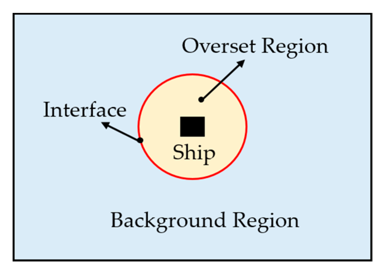
2.1. Definition of the Overset Mesh
2.2. Interpolation Option
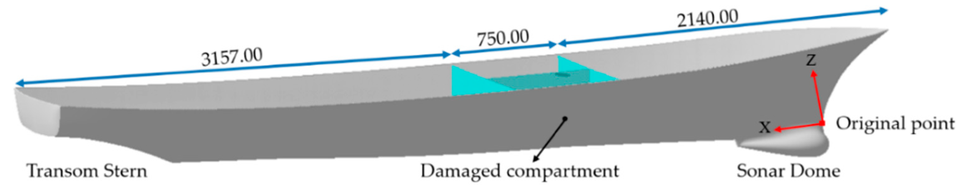
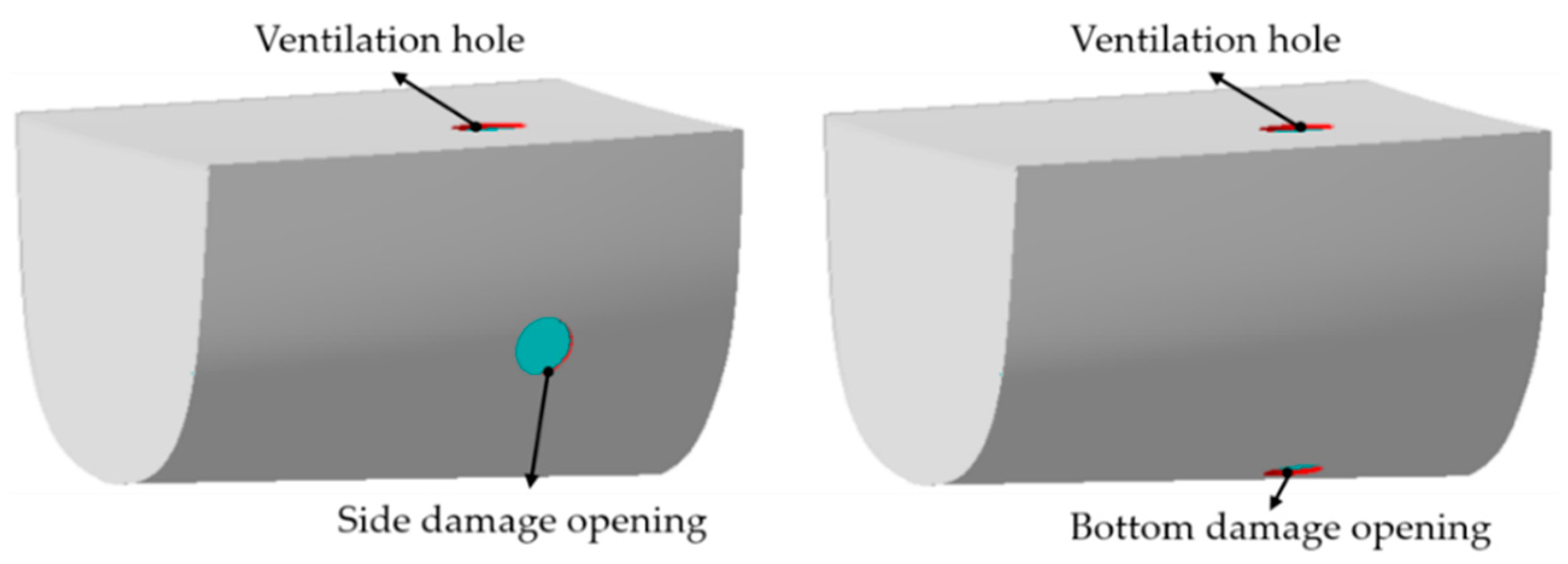
3. Model Description
4. Numerical Setup
4.1. Simulation Domain and Physical Models
4.2. Boundary Conditions and Solver Settings
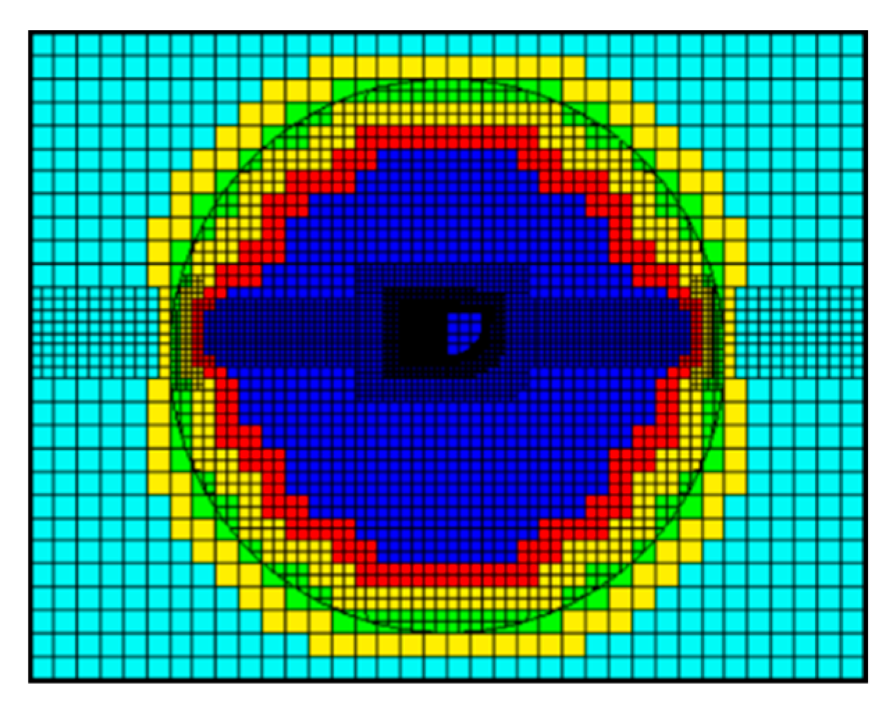
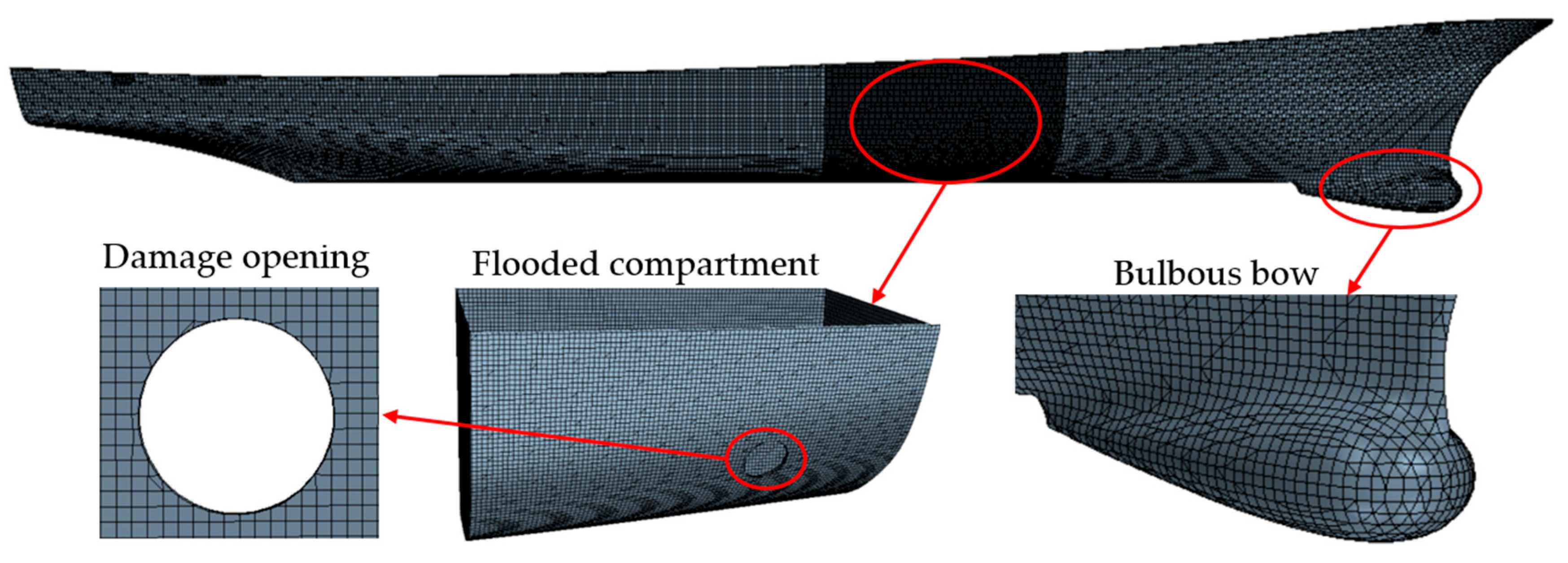
4.3. Mesh Type and Mesh Size
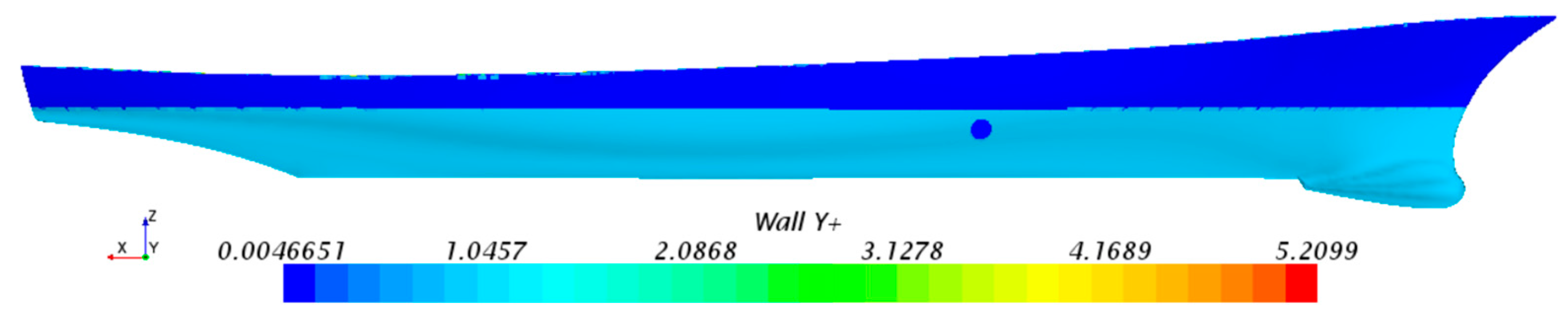
4.4. Near-Wall Treatment
5. Simulation Results and Discussion
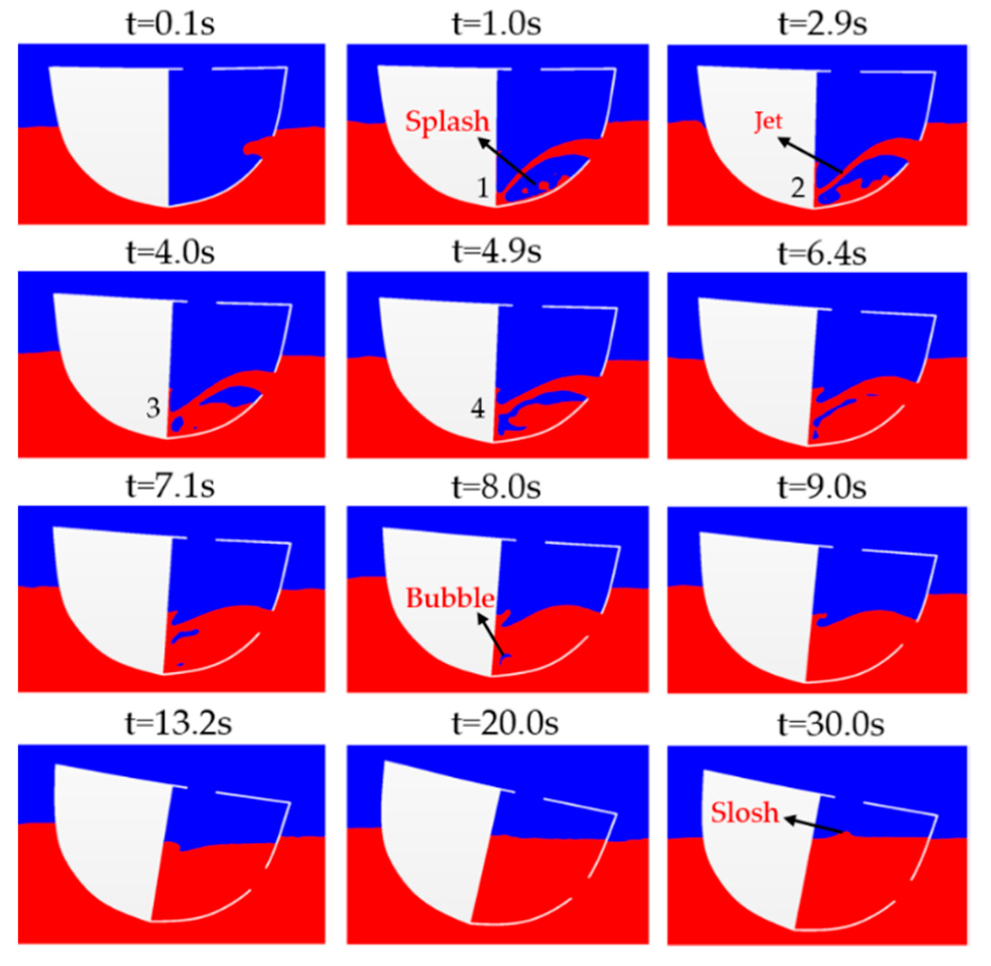
5.1. The Analysis of the Flooding Process in the Side Damage Scenario
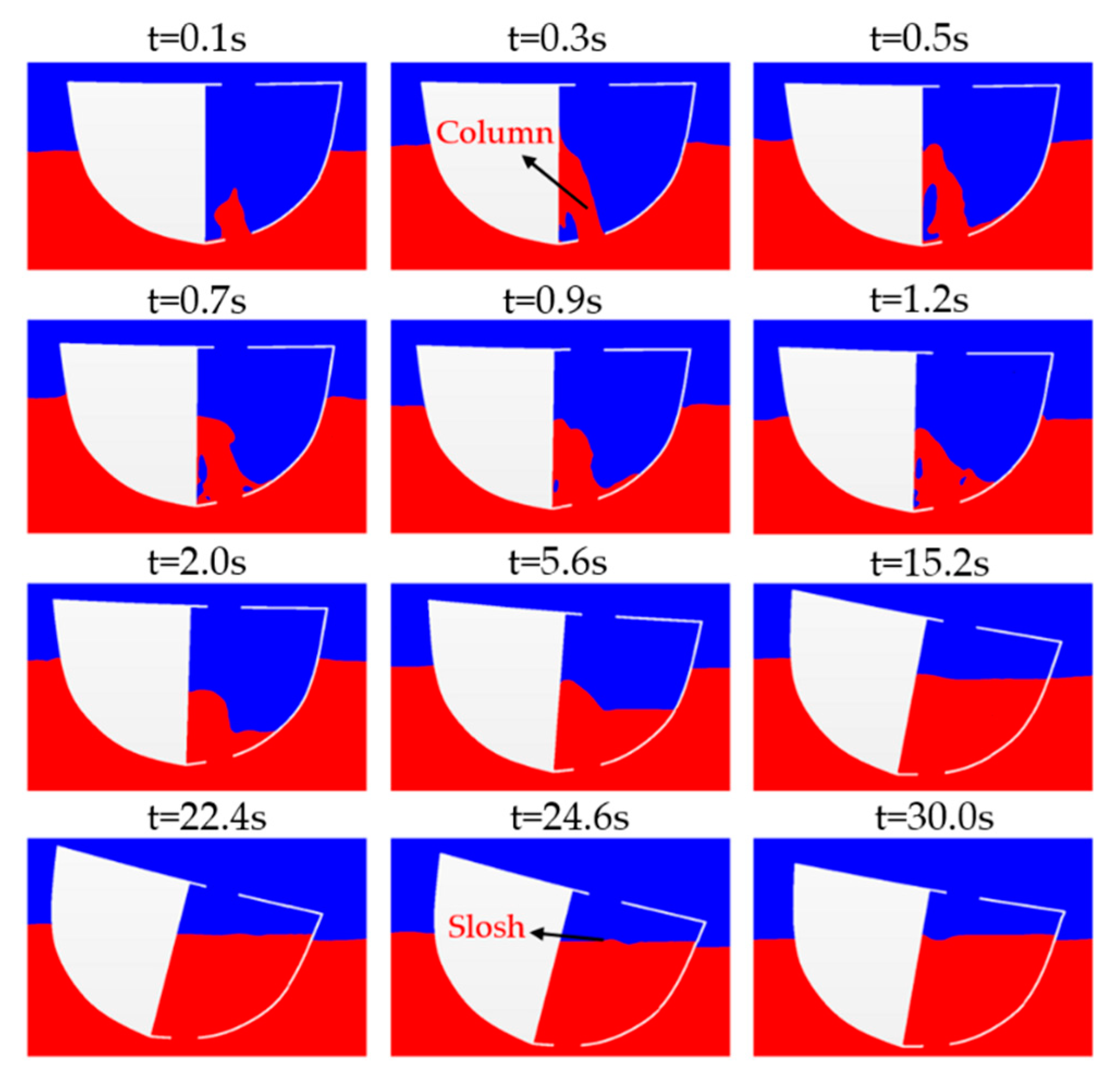
5.2. The Analysis of the Flooding Process in the Bottom Damage Scenario
5.3. The Analysis of the Coupled Motion Responses
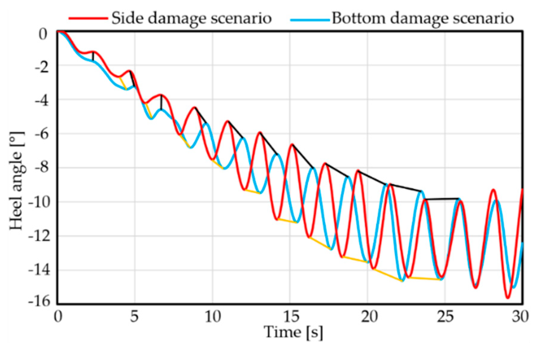
5.3.1. Description of the Roll Motion Response
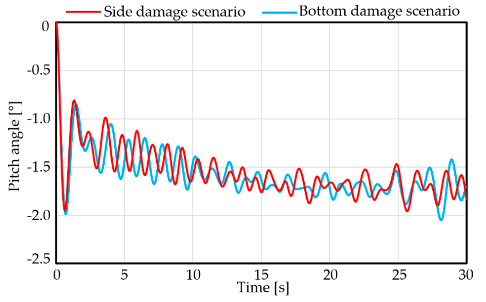
5.3.2. Description of the Pitch Motion Response
6. Conclusion and Future Researches
Author Contributions
Funding
Acknowledgments
Conflicts of Interest
References
- Manderbacka, T.; Themelis, N.; Bačkalov, I.; Boulougouris, E.; Eliopoulou, E.; Hashimoto, H.; Konovessis, D.; Leguen, J.F.; González, M.M.; Rodríguez, C.A.; et al. An overview of the current research on stability of ships and ocean vehicles: The STAB 2018 perspective. Ocean. Eng. 2019, 186, 106090. [Google Scholar] [CrossRef]
- Gao, Z.; Gao, Q.; Vassalos, D. Numerical simulation of flooding of a damaged ship. Ocean. Eng. 2011, 38, 1649–1662. [Google Scholar] [CrossRef]
- ITTC. The specialist committee on prediction of extreme ship motions and capsizing. In Proceedings of the 27th International Towing Tank Conference, Copenhagen, Denmark, 31 August–5 September 2014. [Google Scholar]
- ITTC. Stability in Waves Committee, Final Report and Recommendation. In Proceedings of the 28th International Towing Tank Conference, Wuxi, China, 17–22 September 2017. [Google Scholar]
- Acanfora, M.; De Luca, F. An experimental investigation into the influence of the damage openings on ship response. Appl. Ocean. Res. 2016, 58, 62–70. [Google Scholar] [CrossRef]
- Lim, T.; Seo, J.; Park, S.T.; Rhee, S.H. Free-running Model Tests of a Damaged Ship in Head and Following Seas. In Proceedings of the 12th International Conference on the Stability of Ship and Ocean Vehicles, Glasgow, UK, 14–19 June 2015. [Google Scholar]
- Siddiqui, M.A.; Greco, M.; Lugni, C.; Faltinsen, O.M. Experimental studies of a damaged ship section in forced heave motion. Appl. Ocean. Res. 2019, 88, 254–274. [Google Scholar] [CrossRef]
- Rodrigues, J.M.; Lavrov, A.; Hinostroza, M.A.; Soares, C.G. Experimental and numerical investigation of the partial flooding of a barge model. Ocean. Eng. 2018, 16, 586–603. [Google Scholar] [CrossRef]
- Korkut, E.; Altar, M.; Incecik, A. An experimental study of motion behavior with an intact and damaged Ro-Ro ship model. Ocean. Eng. 2004, 31, 483–512. [Google Scholar] [CrossRef]
- Acanfora, M.; de Luca, F. An experimental investigation on the dynamic response of a damaged ship with a realistic arrangement of the flooded compartment. Appl. Ocean. Res. 2017, 69, 191–204. [Google Scholar] [CrossRef]
- Domeh, V.D.K.; Sobey, A.J.; Hudson, D.A. A preliminary experimental investigation into the influence of compartment permeability on damaged ship response in waves. Appl. Ocean. Res. 2015, 52, 27–36. [Google Scholar] [CrossRef][Green Version]
- Risto, J.; Pekka, R.; Mateusz, W.; Hendrik, N.; Sander, V. A Study on Leakage and Collapse of Non-Watertight Ship Doors under Floodwater Pressure. Mar. Struct. 2017, 51, 188–201. [Google Scholar]
- Gao, Z.; Vassalos, D.; Gao, Q. Numerical simulation of water flooding into a damaged vessel’s compartment by the volume of fluid method. Ocean. Eng. 2010, 37, 1428–1442. [Google Scholar] [CrossRef][Green Version]
- Sadat-Hosseini, H.; Kim, D.H.; Carrica, P.M.; Rhee, S.H. URANS simulations for a flooded ship in calm and regular beam waves. Ocean. Eng. 2016, 120, 318–330. [Google Scholar] [CrossRef]
- Santos Tiago, A.; Guedes Soares, C. Numerical assessment of factors affecting the survivability of damaged ro-ro ships in waves. Ocean. Eng. 2009, 36, 797–809. [Google Scholar] [CrossRef]
- Ming, F.R.; Zhang, A.M.; Cheng, H.; Sun, P.N. Numerical simulation of a damaged ship cabin flooding in transversal waves with Smoothed Particle Hydrodynamics method. Ocean. Eng. 2018, 165, 336–352. [Google Scholar] [CrossRef]
- Manderbacka, T.; Mikkola, T.; Ruponen, P.; Matusiak, J. Transient response of a ship to an abrupt flooding accounting for the momentum flux. J. Fluids Struct. 2015, 57, 108–126. [Google Scholar] [CrossRef]
- Acanfora, M.; Begovic, E.; De Luca, F. A Fast Simulation Method for Damaged Ship Dynamics. J. Mar. Sci. Eng. 2019, 7, 111. [Google Scholar] [CrossRef]
- Stern, F.; Yang, J.M.; Wang, Z.Y.; Sadat-Hosseini, H.; Mousaviraad, M.; Bhushan, S.; Xing, T. Computational ship hydrodynamics: Nowadays and way forward. Int. Shipbuild. Prog. 2013, 60, 3–105. [Google Scholar]
- SIEMENS. STAR-CCM+ Overset Mesh. Available online: https://mdx2.plm.automation.siemens.com/sites/default/files/flier/pdf/Siemens-PLM-CD-adapco-STAR-CCM-overset-mesh-fs-59886-A2.pdf (accessed on 25 August 2019).
- STAR-CCM+ Users’ Guide Version 12.02; CD-Adapco, Computational Dynamics-Analysis & Design; Application Company Ltd.: Melville, NY, USA, 2012.
- De Luca, F.; Mancini, S.; Miranda, S.; Pensa, C. An extended verification and validation study of CFD simulations for planing hulls. J. Ship Res. 2016, 60, 101–118. [Google Scholar] [CrossRef]
- Lee, Y.; Chan, H.S.; Pu, Y.; Incecik, A.; Dow, R.S. Global Wave Loads on a Damaged Ship. Ships Offshore Struct. 2012, 7, 237–268. [Google Scholar] [CrossRef]
- Cao, X.Y.; Ming, F.R.; Zhang, A.M. Multi-phase SPH modelling of air effect on the dynamic flooding of a damaged cabin. Comput. Fluids 2018, 163, 7–19. [Google Scholar] [CrossRef]
- Ruponen, P.; Kurvinen, P.; Saisto, I.; Harras, J. Air compression in a flooded tank of a damaged ship. Ocean. Eng. 2013, 57, 64–71. [Google Scholar] [CrossRef]
- Zhang, X.L.; Lin, Z.; Li, P.; Dong, Y.; Liu, F. Time domain simulation of damage flooding considering air compression characteristic. Water 2019, 11, 796. [Google Scholar] [CrossRef]
- Gao, Z.; Wang, Y.; Su, Y.; Chen, L. Numerical study of damaged ship’s compartment sinking with air compression effect. Ocean. Eng. 2018, 147, 68–76. [Google Scholar] [CrossRef]
- IMO MSC. 362 (92). Revised Recommendations on a Standard Method for Evaluating Cross-Flooding Arrangements. Adopted on 14 June 2013. Available online: http://www.imo.org/en/KnowledgeCentre/IndexofIMOResolutions/Documents/MSC - Maritime Safety/362(92).pdf (accessed on 23 December 2019).
- Mancini, S.; Begovic, E.; Day, A.H.; Incecik, A. Verification and validation of numerical modelling of DTMB 5415 roll decay. Ocean. Eng. 2018, 162, 209–223. [Google Scholar] [CrossRef]
- Handschel, S.; Köllisch, N.; Soproni, J.P.; Abdel-Maksoud, M. A numerical method for estimation of ship roll damping for large amplitudes. In Proceedings of the 29th Symposium on Naval Hydrodynamics, Gothenburg, Sweden, 26–31 August 2012. [Google Scholar]
- ITTC. Practical Guidelines for Ship CFD Applications. In ITTC Procedures and Guidelines; 7.5-03-02-03; ITTC: Rio de Janerio, Brazil, 2011. [Google Scholar]
- Tezdogan, T.; Demirel, Y.K.; Kellet, P.; Khorasanchi, M.; Incecik, A. Full-scale unsteady RANS CFD simulations of ship behavior and performance in head seas due to slow steaming. Ocean. Eng. 2015, 97, 186–206. [Google Scholar] [CrossRef]
- Zhang, X.L.; Lin, Z.; Mancini, S.; Li, P.; Li, Z.; Liu, F. A Numerical Investigation on the Flooding Process of Multiple Compartments Based on the Volume of Fluid Method. J. Mar. Sci. Eng. 2019, 7, 211. [Google Scholar] [CrossRef]
- Menter, F.R. Eddy Viscosity Transport Equations and Their Relation to the k-ε Model. J. Fluids Eng. 1997, 119, 876–884. [Google Scholar] [CrossRef]
- Begovic, E.; Day, A.H.; Incecik, A.; Mancini, S. Roll damping assessment of intact and damaged ship by CFD and EFD methods. In Proceeding of the 12th International Conference on the Stability of Ships and Ocean Vehicles, Glasgow, UK, 14–19 June 2015. [Google Scholar]
- Patankar, S.V.; Spalding, D.B. A calculation procedure for heat, mass and momentum transfer in three-dimensional parabolic flows. Int. J. Heat Mass Transf. 1972, 15, 1787–1806. [Google Scholar] [CrossRef]
- Weiss, J.M.; Maruszewski, J.P.; Smith, W.A. Implicit solution of preconditioned Navier–Stokes equations using algebraic multigrid. AIAA J. 1999, 37, 29–36. [Google Scholar] [CrossRef]
- Salim, S.M.; Cheah, S.C. Wall y+ Strategy for Dealing with Wall-bounded Turbulent Flows. In Proceedings of the International MultiConference of Engineers and Computer Scientists, Hong Kong, China, 18–20 March 2009. [Google Scholar]
- Rodi, W. Experience with Two-Layer Models Combining the k-ε Model with a One-equation Model near the Wall. AIAA Pap. 1991, 91-0216. [Google Scholar] [CrossRef]
- Ruponen, R.; Queutey, P.; Kraskowski, M.; Jalonen, R.; Guilmineau, E. On the calculation of cross-flooding time. Ocean. Eng. 2012, 40, 27–39. [Google Scholar] [CrossRef]


| Parameters | Particulars | Real Ship | Scale Model (1/25) |
|---|---|---|---|
| Length Overall | (m) | 151.1800 | 6.0470 |
| Length between perpendiculars | (m) | 142.0400 | 5.6856 |
| Breadth at Waterline | (m) | 20.0300 | 0.8012 |
| Depth to public spaces deck | D (m) | 12.7400 | 0.5096 |
| Design draft | T (m) | 6.3100 | 0.2524 |
| Volume | V () | 8811.94 | 0.5640 |
| Maximum section area | () | 96.7923 | 0.1549 |
| Block coefficient | 0.4909 | 0.4909 | |
| Prismatic coefficient | 0.6409 | 0.6409 | |
| Midship section coefficient | 0.7658 | 0.7658 | |
| Height of metacenter above keel | KM (m) | 9.4700 | 0.3788 |
| Height of Centre of Gravity above keel | KG (m) | 6.2830 | 0.2513 |
| Metacentric height | GM (m) | 3.1870 | 0.1272 |
| Parameters | Unit | Side/Bottom Damage Scenario | |
|---|---|---|---|
| Total Weight | kg | 665.64 | |
| Ventilation hole | mm | Radius | 50 |
| Damage opening | mm | Radius | 40 |
| Center of mass x | mm | 2750.388 | |
| Center of mass y | mm | −0.0260 | |
| Center of mass z | mm | 293.040 | |
| Inertia moment | 60.3880 | ||
| Inertia moment | 1816.394 | ||
| Inertia moment | 1832.41 | ||
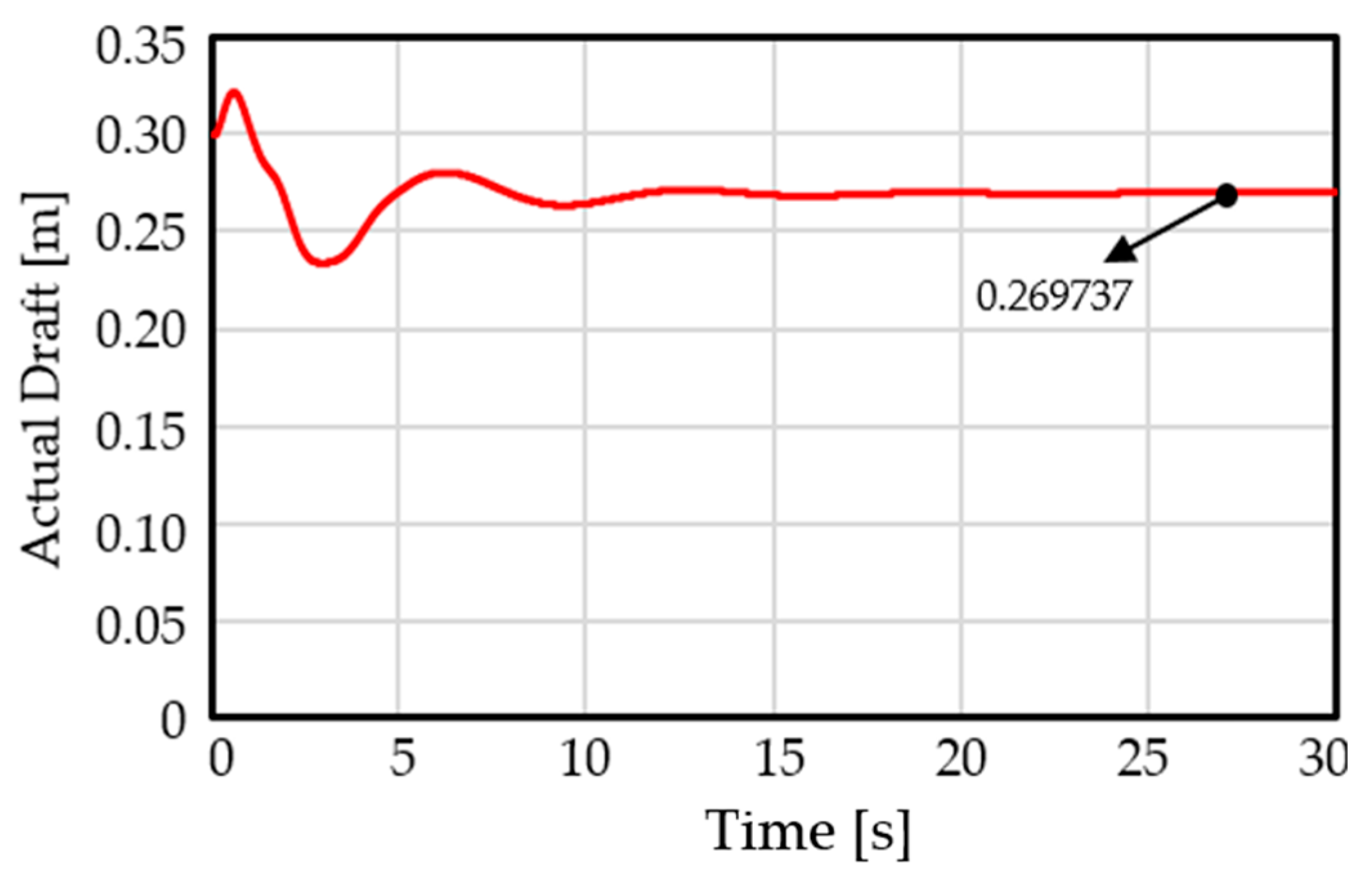
| Actual draft | m | 0.269737 | |
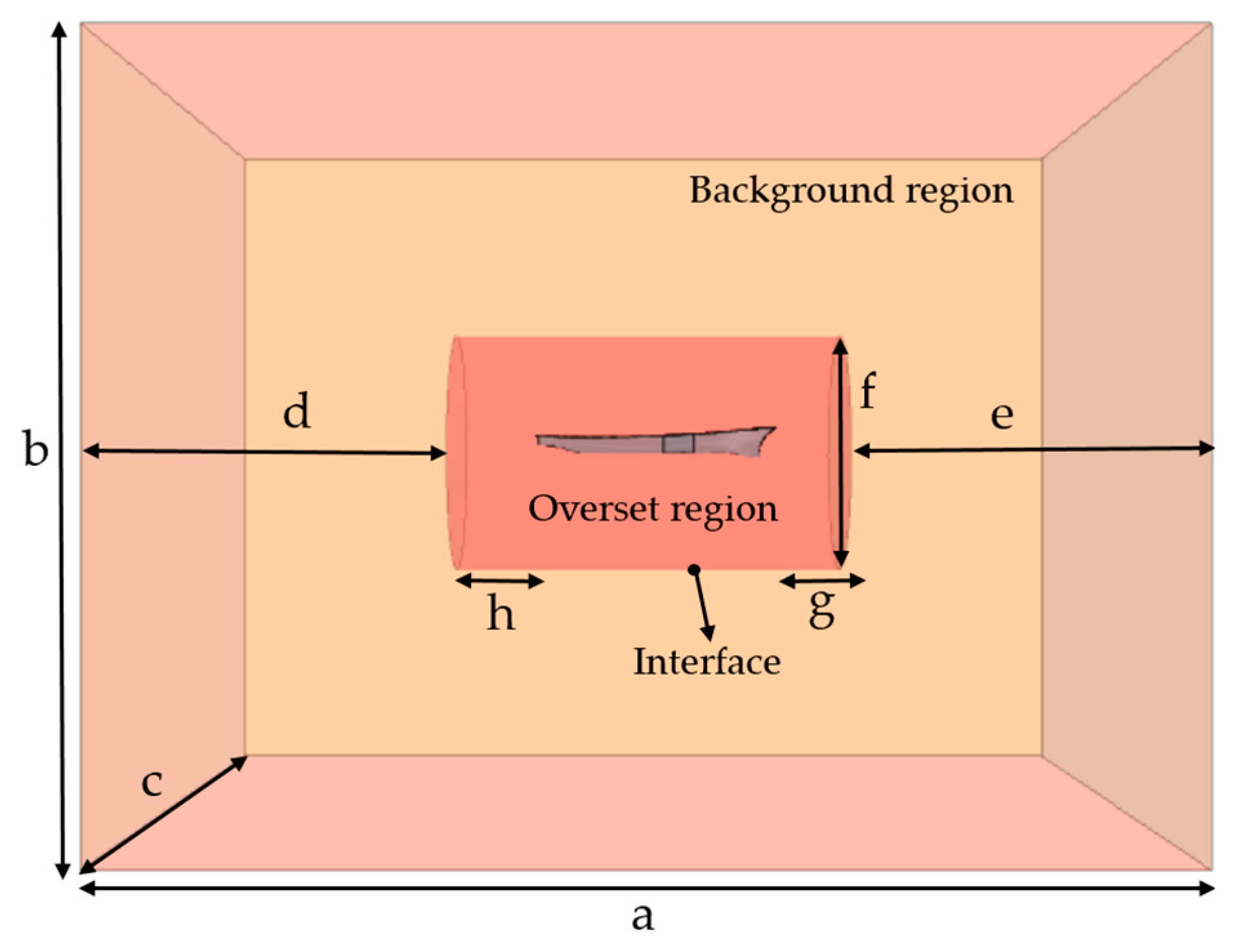
| Description | Symbol | Dimension | Mancini et al. [29] | Handschel et al. [30] |
|---|---|---|---|---|
| Domain length | a | 4.0 | 4.7 | 3.6 |
| Domain height | b | 3.0 | 2.7 | 1.8 |
| Domain breath | c | 3.0 | 3.4 | 1.2 |
| Inlet/outlet to cylinder | d,e | 1.2 | 1.7 | 1.2 |
| Cylinder to ship | h,g | 0.3 | 0.3 | 0.1 |
| Cylinder diameter | f | 3.75 | 4.7 | 2.0 |
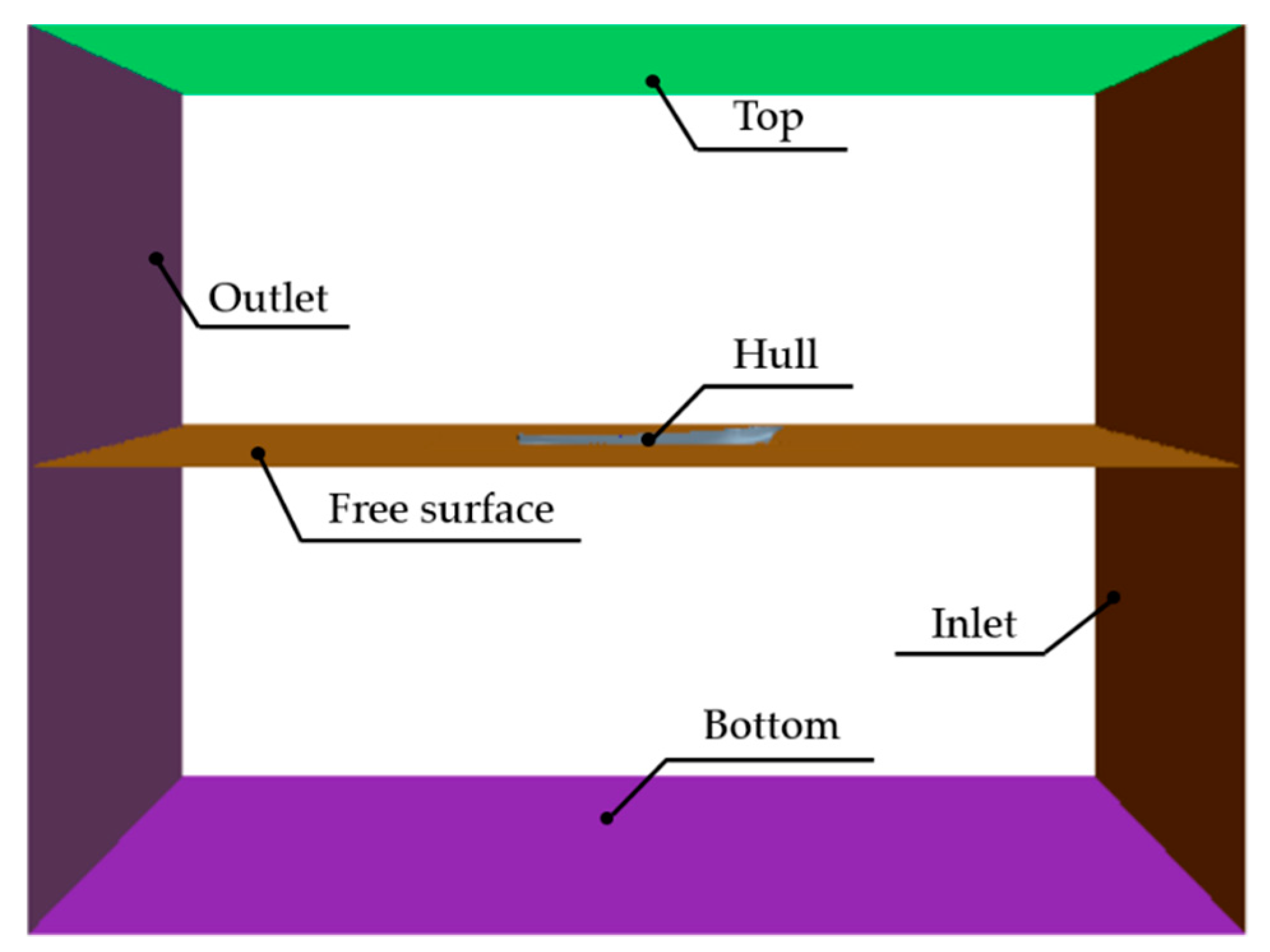
| Boundary Name | Boundary Type (This Paper) | Boundary Type Begovic et al. [35] | Boundary Type Zhang et al. [33] |
|---|---|---|---|
| Inlet | Velocity inlet | Velocity inlet | Velocity inlet |
| Outlet | Velocity inlet | Velocity inlet | Pressure outlet |
| Top/Bottom | Velocity inlet | Velocity inlet | Velocity inlet |
| Sides | Pressure outlet | Pressure outlet | Symmetry plane |
| Hull | Wall | Wall | Wall |
| Time step (s) | 0.002 | 0.001 | 0.004 |
| Maximum inner iterations | 10 | 12 | 10 |
| Convection Term | Second-order | Second-order | Second-order |
| Temporal Discretization | Second-order | Second-order | Second-order |
| Part | Affiliated Region | Wrapper Size | Remesh Size | Trim Size |
|---|---|---|---|---|
| Bulbous bow | Overset region | 0.050 m | 0.015 m | 0.110 m |
| Damage opening | Overset region | 0.050 m | 0.010 m | 0.110 m |
| Ventilation hole | Overset region | 0.050 m | 0.010 m | 0.110 m |
| Ship | Overset region | 0.100 m | 0.015 m | 0.110 m |
| Flooded compartment | Overset region | 0.060 m | 0.015 m | 0.010 m |
| Overlapping region | Overset region | 0.100 m | 0.250 m | 0.110 m |
| Overlapping region | Background region | None | 0.250 m | 0.250 m |
| Free surface | Overset region | 0.100 m | 0.250 m | 0.060 m |
| Free surface | Background region | None | 0.250 m | 0.120 m |
© 2019 by the authors. Licensee MDPI, Basel, Switzerland. This article is an open access article distributed under the terms and conditions of the Creative Commons Attribution (CC BY) license (http://creativecommons.org/licenses/by/4.0/).
Share and Cite
Zhang, X.; Lin, Z.; Mancini, S.; Li, P.; Liu, D.; Liu, F.; Pang, Z. Numerical Investigation into the Effect of Damage Openings on Ship Hydrodynamics by the Overset Mesh Technique. J. Mar. Sci. Eng. 2020, 8, 11. https://doi.org/10.3390/jmse8010011
Zhang X, Lin Z, Mancini S, Li P, Liu D, Liu F, Pang Z. Numerical Investigation into the Effect of Damage Openings on Ship Hydrodynamics by the Overset Mesh Technique. Journal of Marine Science and Engineering. 2020; 8(1):11. https://doi.org/10.3390/jmse8010011
Chicago/Turabian StyleZhang, Xinlong, Zhuang Lin, Simone Mancini, Ping Li, Dengke Liu, Fei Liu, and Zhanwei Pang. 2020. "Numerical Investigation into the Effect of Damage Openings on Ship Hydrodynamics by the Overset Mesh Technique" Journal of Marine Science and Engineering 8, no. 1: 11. https://doi.org/10.3390/jmse8010011
APA StyleZhang, X., Lin, Z., Mancini, S., Li, P., Liu, D., Liu, F., & Pang, Z. (2020). Numerical Investigation into the Effect of Damage Openings on Ship Hydrodynamics by the Overset Mesh Technique. Journal of Marine Science and Engineering, 8(1), 11. https://doi.org/10.3390/jmse8010011