The Flow Noise Calculation for an Axisymmetric Body in a Complex Underwater Environment

Abstract

The flow noise of a sonar platform is one of the main background interferences for sonar applications. This paper focuses on the flow noise of an axisymmetric body in a complex oceanic environment. Under the condition of a constant stream velocity which comes from the axial direction, an analytical method for computing the flow noise power spectrum in the transition region of the axisymmetric body is given in detail. The flow noise power spectrum computed by the analytical method is in agreement with the numerical simulation result. Then the flow noise physical features of the axisymmetric body in different incoming stream directions and velocity states caused by the complex oceanic environment are computed and analyzed by the numerical method. The results show that as the incoming stream direction changes, the transition region will migrate and the flow noise radiation direction of the axisymmetric body will also rotate at an angle which equals the stream direction variation. The flow noise energy generated by other directional incoming streams is slightly larger than that generated by the stream coming from an axial direction. When the incoming stream velocity is time-varying, the vorticity change on the axisymmetric body surface is obviously stronger than that under a constant stream, and the generated flow noise energy is also significantly larger. In addition, it indicates that there is a significant correlation between the intensity of flow noise energy and the magnitude of flow velocity.

1. Introduction

The noise sources of the underwater vehicle and other axisymmetric bodies include hydrodynamic, mechanical, and propeller noises. When the sailing speed of an axisymmetric body increases to a certain value, hydrodynamic noise will become the main noise source which is dominated by flow noise [1]. The noise comes from the turbulent pulsating pressure generated at the wall of the body surface due to the interaction between the shell and the fluid, which is usually referred to as flow noise [2,3]. The flow noise is one of the main interference backgrounds that limits the performance of sonar mounted on an underwater platform; it reduces the signal-to-noise ratio of sonar and shortens the sonar detection range. In addition, it will radiate as a target sound source to a distant place [4,5]. Due to the actual oceanic environment being very complex, such as existing surface sea waves, ocean currents, and other disturbance factors, disturbance factors will cause an angle of attack between the axis of the axisymmetric body and its motion direction, and they could also lead to the motion speed of the axisymmetric body to be time-varying [6,7]. Therefore, it is of great significance to study the flow noise of an axisymmetric body in a complex underwater environment.

At present, there are two approaches used to research the flow noise of the axisymmetric body: experimental measurement [8,9,10,11,12] and numerical calculation [13,14,15]. The results of the experimental measurement are true and reliable, but they could be affected by interference noise and be limited by experimental conditions [8]. Theoretical and experimental studies [9,10,11,12] have shown that the flow noise around the head of the axisymmetric body comes mainly from the radiated noise of the boundary layer transition region. The levels of pressure fluctuations in the transition region have been found to be significantly higher than those in the fully developed region of turbulent flow. The experimental study by Lauchle [9] showed that the transition from laminar to turbulent flow on the body appears to be an important source of flow noise.

Numerical studies of the flow noise started with Lighthill’s acoustic analogy theory [16,17]. The Lighthill equation was derived from the Navier–Stokes (NS) equation of fluid mechanics. In recent year, the Ffowcs Williams–Hawkings (FW-H) equation [18], which was developed from the Lighthill equation, has been used for the prediction of the flow noise. Farassat et al. [19,20,21] presented the solution for the FW-H equation. An analytical calculation and numerical analysis of the physical features of the flow noise for an axisymmetric body were presented by Li [13]. However, the methods for calculating the surface pressure coefficient of the axisymmetric body and the displacement thickness difference of the transition region used in the analytical formula were not given. In addition, the incoming stream velocity magnitude studied in literature is constant and comes from the axial direction. In [15], Yao et al. presented a numerical flow noise calculation method based on boundary elements. The difference between the FW-H method and the boundary element method in calculating acoustic noise was compared and analyzed. But the two methods are both numerical which are based on the finite element, and the flow noise was calculated under the conditions that when the incoming stream direction is horizontal, the incoming stream velocity is constant. Gross et al. [22,23] studied the fluid separation of three-dimensional hemisphere-cylinders at different angles of attack from the flow field analysis perspective, but not involved the analysis of the sound field. Shi et al. [24] combined the large eddy simulation method with the Lighthill acoustic analogy theory to simulate the flow noise for an unmanned underwater vehicle with full appendages under different angles of attack. The numerical results showed that the angle of attack has little effect on the flow noise level of the vehicle while the angle ranges from 0° to 4°. The numerical studies about the flow noise of an underwater axisymmetric body in [25,26,27] were also under the condition of a constant stream velocity which comes from the axial direction.

To date, the studies about flow noise are mainly by numerical calculation, and the analytical method for computing the flow noise of the axisymmetric body is scarce. In addition, the influences of the variations of the incoming stream velocity and direction on the numerical calculation of the flow noise are not considered; these assumed calculation conditions are inconsistent with the real underwater environment.

The objective of this paper is to analyze the flow noise of the axisymmetric body in a complex oceanic environment, which means the incoming stream velocity is time-varying, and the incoming stream comes from different directions. To achieve the objective, an analytical method based on Liepmann’s theory for calculating the flow noise of the transition region of the axisymmetric body is given. The methods for solving the surface pressure coefficient, the transition region length, and the displacement thickness difference in the analytical method are proposed and given in detail. Using the numerical calculation method, the flow noise features of the axisymmetric body in different incoming stream directions and different incoming stream velocity states caused by the complex oceanic environment are computed and analyzed. The results show that the flow noise energy is higher when the stream comes from other directions or the stream velocity is time-vary compared with that under the condition in the aforementioned studies. Accordingly, the radiation direction of the flow noise will rotate with the change of incoming stream direction. The paper is arranged as follows. A detailed analytical method for calculating the flow noise in the transition region of an axisymmetric body is presented in Section 2. The methods for solving the surface pressure coefficient of the axisymmetric body, the length of the transition region, and the displacement thickness difference of the transition region are presented. The theory about the numerical calculation method of the flow noise is given in Section 3. Section 4 presents the analytical and numerical results. The conclusions are presented in Section 5.

2. Analytical Calculation Method

A boundary layer will form when the stream passes the axisymmetric body. There are three flow states in the boundary layer of the axisymmetric body, as shown in Figure 1. When the axisymmetric body moves in water, the boundary layer near the stagnation point remains laminar flow, and subsequently, it changes from a transition status to turbulence status. Related research carried out by Lauche [10,11] showed that the noise measured in the laminar region (including the stagnation point) corresponds closely to that measured in the transition region. It indicates that the noise signal received by the acoustic pressure transducer on the head of the axisymmetric body comes mainly from the transition region.

Based on Liepmann’s theory and without considering the acoustic diffraction loss of sound waves at the head of the axisymmetric body, the sound power spectrum that is received at the stagnation point of the axisymmetric body can be written as [28]

$$\Phi \left(r,f\right)=\frac{{\rho }^2{V}_{\infty }{u}_c\Delta {\delta }^{*}{}^{2}L{(k_c\Delta x)}^2}{8{\pi }^2{r}^2[1+{(k_c\Delta x)}^2]{\left(\frac{t_i{u}_c}{\Delta x}\right)}^2}F(k_c\Delta x),$$

(1)

where

$$F(k_c\Delta x)={(k_c\Delta x)}^2{\displaystyle {\int }_0^1{\displaystyle {\int }_{-z}^{1-z}\frac{z{N}^{*}\gamma \cos (k_c\Delta xy)e^{-{\alpha }^{*}\Delta x\left|y\right|}}{4N^{*2}{\left(\frac{V_{\infty }}{u_c}\right)}^2+{(k_c\Delta x)}^2}}}dydz,$$

(2)

and

$$N^{*}=N·\Delta x/u_c,$$

(3)

$${\alpha }^{*}=\frac{1+83.35z^8}{\Delta x};$$

(4)

where L is the circumference of the axisymmetric body in the position where the transition region is located; k_c is the wavenumber, and k_c = ω/u_c; ω is the radian frequency; V_∞ is the free stream flow velocity; u_c = 0.8V_∞ is the turbulent spot convection velocity; ρ is the fluid density; Δδ* denotes the displacement thickness of the transition; Δx is the length of the transition region; r is the axial length from the transition region to the stagnation point; $\gamma (z)$ is the intermittency factor; and N(z) is the burst frequency. The experiment [29] showed that the dimensionless rise time (t_iu_c/Δx) is between 0.05 and 1.36. It is generally taken as 0.5.

According to Josserand’s experimental data [30],

$$N(z)=2.38\frac{V_{\infty }}{\Delta x}\sqrt{(1-\gamma (z))\mathrm{In}\frac{1}{1-\gamma (z)}},$$

(5)

$$\gamma (z)=1-{\mathrm{e}}^{-(1+3.4z)z^2}.$$

(6)

From Equation (1), it can be seen that it is necessary to estimate the length Δx and the displacement thickness difference Δδ* of the transition region before calculating its radiated noise power spectrum. In addition, the pressure coefficient of the surface of the axisymmetric body must be obtained first before calculating the length of the transition region and the difference of the displacement thickness. The calculation methods of the surface pressure coefficient, the length of the transition region, and the displacement thickness of the axisymmetric body, are given below.

2.1. Panel Method for Computing the Pressure Distribution

The panel method is adopted to compute the pressure coefficient distributed on the surface of the axisymmetric body [31,32]. The panel method with a basic source-sink distribution is used in the calculation of the potential flow. It divides the surface of the body into N small panels in some way. The source-sink density is distributed on the small panel. The source density is solved according to the boundary conditions, and then the velocity and pressure distributions of the flow field can be obtained. The basic equation of the method of source-sink distribution is given as

$$2\pi \sigma (P)-{\displaystyle {\iint }_s\frac{\partial }{\partial n}}(\frac{1}{r_{PQ}})\sigma (Q)\mathrm{d}S=-{\mathit{V}}_{\infty }·\mathit{n}(P),$$

(7)

where P is the point on the boundary surface where the potential and velocity are evaluated; Q is the point where source is located, especially a point on the boundary surface; S denotes the boundary surface on which the flow is calculated; n is the unit normal vector; V_∞ is the incoming stream velocity; σ is the surface source density; and r_PQ is the distance between two points in three-dimensional space, especially between the source and where the potential velocity is evaluated.

To solve Equation (7), a set of linear algebraic equations can be used to approximate the integral equation. Assuming that the number of surface elements which was used to approximate the surface of the body is N, and the source density, which is uniformly distributed on each element is σ_j. j or i, which represents the serial number of the element, and is also used to identify the control points and the physical quantities therein. By applying integral Equation (7) to the control point i can obtain the following equation:

$${\displaystyle \sum _{j=1}^N{\sigma }_j}\left[-{\displaystyle {\iint }_{s_j}\frac{\partial }{\partial n_i}}(\frac{1}{r_{ij}})dS+2\pi {\delta }_{ij}\right]=-{\mathit{V}}_{\infty i}·{\mathit{n}}_i,$$

(8)

where n_i is the unit normal vector to the ith element; δ_ij is the Dirac function, and ${\delta }_{ij}=\{\begin{array}{ll}1,& i=j\\ 0,& i\ne j\end{array}$.

The physical meaning expressed in the left parenthesis of Equation (8) is that when the source density distributed on the jth surface element is the unit value, the contributions of the source density to the normal velocity of the control point on the ith surface element, which is called the normal velocity, influence the coefficient.

When i changes from 1 to N, Equation (8) becomes a system of equations with N unknown σ_j and N linear algebraic equations, and the normal velocity influence coefficient also becomes an element in the normal velocity influence coefficient matrix. If it is represented by A_ij, then Equation (8) can be written as

$${\displaystyle \sum _{j=1}^N{A}_{ij}}{\sigma }_j=-{\mathit{V}}_{\infty i}·{\mathit{n}}_i(i=1,2,\cdots N).$$

(9)

Equation (9) is used to replace the original integral equation. Solving the equation can obtain the source density σ_j.

For a general three-dimensional flow, the velocity influence factor v_ij can be expressed in three components, which is

$${\mathit{v}}_{ij}=v_{xij}\mathit{i}+v_{yij}\mathit{j}+v_{zij}\mathit{k},$$

(10)

where i, j, and k are the unit vectors along the axes of the reference coordinate system; and v_xij, v_yij, and v_zij are simply the components of v_ij.

The normal velocity influence coefficient A_ij is the projection of v_ij in the n_i direction, which is

$$A_{ij}={\mathit{v}}_{ij}·{\mathit{n}}_i.$$

(11)

The total velocity at the control point is expressed as the sum of disturbance velocity and incoming flow velocity as follows:

$${\mathit{V}}_i={\mathit{v}}_i+{\mathit{V}}_{\infty i}={\displaystyle \sum _{j=1}^N{\mathit{v}}_{ij}}{\sigma }_j+{\mathit{V}}_{\infty i}.$$

(12)

In summary, the surface pressure C_pi distribution can be obtained as follows:

$$C_{pi}=1-{(\frac{V_i}{V_{\infty i}})}^2.$$

(13)

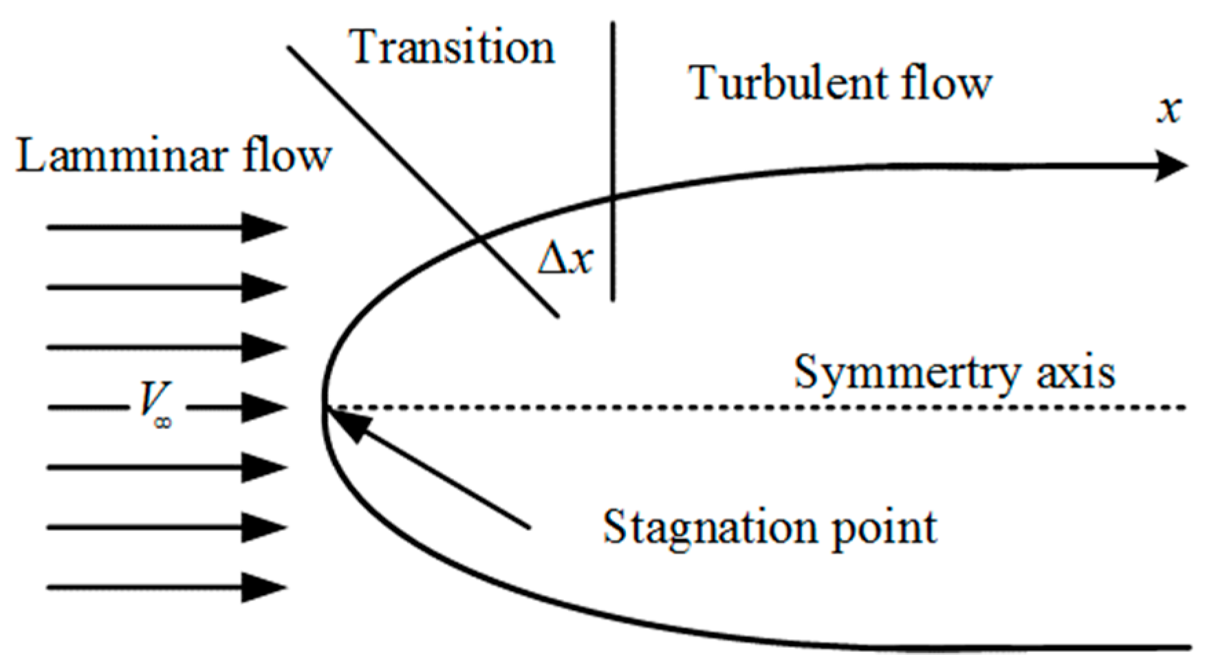
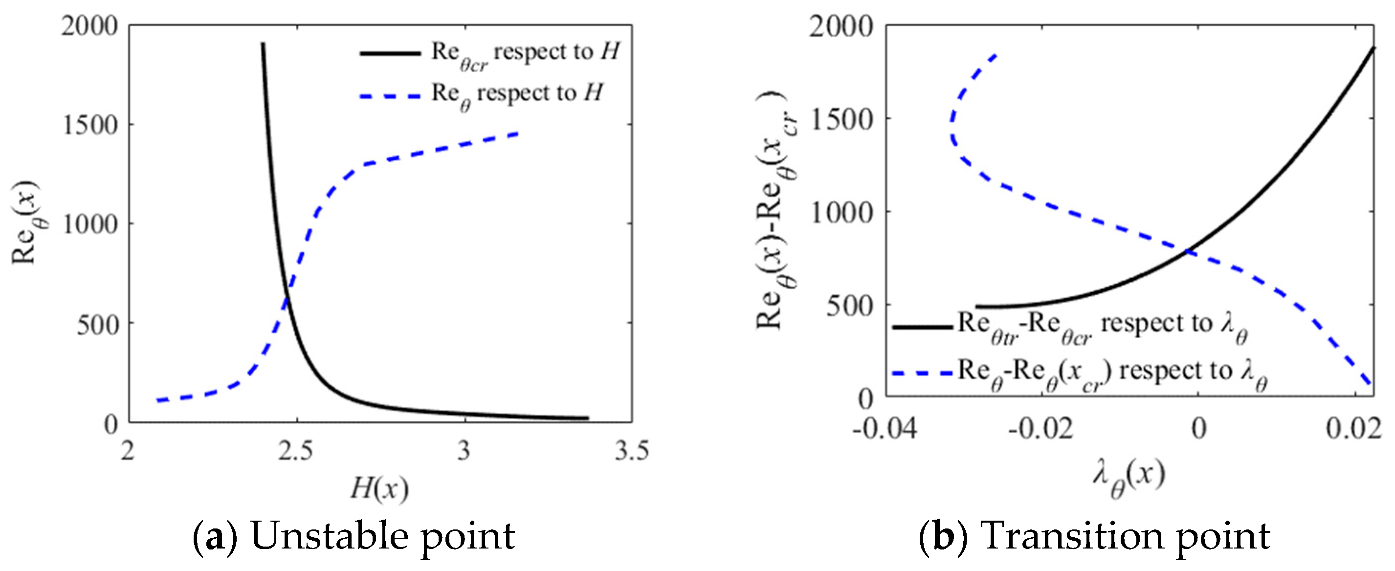
2.2. Calculation of the Transition Region Length

The Granville method [13,33] is used to compute the length of the transition region of the axisymmetric body. The single parameter momentum integral method improved by Holstein and Bohlen [34] is used to solve the laminar boundary layer.

The momentum loss thickness θ is given by

$${\theta }^2=\frac{0.45\upsilon }{r_0^2{V}_{\infty }^6}{\displaystyle {\int }_0^x{r}_0^2}{V}_{\infty }^{5}dx,$$

(14)

where ʋ is the kinematic viscosity coefficient; r₀ is the distance from the surface to the axis of the axisymmetric body, and V_∞ is the incoming stream velocity.

The dimensionless parameter λ proposed by Holstein and Bohlen is

$$\lambda =\frac{{\theta }^2}{\upsilon }\frac{d{V}_{\infty }}{dx}=\frac{{\theta }^2{V^{\prime }}_{\infty }}{\upsilon },$$

(15)

where ${V^{\prime }}_{\infty }=\frac{d{V}_{\infty }}{dx}$.

The shape factor H(λ) corresponding to the dimensionless parameter λ can be obtained according to the shape factor correlation function value given by Thwaites.

The momentum thickness Reynolds number ${\mathrm{Re}}_{\theta }$ is

$${\mathrm{Re}}_{\theta }=\frac{V_{\infty }\theta }{\upsilon }.$$

(16)

The displacement thickness δ* is computed from

$$\frac{{\delta }^{\ast }}{\theta }=H(\lambda ).$$

(17)

The momentum thickness Reynolds number Re_θcr at the unstable point is a function of the shape factor H [33]; which is given by

$${\mathrm{Re}}_{\theta cr}=\exp ({\displaystyle \sum _{n=0}^7{C}_n{H}^n}),$$

(18)

where C₀ = 493.906, C₁ = 407.017, C₂ = 53.9041, C₃ = 24.1642, C₄ = −0.104478, C₅ = −2.81454, C₆ = 0.355919, and C₇ = 0.012027.

The x coordinate corresponding to the intersection point between the function curve and the curve about Re_θ(x) and H(x) is the unstable point x_cr.

The laminar flow calculation method is still used in the boundary layer at the downstream section of the x_cr point. For each boundary layer at the section, Re_θ needs to be calculated, where ΔRe_θ = Re_θ(x) - Re_θ(x_cr), and λ_θ(x) is given by

$${\lambda }_{\theta }=\frac{4}{45}-\frac{1}{5\upsilon }\left[\frac{{\left(r_0^2{V}_{\infty }{\theta }^2\right)}_{x_{tr}}-{\left(r_0^2{V}_{\infty }{\theta }^2\right)}_{x_{cr}}}{{\displaystyle {\int }_{x_{cr}}^{x_{tr}}{r}_0^2(x)dx}}\right].$$

(19)

The x coordinate of the intersection point between the curve of ΔRe_θ and the curve of Re_θtr-Re_θxr is the unstable point x_tr. The function curve of Re_θtr-Re_θxr with respect to λ_θ is given by [33]

$${\mathrm{Re}}_{\theta tr}-{\mathrm{Re}}_{\theta cr}={\displaystyle \sum _{n=0}^4{D}_n}{\lambda }_{\theta }^n,$$

(20)

where D₀ = 820.571, D₁ = 28,273.8, D₂ = 707,219, D₃ = 5,167,690, and D₄ = 22,302,300.

After obtaining the unstable point x_cr and the transition point x_tr of the axisymmetric body transition region, the length of the transition region can be obtained by

$$\Delta x=x_{tr}-x_{cr}.$$

(21)

2.3. Calculation of Displacement Thickness Difference

The calculation steps of the difference of the displacement thickness in the transition region are presented as follows. The Head’s method is used [33] to solve for the turbulent boundary layer of the axisymmetric body.

The calculation steps are as follows:

• The results of θ⁽ⁿ⁾ and H⁽ⁿ⁾ computed from the laminar boundary layer are taken as the initial values, where n denotes the unstable point;
• $H_1{}^{(n)}$ is computed from

  $$H_1(H)=\{\begin{array}{ll}0.8234{(H-1.1)}^{-1.287}+3.3& (H\le 1.6)\\ 1.5501{(H-0.6778)}^{-3.064}+3.3& (H\ge 1.6)\end{array};$$

  (22)
• F⁽ⁿ⁾ is computed from

  $$F(H_1)=0.0306{(H_1-3.0)}^{-0.6169},$$

  (23)

  where F means the growth rate of the volume flow in the boundary layer along the x direction, which is called the suction coefficient;
• $\frac{d({\theta }^{(n)}{H}_1{}^{(n)})}{dx}$ is computed from

  $$\frac{d(\theta H_1)}{dx}+\theta H_1(\frac{1}{V_{\infty }}\frac{d{V}_{\infty }}{dx}+\frac{1}{r_0}\frac{d{r}_0}{dx})=F;$$

  (24)
• ${\theta }^{(n+1)}{H}_1{}^{(n+1)}$ is computed from

  $${\theta }^{(n+1)}{H}_1{}^{(n+1)}={\theta }^{(n)}{H}_1{}^{(n)}+\frac{d({\theta }^{(n)}{H}_1{}^{(n)})}{dx}\Delta x;$$

  (25)
• $C_f^{(n)}$ is computed from

  $$C_f=0.246{(\frac{V_{\infty }\theta }{\upsilon })}^{-0.286}\times {10}^{-0.678H},$$

  (26)

  where C_f is the surface frictional stress coefficient;
• $\frac{d{\theta }^{(n)}}{dx}$ is computed from

  $$\frac{d\theta }{dx}+(2+H)\frac{\theta }{V_{\infty }}\frac{d{V}_{\infty }}{dx}+\frac{\theta }{r_0}\frac{d{r}_0}{dx}=\frac{1}{2}{C}_f;$$

  (27)
• θ⁽ⁿ⁺¹⁾ is computed from

  $${\theta }^{(n+1)}={\theta }^{(n)}+\frac{d{\theta }^{(n)}}{dx}\Delta x;$$

  (28)
• $H_1{}^{(n+1)}$ is computed from

  $$H_1{}^{(n+1)}=\frac{{\theta }^{(n+1)}{H}_1{}^{(n+1)}}{{\theta }^{(n+1)}};$$

  (29)
• H⁽ⁿ⁺¹⁾ is computed from

  $$H=\{\begin{array}{ll}{[\frac{1}{0.8234}(H_1-3.3)]}^{-\frac{1}{1.278}}+1.1& (H_1\ge 5.30)\\ {[\frac{1}{1.5501}(H_1-3.3)]}^{-\frac{1}{3.064}}+0.6678& (H_1<5.30)\end{array};$$

  (30)
• Then return to step 2, sequentially find all the θ and H in the transition region, and calculate the displacement thickness δ* according to Equation (17).

At last, the displacement thickness difference is computed from

$$\Delta {\delta }^{\ast }={\overline{\delta }}_T^{\ast }-{\overline{\delta }}_L^{\ast },$$

(31)

where ${\overline{\delta }}_L^{\ast }$ is the displacement thickness of the transition region of the boundary layer, which is calculated in the laminar boundary conditions; and ${\overline{\delta }}_T^{\ast }$ is the displacement thickness of the transition region of the boundary layer, which is calculated in the turbulent boundary conditions.

3. Numerical Calculation Method

3.1. Flow Field Control Equation

According to the law of mass conservation and momentum conservation, the Navier–Stokes (NS) equations of a three-dimensional incompressible viscous fluid can be written as [13]

$$\frac{\partial u_i}{\partial x_i}=0,$$

(32)

$$\frac{\partial u_i}{\partial t}+u_j\frac{\partial u_i}{\partial x_j}=f_i-\frac{1}{\rho }\frac{\partial p}{\partial x_i}+\frac{\partial }{\partial x_j}(\upsilon \frac{\partial u_i}{\partial x_j}-\overline{u_i^{\prime }{u}_j^{\prime }}),$$

(33)

where f_i is an external force; (x_i, x_j) denotes the particle coordinates and is the function on t; u_i and ${u^{\prime }}_j$ are the average velocity and the velocity fluctuation of the fluid, respectively; i, j = 1,2,3; ρ is the density of the fluid; p is the average pressure; and ʋ is the kinematical viscosity coefficient. $\overline{u_i^{\prime }{u}_j^{\prime }}$ is the Reynolds stress.

The RNG k-ε two-equation turbulent model used in this paper is given by

$$\frac{\partial }{\partial t}(\rho k)+\frac{\partial }{\partial x_j}(\rho k{u}_j)=\frac{\partial }{\partial x_j}\left[(\mu +\frac{{\mu }_t}{{\sigma }_k})\frac{\partial k}{\partial x_j}\right]+G_k-\rho \epsilon ,$$

(34)

$$\frac{\partial }{\partial t}(\rho \epsilon )+\frac{\partial }{\partial x_j}(\rho \epsilon u_j)=\frac{\partial }{\partial x_j}\left[(\mu +\frac{{\mu }_t}{{\sigma }_{\epsilon }})\frac{\partial \epsilon }{\partial x_j}\right]+C_{1\epsilon }\frac{\epsilon }{k}{G}_k-C_{2\epsilon }\rho \frac{{\epsilon }^2}{k},$$

(35)

where C_μ, σ_k, σ_ε, σ_1ε and σ_2ε are constants of the model.

3.2. Acoustic Field Control Equations

The Lighthill acoustic analogy theory is derived from the Navier–Stokes (NS) equation. In addition, the generalized Lighthill equation [16,17] in the acoustic analogy theory is used to calculate the noise field. Its density wave equation is in the form of

$$\frac{{\partial }^2{\rho }^{\prime }}{\partial t^2}-c_0^2{\nabla }^2{\rho }^{\prime }=\frac{{\partial }^2{T}_{ij}}{\partial x_i\partial x_j},$$

(36)

where ρ′ is the change in the density caused by fluid disturbance, ρ′ = ρ − ρ₀; ρ and ρ₀ denote the fluid densities with disturbance and without disturbance, respectively; T_ij is the Lighthill stress tensor $T_{ij}=\rho u_i{u}_j+P_{ij}-c_0^2{\delta }_{ij}{\rho }^{\prime }$, and $P_{ij}=p{\delta }_{ij}-\mu \left[(\partial u_i/\partial x_j)+(\partial u_j/\partial x_i)-(2/3)(\partial u_k/\partial u_k){\delta }_{ij}\right]$; c₀ is the sound speed in the fluid.

Ffowcs Williams and Hawkings [18] developed the Ffowcs Williams–Hawkings (FW-H) equation based on the basic equations of Lighthill using a generalized function theory.

$$\frac{1}{c_0^2}\frac{{\partial }^2{p}^{\prime }(x,t)}{\partial t^2}-{\nabla }^2{p}^{\prime }(x,t)=\frac{\partial }{\partial t}\left[{\rho }_0{U}_n\delta (f)\right]-\frac{\partial }{\partial x_i}\left[L_i\delta (f)\right]+\frac{{\partial }^2}{\partial x_i\partial x_j}[T_{ij}H(f)],$$

(37)

where $U_i=[1-(\rho /{\rho }_0)]{\nu }_i+(\rho u_i/{\rho }_0)$; $L_i=P_{ij}{\widehat{n}}_j+\rho u_i(u_n-v_n)$; p′ is the sound pressure in the far field condition, $p^{\prime }=p-p_0$; δ(f) is the Dirac delta function, f is the wall function; H(f) is Heaviside function; u is the fluid velocity; v is the body surface velocity; $c_0$ is the speed of sound in the far field; and n_j is the unit normal vector pointing from the periphery of the solid to the flow field. The three terms on the right of FW-H equation represent monopole, dipole, and quadruple noises, respectively [35].

The solution process of FW-H equation can be divided into two steps. First, the renormalization group (RNG) k-ε two equation turbulent models are adopted to obtain flow field data, so the intensity and distribution characteristics of sound sources near the wall can be extracted. Then, the sound field is solved by integral extrapolation of FW-H equation. Only when the velocity reaches the subsonic speed, it is necessary to consider the quadruple noise. In general, the noise sources of the underwater vehicle considered are only the monopole and dipole noises. Farassat et al. [20] proposed a solution for the FW-H equation, which retains only monopole and dipole noises. It can be expressed as a summation of two different terms yielding the total pressure disturbance at receiver location,

$$p^{\prime }(x,t)={p^{\prime }}_T(x,t)+{p^{\prime }}_L(x,t).$$

(38)

In the above (x,t) is the receiver location and time, ${p^{\prime }}_T$ and ${p^{\prime }}_L$ represent the monopole and dipole noises, respectively.

$$4\pi {p^{\prime }}_T(\overrightarrow{x},t)={\displaystyle {\int }_{f=0}{\left[\frac{{\rho }_0({\dot{U}}_n+U_{\dot{n}})}{r{(1-M_r)}^2}\right]}_{ret}}\mathrm{d}S+{\displaystyle {\int }_{f=0}{\left[\frac{{\rho }_0{U}_n(r{\dot{M}}_r+c_0(M_r-M^2))}{r^2{(1-M_r)}^3}\right]}_{ret}}\mathrm{d}S,$$

(39)

$$\begin{array}{l}4\pi {p^{\prime }}_L(\overrightarrow{x},t)=\frac{1}{c_0}{\displaystyle {\int }_{f=0}{\left[\frac{{\dot{L}}_r}{r{(1-M_r)}^2}\right]}_{ret}}\mathrm{d}S+{\displaystyle {\int }_{f=0}{\left[\frac{L_r-L_M}{r^2{(1-M_r)}^2}\right]}_{ret}}\mathrm{d}S\\ +\frac{1}{c_0}{\displaystyle {\int }_{f=0}{\left[\frac{L_r(r{\dot{M}}_r+c_0(M_r-M^2))}{r^2{(1-M_r)}^3}\right]}_{ret}}\mathrm{d}S\end{array}$$

(40)

In this paper, the solution of the flow field and FW-H equation are calculated by FLUENT software. In the sound field, the finite turbulent region with noise sources lies in an infinitely uniform, static acoustic medium, the reflection and scattering effects for sound propagation by the presence of boundaries and inhomogeneities are not considered. The numerical simulation results about pressure coefficient and flow noise power spectrum will be verified by analytical results.

4. Results and Analysis

The fore-body shape of the axisymmetric body selected in this paper is ellipsoidal, and the middle is cylindrical. The maximum length of the axisymmetric body is 2.6 m, and the maximum diameter is 0.3 m. The long and the short axes of the head ellipse are 0.3 m and 0.15 m, respectively.

4.1. Analytical Calculation Results

The process of the analytical method to calculate the flow noise is as follows. The calculation is under the condition of a constant stream velocity which comes from the axial direction.

1.

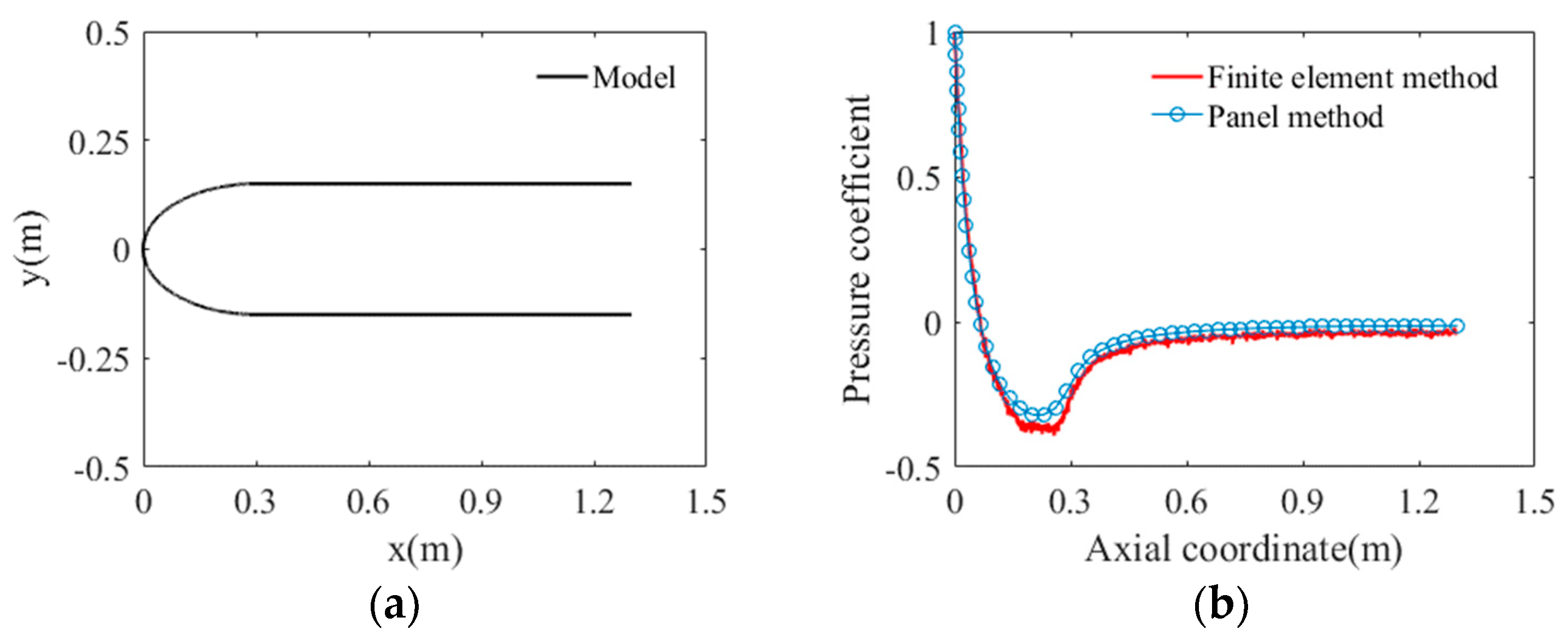
Calculation of the pressure coefficient

The pressure coefficient of the surface of the axisymmetric body calculated by the panel method is shown in Figure 2. The theoretical analysis calculation result can provide reference and comparison for verifying the accuracy of the method used for numerical simulation. Figure 2a shows a partial cross-sectional view of the axisymmetric body (XY section). The blue line in Figure 2b represents the pressure coefficient distributed on the section of the axisymmetric body in Figure 2a, which is calculated by the analytical method. Here, the incoming stream velocity V_∞ is 20 m/s.

2.

Calculation of the displacement thickness difference and the transition region length

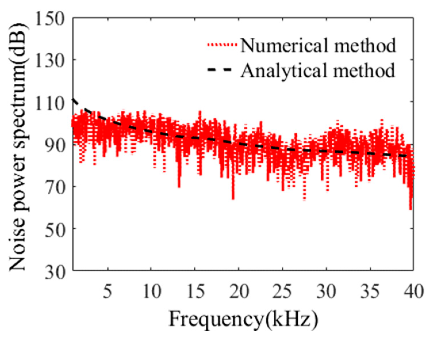
The dotted line in Figure 3a represents the curve of Re_θ. The solid line in Figure 3a represents the curve of Re_θcr given by Equation (18). The x-axis coordinate value of the intersection point in Figure 3a is the unstable point x_cr. The curve of ΔRe_θ with respect to λ_θ is represented by the dotted line in Figure 3b. The solid line in Figure 3b is given by Equation (20). The x coordinate value corresponding to the intersection point is the transition point x_tr.

By calculation, the length of the transition region of the model shown in Figure 2a is 0.0601 m. The laminar and turbulent flows exist simultaneously in the transition region. Here, the relevant parameters of the laminar flow corresponding to the unstable point are used as the initial conditions to solve the rest parameters of the turbulent flow in the transition region. The displacement thickness difference of the transition region of the model is 7.3479 × 10⁻⁵.

3.

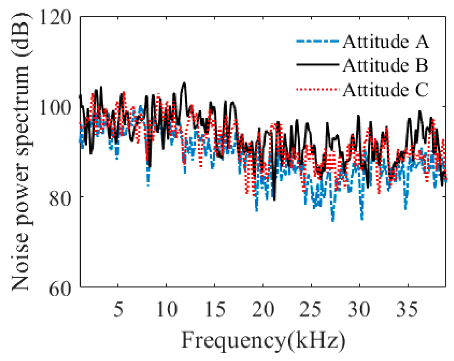
Calculation of the flow noise power spectrum

The black dotted line in Figure 4 represents the flow noise power spectrum at the stagnation point of the axisymmetric body, which is calculated by Equation (1) under the conditions when V_∞ = 20 m/s, ρ = 1000 kg/m³, L = 0.9420 m, and r = 0.3541 m. The reference sound pressure is 1 μPa.

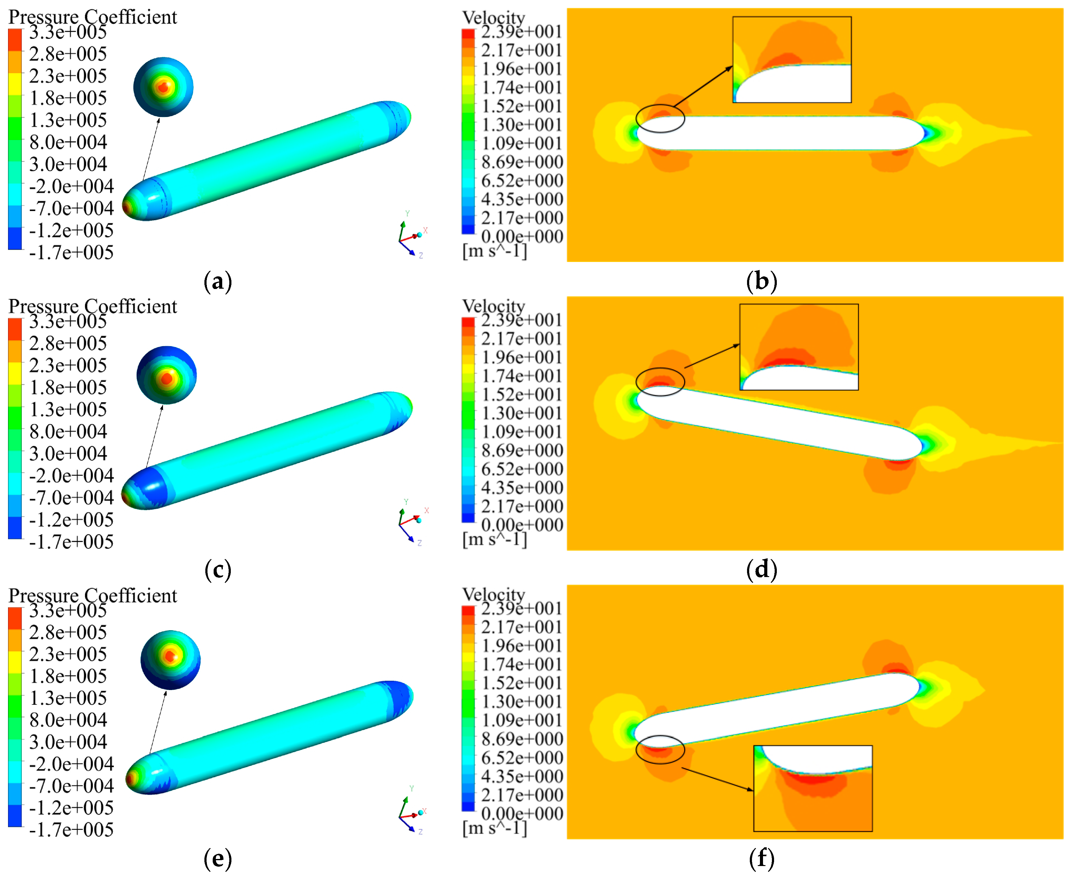
4.2. Numerical Calculation Results and Analysis

The flow noise power spectrum at the stagnation point of the axisymmetric body is calculated by computational fluid dynamics (CFD). The process of the numerical method is as follows. The calculation is under the condition of a constant stream velocity which comes from the axial direction.

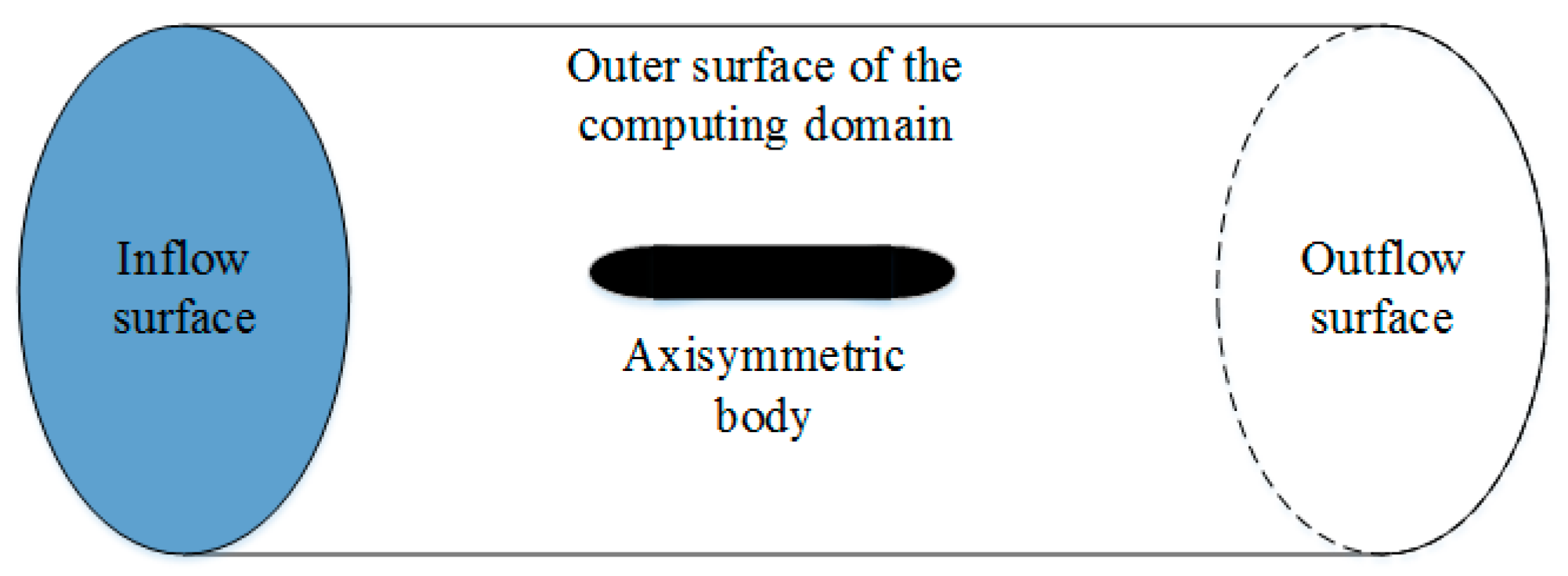
• Establishing a model. The model is established with reference to the actual size. The ratio is 1:1. The three-dimensional computing domain used in CFD is shown in Figure 5.
• Meshing the grid. The grid is chosen as body grid in the calculation of CFD. To fully capture the wall turbulent fluctuating pressure, the boundary layer grid is used in the meshing for the hydrophone solid wall surface.
• Setting flow field boundary conditions. The flow field calculation boundary conditions are shown in the

  Table 1. Boundary conditions of numerical calculation.

  Zone	Boundary Conditions
  Inflow surface Outflow surface Outer surface of the calculation domain Outer wall of the axisymmetric body	velocity-inlet outflow symmetry plane non-slide wall

  .
• Selecting a flow field turbulence model and solver. The renormalization group (RNG) k-ε two equation turbulent models are chosen in the flow field calculation. The finite volume method (FVW) is used to discrete the governing equations. Three-dimensional, discrete, implicit, and unsteady solvers are set in the FLUENT software.
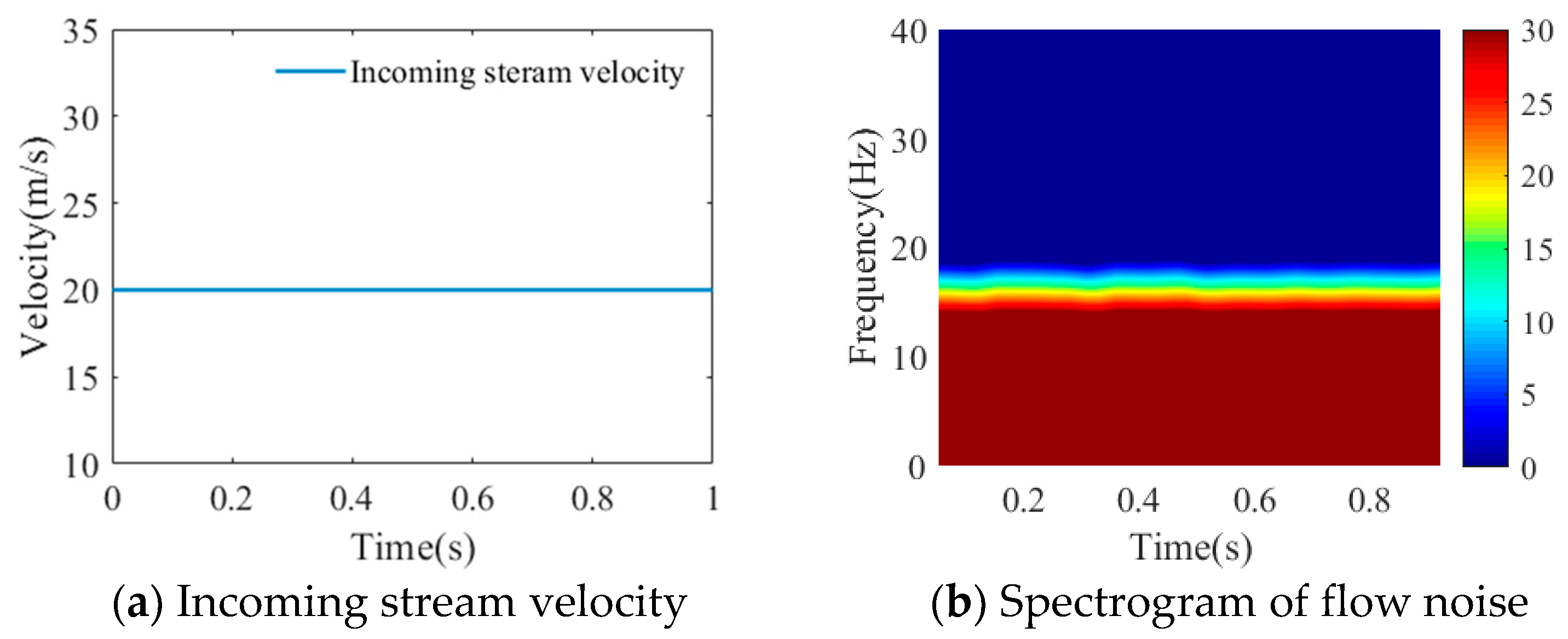
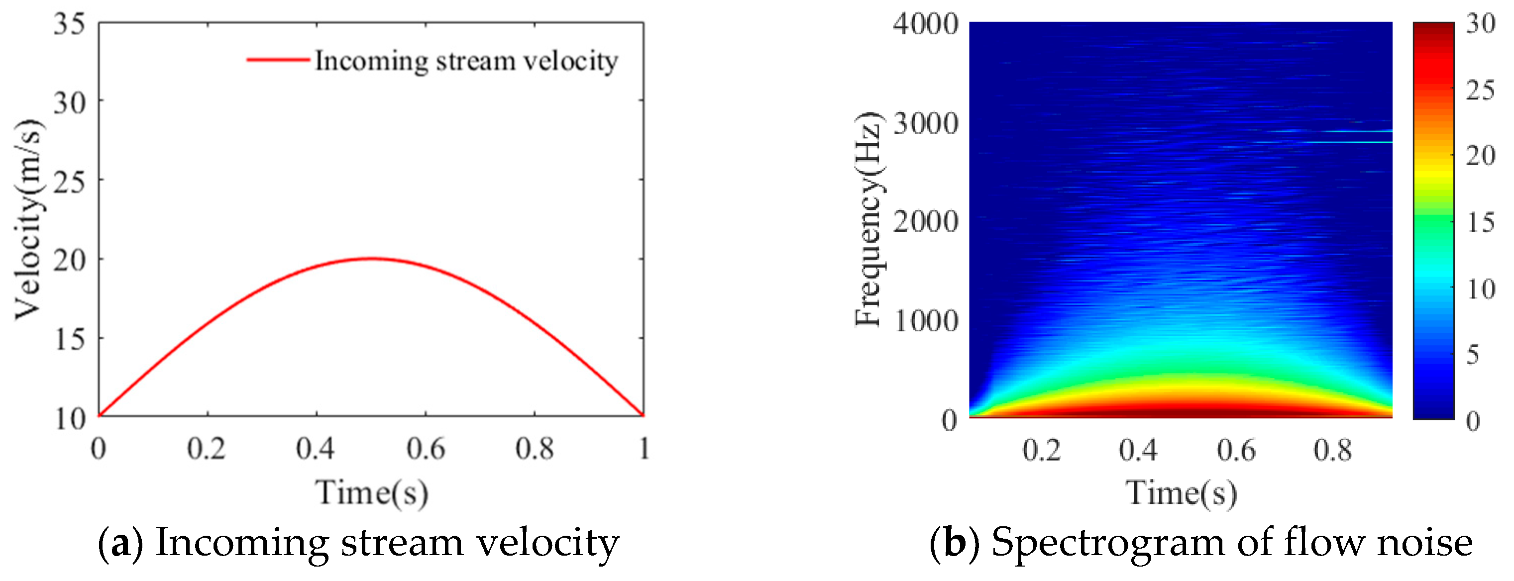
• Setting flow field calculation parameters. To obtain high-frequency flow noise, the time step is set to be 0.01 ms, the flow velocity of the inflow surface is 20 m/s, and the liquid density is 1000 Kg/m³.
• Computing the flow field. Ensuring calculation has converged by the two criterions: The residual of the calculation parameters decreases with the increase of iteration times and then tends to be stable; the values of observation points do not change with the number of iterations.
• Setting sound field calculation parameters’ boundary conditions. The reference sound pressure is 1 μPa, and the sound speed is 1500 m/s. The wall of the axisymmetric body is chosen as the noise source zone. The sound pressure receiver is set at the stagnation point.
• Computing the sound field. At first, the unsteady flow field is computed by solving the NS equations. Then, the FW-H integration approach is used to calculate the sound field.

The performance of the numerical calculation method is verified by the theoretical, analytical calculation method given above. The pressure coefficient of the surface of the axisymmetric body calculated by the numerical method is verified by the panel method. The numerical calculation result of flow noise is verified by the result calculated by the analytical calculation method.

The surface (XY section) pressure coefficient distribution of the axisymmetric body calculated by the finite element method is shown by the solid red line in Figure 2b. It can be seen that the numerical calculation result is in good agreement with the analytical result, which was calculated by the panel method. The power spectrum of the flow noise at the stagnation point calculated by the numerical method is represented by the red dotted line in Figure 4. It is indicated that the numerical result is in good agreement with the flow noise power spectrum obtained by the analytical expression.

The actual underwater environment is very complex. To overcome the difference between buoyancy and gravity during navigation, there will be an angle of attack between the axisymmetric body and its course. It can result in a certain angle between the incoming flow direction and the axis of the axisymmetric body. The flow field, radiation noise field, and power spectrum under different motion attitudes are analyzed below. The flow noise calculation process is the same as above, but the incoming stream velocity and the attitude of the axisymmetric body will be changed.

In Figure 6, (A) shows that the motion direction of the axisymmetric body which is consistent with its axis direction, (B) indicates that there is an angle of 10° between the motion direction of the axisymmetric body and its axis, and (C) shows that there is an angle of 10° between motion direction of the axisymmetric body and its axis. Here, the clockwise direction is taken as the positive direction.

Figure 7a shows the surface pressure coefficient distribution of the axisymmetric body in attitude A, and Figure 7b is the velocity field distribution corresponding to the attitude A. It is indicated that the pressure coefficient and the velocity field of the axisymmetric body in this attitude remain symmetric along the axis direction of the axisymmetric body, as shown in Figure 7a,b. Figure 7a indicates the surface pressure coefficient is largest at the stagnation point of the head of the axisymmetric body; it gradually decreases to a negative pressure along the curved surface of the head and then quickly returns to a positive pressure; this area is the transition region of the axisymmetric body. In this area, the pressure gradient is large, and the flow is very unstable. The radiated noise received of the acoustic array in the head mainly comes from this area. Figure 7b shows that the velocity of the flow field of the transition region is larger than that on the other parts of the axisymmetric body.

Figure 7c shows to the pressure coefficient distribution of the surface of the axisymmetric body under attitude B, and Figure 7d shows the velocity field under attitude B. It shows that when there is a certain angle between the direction of incoming stream and the axis of the axisymmetric body, the pressure and velocity distribution are no longer axially symmetric along the axis.

In attitude B, the smallest pressure coefficient and the maximum velocity appear in the upper part of the head. It can also be seen that the maximum velocity on the head under attitude B is larger than that in attitude A. In attitude C, the smallest pressure coefficient on the head of the axisymmetric body is located in the lower half, and its maximum velocity also appears at this position. The maximum velocity on the head in attitude C is also larger than that in attitude A.

Figure 8a–c displays the radiated noise field of the axisymmetric body corresponding to the attitude A, B, and C, respectively. From Figure 8a, it can be seen that the radiated noise of the axisymmetric body is symmetrical along its axial direction, and the radiated noise mainly propagates outward along the direction perpendicular to the axis of the axisymmetric body. Figure 8b shows that the noise energy in the upper part of the axisymmetric body head becomes significantly larger than that of the other part of the head. Figure 8c shows that the noise in the lower half of the head of the axisymmetric body becomes significantly larger. The results are consistent with the pressure field and the flow field conclusions under the three attitudes analyzed above. It means that the flow noise energy generated is larger when the flow velocity change is much larger. In addition, if the radiated noise propagation direction, shown in Figure 8a, is taken as a reference, then it can be seen that in attitude B, the propagation direction of the radiated noise is rotated by 10° in a clockwise direction overall; in attitude C, the propagation direction of the radiated noise is rotated by 10° in a counterclockwise direction.

Figure 9 shows the power spectrums corresponding to the flow noise at the stagnation point of the axisymmetric body in three attitudes. The reference sound pressure is 1 μPa. It can be seen that the power spectrum of the flow noise at the stagnation point under attitudes B or C is larger than that under attitude A, but the difference is not significant. The results of the flow noise power spectrum are also consistent with the velocity field results that were analyzed above.

This is because when there is an angle of attack between the incoming stream direction and the axis of the axisymmetric body, like attitude B; it leads to a more obvious change in the gradient of the contact surface between the upper part of the head and the fluid. As a result, the pressure stream velocity changes in this area are more dramatically. Therefore, the flow noise energy generated is much larger.

The stream in the actual marine environment is complex; it causes the speed of relative motion between the axisymmetric body and seawater to be time-varying. Next, the flow noise at the stagnation point is simulated when the incoming stream velocity is constant or changes continuously with time.

Figure 10b shows a spectrogram of the flow noise at the stagnation point of the axisymmetric body when the incoming stream velocity is constant, wherein the incoming stream velocity is shown in Figure 10a. Figure 11b shows a spectrogram of the flow noise at the stagnation point of the axisymmetric body when the incoming stream velocity magnitude changes with time and the incoming stream velocity (maximum velocity 20m/s) is presented in Figure 11a. As can be seen from Figure 10b and Figure 11b, the energies of the flow noise are concentrated below 20 Hz and 2000 Hz, respectively. To clearly see the distributions of the flow noise energy, the display ranges of frequency for Figure 10b and Figure 11b are 0–40 Hz and 0–4000 Hz, respectively.

From Figure 10 and Figure 11, it can be seen that the energy of the flow noise at the stagnation point of the axisymmetric body is a function of the free stream velocity. The flow noise energy is highly correlated with the incoming flow velocity, which indicates that the spectrum level of the flow noise hardly changes with time when the incoming flow velocity is constant; when the velocity is time-varying, the intensity of the flow noise also changes with time. From Figure 11, it can be seen that when the velocity becomes larger, the energy of the flow noise also shifts to a higher frequency correspondingly. In addition, as seen from Figure 10, when the incoming stream velocity is constant, the energy of the flow noise is concentrated in a very low frequency band. Figure 11 indicates that when the incoming flow velocity changes with time, the energy of the flow noise is concentrated in a relatively wider frequency band, and the energy gradually decreases as the frequency increases and then tends to a stable value.

As seen from Figure 12, when the incoming flow velocity is time-varying, the vorticity intensity on the axisymmetric body is greater.

Figure 13 shows the flow noise power spectrums at the stagnation point of the axisymmetric body under different incoming stream velocity conditions. The reference sound pressure is 1 μPa. It can be seen that the flow noise energy generated when the incoming flow velocity changes with time is much higher than that generated when the flow velocity is constant. This is because when the stream velocity magnitude changes with time, there is a turbulent fluid in the flow itself. Therefore, the stream changes more dramatically.

5. Conclusions

The flow noise of the underwater axisymmetric body has two adverse effects. It propagates to the far distance as a target source and limits the performance of self-sonar. Therefore, the study on the physical features of the flow noise of the axisymmetric body in a complex environment has great significance. In this paper, a detailed analytical calculation theory model was given, which could provide a reference standard for numerical simulation. Using the numerical method, the physical features of the flow noise of an axisymmetric body in a complex oceanic environment were analyzed.

Some results are summarized as follows. (1) The flow noise power spectrum at the stagnation point of the axisymmetric body computed by the analytical method is in good agreement with that computed by numerical method. (2) The transition region of the head of the axisymmetric body will be significantly different in three motion attitudes; it will migrate with the change of the incoming stream direction, which is important for the sonar system design in the fore-body. (3) The radiation direction of the flow noise will rotate at the same angle with the change of the incoming stream direction. (4) When the stream velocity is time-varying, the flow noise energy generated in the transition region is significantly larger than that when the stream velocity is constant. (5) In addition, it can be found that there is a significant correlation between the intensity of the flow noise and the incoming flow velocity, which can be seen as a feature for noise reduction in acoustic array signal processing.

References

1. Liu, Y.M.; Li, Y.L.; Shang, D.J. The generation mechanism of the flow-induced noise from a sail hull on the scaled submarine model. Appl. Sci. 2019, 9, 106. [Google Scholar] [CrossRef]
2. Abshagen, J.; Nejedl, V. Towed body measurement of flow noise from a turbulent boundary layer under sea conditions. J. Acoust. Soc. Am. 2014, 135, 637–645. [Google Scholar] [CrossRef] [PubMed]
3. Crighton, D.G.; Dowling, A.P.; Williams, J.E.F.; Heckl, M.; Leppington, F.G. Flow Noise on Surfaces. In Modern Methods in Analytical Acoustics; Springer: London, UK, 2016. [Google Scholar]
4. Li, X.G.; Yang, K.D.; Wang, Y. The diffracted sound field from the transition region of an axisymmetric body in water. Chin. Phys. B. 2011, 20. (In Chinese) [Google Scholar] [CrossRef]
5. Li, X.G.; Yang, K.D.; Mang, Y.L. Flow-noise calculation using the mutual coupling between vulcanized rubber and the flow around in water. Chin. Phis. Lett. 2012, 29. [Google Scholar] [CrossRef]
6. Gao, J.; Wu, P.G.; Li, T.R. Optimization-based model reference adaptive control for dynamic positioning of a fully actuated underwater vehicle. Nonlinear Dyn. 2017, 87, 2611–2623. [Google Scholar] [CrossRef]
7. Jagadeesh, P.; Murali, K.; Idichandy, V.G. Experimental investigation of hydrodynamic force coefficients over AUV hull form. Ocean Eng. 2009, 36, 113–118. [Google Scholar] [CrossRef]
8. Skudrzy, E.A.; Haddle, G.P. Noise production in turbulent boundary layer by smooth and rough surfaces. J. Acoust. Soc. Am. 1960, 32, 19–34. [Google Scholar] [CrossRef]
9. Lauchle, G.C. Noise generated by axisymmetric turbulent boundary-layer flow. J. Acoust. Soc. Am. 1977, 61, 694–703. [Google Scholar] [CrossRef]
10. Lauchle, G.C. On the radiated noise due to boundary-layer transition. J. Acoust. Soc. Am. 1980, 67, 158–168. [Google Scholar] [CrossRef]
11. Lauchle, G.C. Flow noise scaling at the stagnation point of an axisymmetric body. J. Sound. Vib. 1992, 154, 568–572. [Google Scholar] [CrossRef]
12. Arakeri, V.H.; Satyanarayana, S.G.; Mani, K.; Sharma, S.D. Studies on scaling of flow noise received at the stagnation point of an axisymmetric body. J. Sound. Vib. 1991, 146, 449–462. [Google Scholar] [CrossRef]
13. Li, X.G.; Yang, K.D.; Wang, Y. The power spectrum and correlation of flow noise for an axisymmetric body in water. Chin. Phys. B. 2011, 20. [Google Scholar] [CrossRef]
14. Kim, J.; Park, I.R.; Van, S.H.; Kim, W.J. Calculation of Turbulent Flows around a Submarine for the Prediction of Hydrodynamic Performance. SOTECH. 2003, 7, 16–31. [Google Scholar]
15. Yao, H.L.; Zhang, H.X.; Liu, H.T.; Jiang, W.C. Numerical study of flow-excited noise of a submarine with full appendages considering fluid structure interaction using the boundary element method. Eng. Anal. Bound. Elem. 2017, 77, 1–9. [Google Scholar] [CrossRef]
16. Lighthill, M.J. On sound generated aerodynamically. 1. General theory. Proc. R. Soc. Lond. Ser. A. 1952, 211, 564–587. [Google Scholar]
17. Lighthill, M.J. On sound generated aerodynamically. 2. Turbulence as a source of sound. Proc. R. Soc. Lond., Ser. A. 1954, 222, 1–32. [Google Scholar]
18. Williams, J.E.; Hawkings, D.L. Sound generation by turbulence and surfaces in arbitrary motion. Philos. Trans. R. Soc. 1969, 264, 321–342. [Google Scholar] [CrossRef]
19. Farassat, F.; Succi, G.P. The Prediction of Helicopter Discrete Frequency Noise. Vertica 1983, 7, 309–320. [Google Scholar]
20. Farassat, F.; Brentner, K.S. Supersonic quadrupole noise theory for high-speed helicopter rotors. J. Sound Vib. 1998, 218, 481–500. [Google Scholar] [CrossRef]
21. Farassat, F.; Brentner, K.S. The acoustic analogy and the prediction of the noise of rotating blades. Theor. Comp. Fluid Dyn. 1998, 10, 155–170. [Google Scholar] [CrossRef]
22. Gross, A.; Jagadeesh, C.; Fasel, H. Numerical investigation of three-dimensional separation on axisymmetric bodies at angle of attack. In Proceedings of the 50th AIAA Aerospace Sciences Meeting Including the New Horizons Forum and Aerospace Exposition, Nashville, TN, USA, 9–12 January 2012. [Google Scholar]
23. Gross, A.; Kremheller, A.; Fasel, H. Simulation of flow over suboff bare hull model. In Proceedings of the 49th AIAA Aerospace Sciences Meeting Including the New Horizons Forum and Aerospace Exposition, Orlando, FL, USA, 4–7 January 2011. [Google Scholar]
24. Shi, Y.; Pan, G.; Huang, Q.G. LES-based numerical simulation of flow noise for UUV with full appendages. Adv. Mater. Res. 2013, 631–632, 879–884. [Google Scholar]
25. Ramesh, S.S.; Meng, L.K.; Cheong, K.B. On the prediction of self-noise due to supercavitating underwater vehicle moving at subsonic speed using boundary element approach. In Proceedings of the ECUA 2012 11th European Conference on Underwater Acoustics, Edinburgh, UK, 2–6 July 2012. [Google Scholar]
26. Liu, Q.M.; Gao, X. Research on the virtual reality of impact of appendages on the flow characteristics of submarines based on neural networks and CFD. Neural Comput. Appl. Mar. 2018, 29, 1293–1301. [Google Scholar] [CrossRef]
27. Gungor, E. Hydroacoustical investigation on an generic underwater vehicle using Lighthill-Curle. J. Fac. Eng. Archit. Gaz. 2019, 34, 1352–1364. [Google Scholar]
28. Lauchle, G.C. Transition noise-the role of fluctuating displacement thickness. J. Acoust. Soc. Am. 1981, 69, 665–671. [Google Scholar] [CrossRef]
29. Littell, H.S.; Eaton, J.K. Unsteady flowfield behind a vortex generator rapidly pitched to angle of attack. AIAA. J. Apr. 1991, 29, 577–584. [Google Scholar] [CrossRef]
30. Josserand, M.A.; Lauchle, G.C. Modeling the wavevector-frequency spectrum of boundary-layer wall pressure during transition on a flat plate. J. Vib. Acoust. 1990, 112, 523–524. [Google Scholar] [CrossRef]
31. Hess, J.L.; Smith, A.M.O. Calculation of potential flow about arbitrary bodies. Prog. Aerosp. Sci. 1967, 8, 1–138. [Google Scholar] [CrossRef]
32. Lee, C.S.; Young, K.G.; Lee, J.T. A potential-based panel method for the analysis of a two-dimensional super-or partially-cavitating hydrofoil. J. Ship. Res. 1992, 36, 168–181. [Google Scholar]
33. Huang, J.Q.; Zhang, Y.W. Fluid Mechanics for Torpedoes; Northwestern Polytechnical University Press: Xi’an, China, 1989. (In Chinese) [Google Scholar]
34. Hutter, K.; Wang, Y. Simple Solutions of Boundary Layer Equations. In Fluid and Thermodynamics. Advances in Geophysical and Environmental Mechanics and Mathematics; Springer: Cham, Switzerland, 2016. [Google Scholar]
35. Zhang, N.; Shen, H.; Tian, Y. Computation of wall pressure fluctuations and flow induced noise by large eddy simulation. J. Acoust. Soc. Am. 2012, 131, 3333. [Google Scholar]
Figure 1. Boundary layer of the axisymmetric body.
Jmse 07 00323 g001
Figure 2. Partial view of the axisymmetric body model and its corresponding pressure coefficient.
Jmse 07 00323 g002
Figure 3. The Granville method to determine the unstable point and the transition point.
Jmse 07 00323 g003
Figure 4. Flow noise power spectrum at the stagnation point of the head of the axisymmetric body.
Jmse 07 00323 g004
Figure 5. Computing domain.
Jmse 07 00323 g005
Figure 6. Different sailing postures caused by the complex oceanic environment.
Jmse 07 00323 g006
Figure 7. Surface pressure coefficient and velocity field of the axisymmetric body
Jmse 07 00323 g007
Figure 8. Radiated noise field corresponding to the flow noise of the axisymmetric body in different attitudes (center frequency is 30 kHz).
Jmse 07 00323 g008
Figure 9. Flow noise power spectrum at the stagnation point of the axisymmetric body in different attitudes.
Jmse 07 00323 g009
Figure 10. Constant incoming stream velocity and the corresponding spectrogram of flow noise.
Jmse 07 00323 g010
Figure 11. Inconstant incoming stream velocity and the corresponding spectrogram of flow noise.
Jmse 07 00323 g011
Figure 12. Vorticity of the axisymmetric body under different incoming flow conditions.
Jmse 07 00323 g012
Figure 13. Flow noise power spectrum under different inflow conditions.
Jmse 07 00323 g013