Abstract
A particular aspect of the maritime operations involves available weather intervals, especially in the context of the emerging renewable energy projects. The Black Sea basin is considered for assessment in this work, by analyzing a total of 30-years (1987–2016) of high-resolution wind and wave data. Furthermore, using as reference, the operations thresholds of some installation vessels, some relevant case studies have been identified. The evaluation was made over the entire sea basin, but also for some specific sites located close to the major harbors. In general, the significant wave heights with values above 2.5 m present a maximum restriction of 6%, while for the western sector, a percentage value of 40% is associated to a significant wave height of 1 m. There are situations in which the persistence of a restriction reaches a maximum time interval of 96-h; this being the case of the sites Constanta, Sulina, Istanbul or Burgas. From a long-term perspective, it seems that there is a tendency of the waves to increase close to the Romanian, Bulgarian, and Turkish coastal environments—while an opposite trend is expected for the sites located on the eastern side.
1. Introduction
Climate change is a reality, being expected to deteriorate the current situation in a fast rate, as the energy demand significantly increases in the future. This problem is not new, and has already been known since 1966, with the mention that at that moment, only the natural fluctuations of energy and mass were taken into account, without considering human intervention [1]. The marine environment is more sensitive to these natural changes and an increase of the wave action combined with the sea-level rise will significantly influence the dynamics of the coastal areas [2,3,4,5]. Some well-known weather patterns are already associated to the marine areas, this being the case of El Nino, La Nina or the Southern Oscillations [6,7].
At this moment, important attention is given to the long-term assessment of the wind and wave conditions by taking into account various climate scenarios. For example, in the work of Rusu [8] a complete assessment of the Black Sea wave energy was carried out by considering two-time intervals, namely 1976–2005 (historical data) and 2021–2050 (near future). The results show that in the near future, the wave power will increase in the western part of the Black Sea, with a maximum variation of 16% expected. On the opposite side, the south-eastern region may report a decrease of the average values with almost 9%. In a similar way, Hemer and Trenham [9] performed a global evaluation of the wave conditions under various scenarios, with emphasis on the importance of this topic from an economical and environmental point of view. In Lemos et al., [10] the time interval from 2031 to 2060 was considered for the investigation of the global wave climate. The results indicate two dominant trends; revealing the fact that some geographical regions are affected much faster by climate changes in the first half of the 21st century, while other important variations are expected for the last 40 years of this century. As for the wind conditions, recent studies suggest a possible increase of the wind power in the range 30–137% for the Black Sea [11], while at a global scale, a general decrease of the wind resources in Asia and Europe is expected, and an increasing trend for America [12]. By looking at the European large-scale wind resources (2016–2100), an increase of the resources only for the Baltic Sea (+ up to 30%) is expected, and a decrease of 30% for Eastern Europe. On a seasonal level, a decrease in summer and autumn (except the Baltic regions) is expected, while during wintertime the northern-central part of Europe will report an increase [13].
There is already growing interest for renewable projects, with significant progress in the case of the marine areas, where it is possible to implement large-scale generators. This is the case of the European offshore wind market that gradually rose from 500 MW (in 2008) until 18,499 MW at the end of 2018. A significant percentage of the wind parks include bottom-fixed foundations (jacket or monopile), but there is also a tendency to implement floating platforms, as in the case of Kincardine or Floatgen projects. Reported in the year 2018, there is some interest to implement wind projects in (semi) enclosed seas, this being the case of the North (62%), Irish (15%), and Baltic Sea (14%) while on the opposite side of the Atlantic Ocean is located with only 9% [14]. Beside these regions, some other important basins may become attractive for the implementation of an offshore project, from which we can mention the Mediterranean, Caspian or Black seas [15,16,17].
Compared to the onshore sites, the marine areas present particular environmental conditions that significantly influence the successful development of a project. More precisely, the available weather windows represent an important element that needs to be taken into account, since around these intervals, an entire supply chain is concentrated that involves economical or logistical aspects. Similar research was covered in O’Connor et al. [18], where the Irish west coast wave conditions were considered for assessment. As indicated, a planned maintenance program would be more efficient than to repair a device on-site, or eventually to disconnect and transport to a shore base. According to these results, for a site located approximately 74 km offshore; an annual accessibility window of 2% (for significant wave heights < 1 m) was indicated; of 13% (for significant wave heights < 1.5 m); 28% (for significant wave heights < 2 m) or 45% (for significant wave heights < 2.5 m). The same area was considered for analysis in Gallagher et al. [19], in this case, the wind conditions were also taken into account. Per total, the accessibility of the south coast is much lower than on the east coast, especially during the winter, when this can drop until 50% and the maximum waiting time can exceed 18 days. In Silva and Estanqueiro [20], special attention was given to the coast of Portugal, where the environmental conditions related to some theoretical offshore wind farm were discussed. Various combinations of significant wave height and wind speed were considered, the lowest accessibility value (below 40%) being reported for a rubber boat during the interval from March to May and from December to February, respectively. In a similar way, various scenarios were discussed for different areas such as the North Sea [21,22], Barents Sea [23] or the Japan coastal area [24].
In this context, the following research questions will guide the present work:
- (a)
- What is the spatial distribution of the adverse weather windows reported for the Black Sea?
- (b)
- For this geographical environment, how many windows of restricted weather may occur?
- (c)
- What is the long-term profile of the adverse weather events?
2. Materials and Methods
2.1. Target Area
The Black Sea has an area of 423,000 km2 and a maximum depth of 2258 m. With a total coastline length of 4125 km, this basin is divided between Bulgaria, Turkey, Georgia, Russia, Ukraine, and Romania [25]. In order to assess the distribution of the adverse weather intervals, some important harbor areas were taken into account, as seen in Figure 1 and Table 1. For the present work, these sites are defined approximately 30 km offshore, in order to cover a full range of maritime activities, including the development of an offshore wind project [16].
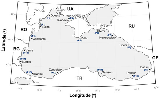
Figure 1.
The locations of the reference points selected for the Black Sea coastal environment.

Table 1.
Locations of the considered sites (P1–P15).
2.2. Wind and Wave Data
The wind data used in the present work are produced by the U.S. National Centers for Environmental Prediction—Climate Forecast System Reanalysis (further denoted with NCEP), and cover a 30-year time interval (1987–2016). In this case, a dataset that is defined by a spatial resolution of 0.32 degree was processed, for which eight values per day were extracted for a 3 h time step (0-3-6-9-12-15-18-21 UTC - Coordinated Universal Time). These wind fields are defined by a reference height of 10 m and therefore the wind speed is U10. The selection of the NCEP data was made based on some previous studies that highlight the accuracy of this model. In Sharp et al. [26] the wind conditions from the United Kingdom (onshore and offshore) were evaluated and encountered a good agreement between the NCEP data and in situ measurements. Akpinar et al. [27] considered this wind data to run a wave model focused on the Black Sea, the results indicating a strong connection between the water depth and wind speed. More details regarding the technical aspects and the assembly of the NCEP dataset can be found in Saha et al. [28].
The same NCEP wind fields above mentioned were used to drive the Simulating Waves Nearshore [29] (SWAN) model in order to simulate the sea state conditions over the 30-year period considered. The computational domain of the SWAN model is a regular grid with a resolution of 0.08 degrees (175 cells in longitude and 75 cells in latitude) and it coincides with the bathymetric grid. The lower left corner (27.5°E/41.0°N) represents the origin of the computational domain. The simulations were carried out in the non-stationary mode with a time step of 10 min, considering in the spectral space, 36 directions and 30 frequencies (ranging between 0.05 and 1.0 Hz). All the wave model settings considered in the present work are those used in previous studies performed in the Black Sea area [30,31,32,33]. The SWAN model results were validated against in-situ and satellite measurements [30,31]. Moreover, the accuracy of the wave model results was also evaluated under storm conditions [32]. In all the studies mentioned above, the wave modeling system based on SWAN forced with the NCEP wind fields was shown, as considered in the present work and provides reliable results in the Black Sea basin.
2.3. Case Studies
Several scenarios will be considered for evaluation, as can be observed from Table 2. These criteria were proposed by Kikuchi and Ishihara [24] and cover all the operations required to develop an offshore wind project. Two different scenarios are identified: scenario A—only wave conditions; scenario B—combined wind and wave action. The first scenario involves the bottom preparation and the substrucure assembly, which means that only the wave heights located below 1.25 m are considered to be representative. In the final part of the project, which involves among other installation of the blades, a maximum significant wave height (Hs parameter) of 2.5 m and a U10 value of 10 m/s can be considered as maximum threshold. In this work, we consider the marine conditions above these limits, in order to identify the restricted weather intervals during which no activity will be possible.
Table 2.
Operational limits reported for different stages of an offshore wind project [24].
3. Results
3.1. Spatial Distribution of the Adverse Weather Windows
Figure 2 provides a first perspective of the Hs distribution, by taking into account only the significant wave heights above 1 m and 2.5 m, respectively. As expected, the central part of the sea is defined by higher values. This geographical environment is defined by two distinct areas, located in the west and east. The conditions reported in the western part are much higher, this aspect being more visible in the case of the Hs values above 1 m/s, for which a maximum of 40% is noticed. These values decrease in the vicinity of the coastline, a distribution in the range of 20–28% expected for the western regions, while in the east the values can go up to 24%. A smoother distribution is noticed for the 2.5 m threshold, where the values located between 4% and 6% are dominant in the west, compared to the interval 0–2% that may be noticed in the east.
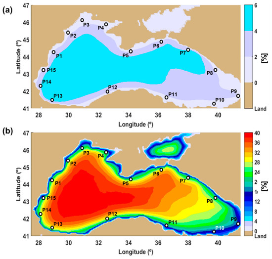
Figure 2.
The spatial distribution of the significant wave height (Hs), as resulted from the 30-year Simulating Waves Nearshore (SWAN) simulations (1987–2016). Results reported for: (a) Hs > 2.5 m (in %); (b) Hs > 1 m (in %).
A more detailed assessment of the wave conditions is provided in Figure 3, considering this time the seasonal distribution of the Hs values above 1 m. Four main seasons were considered, as follows: (a) winter—December/January/February; (b) spring—March/April/May; (c) summer—June/July/August; (d) autumn—September/October/November. During the winter time, the maritime activities are limited in almost 60% of the time (offshore areas), a minimum of 30% in the case of the coastal areas from the south–east expected. More energetic conditions can also occur during autumn, when the western part of the Black Sea indicates adverse weather windows in the range 28–44%. The best season to initiate a project is during the summer, when it is possible to have no adverse windows, especially in the case of the regions located close to the Turkish coast (in the south–west).
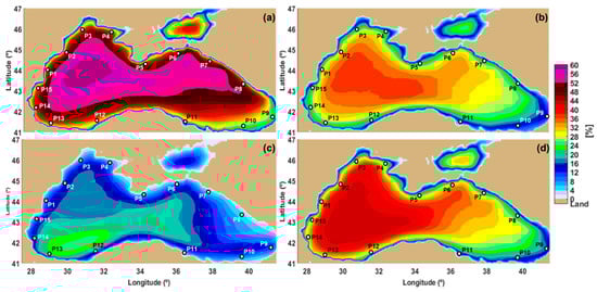
Figure 3.
Seasonal distribution of the Hs parameter higher than 1 m considering the entire 30-year SWAN simulations (1987–2016), where: (a) winter; (b) spring; (c) summer; (d) autumn.
Going to the higher wave conditions, the seasonal distribution by using an Hs value of 2.5 m is presented in Figure 4, as a reference. During spring and summer, there is almost no restriction from this point of view, especially in the case of the coastal areas. These values decrease in the case of autumn, with a maximum restriction of 8% in the south-western areas, while in the vicinity of the shoreline a maximum limitation of 4% is noticed. In the case of the winter season, two hot-spots (south-west and north-east) of 14% are more visible, with the mention that in the Azov Sea the weather conditions will have no influence on the maritime operations.
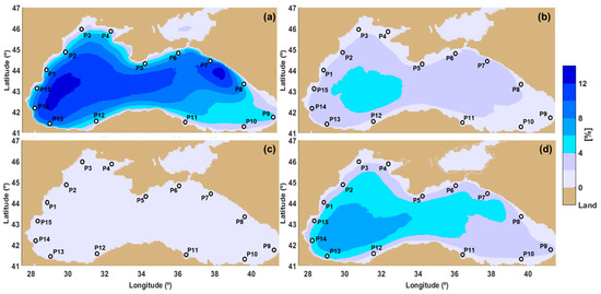
Figure 4.
Seasonal distribution of the Hs parameter higher than 2.5 m considering the entire 30-year SWAN simulations (1987–2016), where: (a) winter; (b) spring; (c) summer; (d) autumn.
In the case of the NCEP wind data, a first perspective is provided in Figure 5, from which we notice that the Azov Sea represents an interesting area in terms of the wind resources, reporting higher conditions than in the Black Sea. From the evaluation of the map associated to the value of 10 m/s, we can notice that a maximum restriction of 24% is accounted by the Azov Sea while 20% is noticed in the western part of the Black Sea. For the sites located in the south-east (Batumi-Trabzon-Samsun), the restricted conditions are quite low reaching a maximum of 4%. A different picture corresponds to the 6 m/s threshold, this value being mentioned in the assembly process of an offshore wind turbine. A mixture of wind fields occurs, the central and western regions reporting values that exceed 40% and reaching a maximum of 64% near the Azov Sea. As for the eastern regions, the workability is higher, reaching a maximum of 32% in the offshore area and values close to 16% close to the shoreline. At this point, we can mention that in general, the eastern part seems to be defined by lower adverse conditions (U10 parameter), that may indicate that an offshore wind project does not represent a suitable solution for this area.
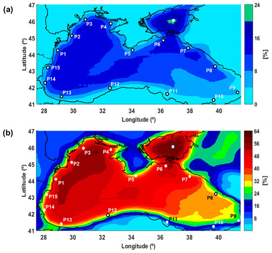
Figure 5.
The spatial distribution of the wind speed, considering the entire 30-year period (1987–2016) of NCEP data. Results reported for: (a) U10 > 10 m/s (in %); (b) U10 > 6m/s (in %).
Figure 6 presents the seasonal distribution of the wind speed, using as a reference a U10 value of 6 m/s. In all cases, the Azov Sea indicates the highest distribution that goes from 72% in winter to 40% during summer. Also close to the Kerci site, a hot spot that shows higher restrictions can be noticed. During winter, the operations will be limited by at least 50% in the case of operations carried out in the western part and by maximum 40% for the offshore operations associated to the eastern side. Close to the shore, a minimum of 24% is expected in the case of the sites Trabzon and Samsun, respectively. Higher restrictions are also expected during the autumn, when the workability is limited by at least 40%, an exception being the eastern part, where the values can drop below 36%. During the summer time there are some regions, which stand out in terms of the restricted conditions, but in general, the values do not exceed 36%. From the analysis of the wind distribution (onshore and offshore), it seems that the water areas are defined by significantly higher resources.
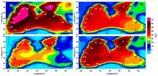
Figure 6.
Seasonal distribution of the U10 parameter higher than 6 m/s considering the entire 30-year period (1987–2016) of NCEP wind data, where: (a) winter; (b) spring; (c) summer; (d) autumn.
A similar evaluation is provided in Figure 7, taking this time as reference a wind speed of 10 m/s. The winter and autumn seasons stand out with more impresive values that can reach around 32% in the Azov Sea and a maximum of 28% in the western part of the Black Sea. Spring is defined by a maximum of 16% (Azov Sea) also noticed some hotspots in the north-west and also in the area located between Zonguldak and Samsun. According to this scenario, summer seems to be the most accessible season being noticed adverse windows in the range 4–8% close to the shoreline, while a maximum value of 10% is accounted by the Azov Sea.
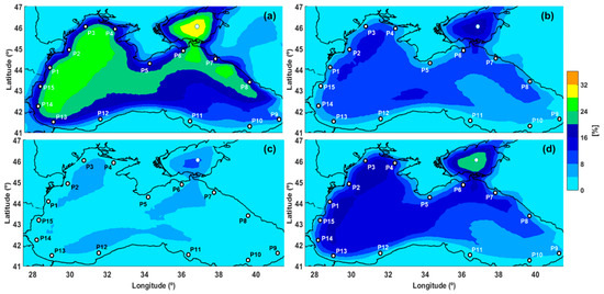
Figure 7.
Seasonal distribution of the U10 parameter higher than 10 m/s considering the entire 30-year period (1987–2016) of NCEP wind data, where: (a) winter; (b) spring; (c) summer; (d) autumn.
3.2. Assessment of the Weather Windows Close to the Harbour Areas
Beside the spatial distribution of the adverse conditions, another objective of this work is to identify the adverse weather profiles of the sites indicated in Table 1 by taking into account the wind and wave criteria mentioned in Table 2. In order to present these results in a concise way, in Table 3, the top five sites were identified. These were sorted from the highest to the lowest values. Regardless of the scenario taken into account (wind or wind+wave), the same sites are presented, being noticed small differences between their positions. Maximum values are accounted by the sites P14, P13, P2/P6 being also reported notable values for the sites P4 and P7, but only for the wind and wave selection.
Table 3.
Top five sites reporting the highest adverse weather conditions.
Figure 8a illustrates the variation of these values, by taking into account only the wave characteristics. The values significantly decrease as we go from the 0.5 m threshold to the 1.25 m threshold, when values between 9.26% and 72.83% can be encountered. Much higher values are noticed close to the sites P1, P2, P6, and the group P12–P15, compared to the sites P9–P11 that indicate a limited number of adverse weather events. In Figure 8a, the wind speed was also considered. In this case, the values reported for the criteria Hs > 2.5 m and U10 > 10 m/s indicate a similar pattern as the ones reported for Hs > 2.5 m and U10 > 8 m/s. The maximum values correspond to the combination Hs > 1 m and U10 > 6 m/s, when there are expected values of 27.93% for the site P2, 24.66% for P6 and a constant decrease until 5.89% for P11, which is followed by an increase until 28.06% (P14).
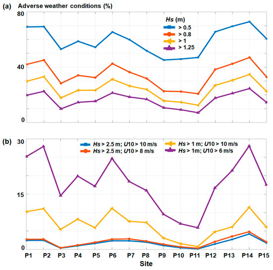
Figure 8.
Adverse weather conditions (in %) reported by the reference sites, considering the time interval from 1987 to 2016, where: (a) wave conditions; (b) joint distribution of the wind and wave conditions.
Figure 9 presents the monthly distribution, taking into account only two environmental conditions (Hs > 1.25 m; Hs > 2.5 m and U10 > 10 m/s). The background of the highest values is represented in red while the lowest values are marked in white.
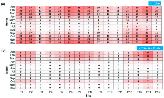
Figure 9.
Monthly distribution of the adverse weather conditions (in %) reported for: (a) Hs > 1.25 m; (b) Hs > 2.5 m and U10 > 10 m/s.
According to the Hs distribution (Figure 9a), it is possible to see a clear distinction between the months January, February, March, October, November, December (6 months), and the rest of the year, the mentioned ones showing much higher values. Maximum restrictions of 41% correspond to the sites P6 and P14, compared to a minimum value of 2% that represents a common event for the site P11, especially during the summer time. A significant percentage of the interval May–August is defined by values that do not exceed 10%, being also reported a maximum of 18% in the case of the site P13. As for the joint distribution of the wind and waves (Figure 9b), in fact, a 10% restriction represents a not so common distribution being reported only by P14 in February. Since most of the values are close to zero, we can conclude that the maritime operations related to this threshold will have little restrictions, regardless of the season considered.
By including the number of adverse weather occurrences, it is possible to provide a complete profile of the adverse weather events. Figure 10 provides such analysis by considering some case studies (average values per year), and also different time intervals such as 6 h, 24 h or 96 h, respectively. As expected, the shorter time intervals indicate the highest number of occurrences that can go up to 108 annual events in the case of the conditions reported above 0.5 m. For the significant wave heights higher than 1.25 m, there are higher variations of the values being expected maximum 65 events for the site P2 (6-h interval) and around one or two events for the conditions that cover 96 h.
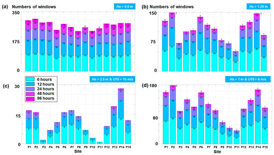
Figure 10.
Number of windows reported above a particular threshold, where: (a) Hs > 0.5 m; (b) Hs > 1.25 m; (c) Hs > 2.5 m and U10 > 10 m/s; (d) Hs > 1 m and U10 > 6 m/s.
A maximum of 13 events for the 6-h interval and nine events for the 12-h interval are expected for the wind and wave conditions above 2.5 m and 10 m/s (Figure 10c), these values being related to P14. For the long-term operations (≥ 24 h), the number of events falls in the interval of one to five occurrences per year. As we lower the wind and wave threshold (Figure 10d), the number of restrictions significantly increases to maximum 13 events for the 48-h interval. Table 4 presents a top five of the sites defined by the longest sequences of adverse weather windows. If we only consider the waves, the site P2 and P14 account for the first positions, being also reported a significant presence of the sites P1, P6 and P13. For the wind/waves scenarios, there is no clear pattern from this point of view, being expected more sequences that are frequent close to the sites P1, P12, P13 and P14, respectively.
Table 4.
Top five sites reporting the longest sequences of adverse weather conditions.
3.3. Inter-Annual Variability of the Adverse Conditions
Figure 11 presents the annual evolution of the weather conditions taking into account only the significant wave heights. According to the linear trend reported for Constanta (Figure 11a) there is a tendency of the wave heights higher than 0.5 m to decrease, while for the waves above 1.25 m it is expected an increase. For this site several peaks are noticed, maximum of 76% (Hs > 1.25 m) in the interval 1997 and 2002, while minimum values of 14% (Hs > 0.5 m) and 62% (Hs > 1.25 m) are related to the time interval 1987 and 1992.
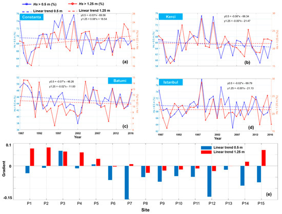
Figure 11.
Inter-annual distribution of the Hs parameter, where: (a–d) evolution of the wave heights higher than 0.5 m and 1.25 m reported for the Constanta, Kerci, Batumi and Istanbul sites; (e) gradient distribution for all the reference sites.
For the Kerci site, a slight decrease of the significant wave heights is observed, the minimum and maximum peaks being similar to the ones from Constanta site. In addition, the Batumi site shows a reduction of the significant wave heights and a possible explanation is that the values from the period 1992 and 2002 influence this trend, being reported much lower values. Compared to the other two sites, much smaller values are noticed, reaching a value of 12.9% (Hs > 1.25 m) or 47.33% (Hs > 0.5 m) for the year 2016. In the case of Istanbul, the variation is more visible for the waves above 0.5 m, being reported restrictions in the range 15–20% (Hs > 0.5 m) or 62–78% (Hs > 1.25 m), respectively. In Figure 11e, the gradient distribution of all the sites is presented, a positive value indicating an increase of the adverse conditions. According to these values, an increase of the wave height only in the case of the sites located in the western part of the Black Sea (Bulgaria, Romania and Ukraine) is encountered, while a strong decrease of the adverse conditions is close to P7 and P12, but only for the waves that exceed 0.5 m.
Figure 12 presents a similar analysis, including also the wind conditions. The gradient values associated to the sites Kerci and Istanbul, indicate a gradual decrease for the interval 2002 and 2016. The Batumi site does not show a clear pattern, while in the case of Constanta it is more likely that the adverse conditions to increase in magnitude. For the first case study (Hs = 1 m and U10 = 6 m/s) the annual value oscillates between 22% and 34% (Constanta); 10% and 40% (Kerci); 7% and 16% (Batumi); 12% and 32% (Istanbul). For the second scenario, the restricted interval does not exceed 6%. From the gradient distribution (Figure 12e) it is clear that most of the sites are defined by a decrease, the values corresponding to the sites P6 and P7 being substantially higher.
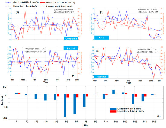
Figure 12.
Inter-annual distribution of the wind and wave conditions, where: (a–d) annual values and linear trends reported for the Constanta, Kerci, Batumi and Istanbul sites; (e) gradient distribution for all the reference sites.
Figure 13 shows the number of sequences defined by a 6-h time step, considering all the reference sites. The group sites P1–P4 present a relatively similar distribution, while much higher values are noticed in the site P2. On the other hand, a minimum of 20 events is accounted by P3, which also indicates a long-term increase of these intervals. For the next group of points (P5–P8), the number of sequences seems to reduce overtime, being also expected peaks of 78 events in the case of P6. The site P12 presents higher values than P10–P12, reaching maximum 70 events, while on the opposite side we found P11 with a minimum value of 15 events for the year 1996. Maximum of 82 events are accounted by the site P14 in the interval 1996 and 2001, being also noticed time intervals where there is no fluctuation between the values.
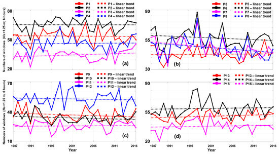
Figure 13.
The number of windows of 6 h above 1.25 m threshold, where: (a) P1–P4 sites; (b) P5–P8 sites; (c) P9–P12 sites; (d) P13–P15 sites.
Figure 14 illustrates the variations of the adverse windows events (6-h interval) by taking into account a significant wave height of 2.5 m and a wind speed of 10 m/s. The restricted period seems to increase in the case of the sites P1, P9, P12 and P15, while the group sites P5–P8 reports a decrease.
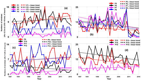
Figure 14.
Number of windows of 6 h above 2.5 m (Hs) and 10 m/s (U10) threshold, where: (a) P1–P4 sites; (b) P5–P8 sites; (c) P9–P12 sites; (d) P13–P15 sites.
The values do not exceed 25 events per year, being also expected no restrictions, as in the case of the site P11 or for the sites P7 and P8, that indicates lower occurrences during the interval 2011 and 2016.
4. Conclusions
The assessment of the adverse weather conditions represents an important aspect that can contribute to the success of a marine project, especially if we discuss about a renewable one. Since the Black Sea is an enclosed basin, the marine conditions are less aggressive than in the case of the ocean areas, in particular, if we discuss about waves. In the existing literature, there are two ways to analyze these conditions, either by considering an availability interval or on the contrary to identify restrictions, during which no activity will be possible. For the offshore wind farms several Hs limits seem to emerge as in the case of the personal transfer by boats or single hulled vessels, which are located in the range 1.5–2 m. For the multihull vessels or Ampelmann transfer system, these values can increase up to 2.5 m or 3 m. For example, in the case of an offshore wind farm located in the North Sea (45 km of the coast), the level of access increases from 34% (Hs = 0.75 m) to almost 95% (Hs = 3 m). In this case, it is possible that the level of access to decrease by a maximum value of 9%, as we go from the nearshore to offshore (100 km) [18]. Besides the availability issues, the cost required to rent installation vessels (per day) is quite high, some examples are given as follows: jack-up barge 100,000 to180,000$; crane barge—80,000 to100,000$; cargo barge—30,000 to 50,000$; tug boat—1000 to 5000$. The complete assembly of an offshore wind farm may vary from 1.5 months (the Alpha Venus project) up to 11 months (the Princess Amalia project), according to the number of the turbines installed [34]. If we discuss about the existing offshore wind projects, it is possible to identify some maintenance time required to carry various activities, such as: inspection—3 h; minor/major repair—3 to 10 h; partial replacement—50 h; complete replacement—70 h [35].
In this work, we consider assessing the Black Sea restricted weather intervals by taking into account, a joint distribution of the wind and wave conditions, coming from high-resolution numerical models. From the knowledge of the authors, there are no such studies focused on this topic, one of the main reasons being that at this moment there is no interest to develop offshore wind farms in this marine environment, although there are suitable wind resources [15,17]. From the analysis of the maps representing the spatial distribution of the wind and wave conditions, it was highlighted the fact that the western part of the Black Sea is defined by more restrictions, that can go up to 60% in the case of the winter season (Hs > 1 m). On a regional scale, the wind maps suggest that in fact much higher wind resources correspond to the Azov Sea. On the other hand, in the Black Sea the sites located close to the Romanian, Bulgarian and Turkish waters present the highest number of adverse windows, that can go up to 30% in the case of the joint distribution of the wind and waves (Hs > 1 m; U10 > 6 m/s). The number of restricted events that exceeds 24 h is quite limited for the systems operating below Hs values of 2.5 m, being expected higher values for the systems operating below 0.5 m. This is the case of the site Sulina with 108 annual events (6-h); 84 events (12-h); 60 events (24-h); 38 events (48-h) or 18-events (96-h).
Another objective of this work was to identify the long-term fluctuations of the adverse events, taking into account that a 30-year period (1987–2016) of data was processed. Some case studies were selected and different patterns have been identified. Thus, it seems that the waves that exceed 0.5 m decrease in general, being expected a clear increase close to the site Odessa. Going to the Hs values of 1.25 m, there is a clear increase reported by the sites Constanta Sulina, Odessa, Skadovsk and Yalta and Varna. When the wind conditions were also considered, more clear variations are accounted by the sites Kerci and Novorossiysk, being noticed a decrease of the marine conditions (Hs > 1 m; U10 > 6 m/s).
Finally, according to the present results, we can conclude that the Black Sea is a favourable environment for the development of a marine project, such as an offshore wind farm, with suitable marine conditions for the maritime operations. The best seasons to initiate a project are spring and summer, while for the sites located in the western sector the winter season is not a suitable one. The enclosed seas represent suitable areas for the development of the wind farms, and probably that in the near future there are higher chances to implement such projects close to the Romanian and Bulgarian coastal waters.
Author Contributions
F.O. performed the literature review, carried out the statistical analysis and assembly the manuscript. L.R. guided this research, processed the dataset and produced the spatial maps. All the authors approved the final manuscript.
Funding
This work was supported by a grant of Ministery of Research and Innovation, CNCS-UEFISCDI, project number PN-III-P1-1.1-PD-2016-0235, within PNCDI III.
Acknowledgments
The CFSR data were developed by NOAA’s National Centers for Environmental Prediction (NCEP). The data for this study are from the Research Data Archive (RDA) which is maintained by the Computational and Information Systems Laboratory (CISL) at the National Center for Atmospheric Research (NCAR). NCAR is sponsored by the National Science Foundation (NSF). The original data are available from the RDA (http://dss.ucar.edu) in dataset number ds093.2.
Conflicts of Interest
The authors declare no conflict of interest.
Nomenclature
| U10 | wind speed reported at 10 m above sea level |
| SWAN | Simulating WAves Nearshore |
| NCEP | NOAA’s National Centers for Environmental Prediction |
| Hs | significant wave height |
References
- Mitchell, J.M., Jr.; Dzerdzeevskii, B.; Flohn, H.; Hofmeyr, W.L.; Lamb, H.H.; Rao, K.N.; Wallen, C.C. Climatic Change: Report of a Working Group of the Commission for Climatology; Technical Note No. 79; World Meteorological Organization (WMO): Geneva, Switzerland, 1966. [Google Scholar]
- Bonaduce, A.; Staneva, J.; Behrens, A.; Bidlot, J.-R.; Wilcke, R.A.I. Wave Climate Change in the North Sea and Baltic Sea. J. Mar. Sci. Eng. 2019, 7, 166. [Google Scholar] [CrossRef]
- Erikson, L.; Barnard, P.; O’Neill, A.; Wood, N.; Jones, J.; Finzi Hart, J.; Vitousek, S.; Limber, P.; Hayden, M.; Fitzgibbon, M.; et al. Projected 21st Century Coastal Flooding in the Southern California Bight. Part 2: Tools for Assessing Climate Change-Driven Coastal Hazards and Socio-Economic Impacts. J. Mar. Sci. Eng. 2018, 6, 76. [Google Scholar] [CrossRef]
- Rute Bento, A.; Rusu, E.; Martinho, P.; Guedes Soares, C. Assessment of the changes induced by a wave energy farm in the nearshore wave conditions. Comput. Geosci. 2014, 71, 50–61. [Google Scholar] [CrossRef]
- Rusu, E.; Macuta, S. Numerical Modelling of Longshore Currents in Marine Environment. Environ. Eng. Manag. J. 2009, 8, 147–151. [Google Scholar] [CrossRef]
- Jury, M.R. Global wave-2 structure of El Niño–Southern Oscillation-modulated convection. Int. J. Climatol. 2019, 39, 2438–2448. [Google Scholar] [CrossRef]
- Kim, K.-Y.; Kim, Y.Y. Mechanism of Kelvin and Rossby waves during ENSO events. Meteorol. Atmos. Phys. 2002, 81, 169–189. [Google Scholar] [CrossRef]
- Rusu, L. Evaluation of the near future wave energy resources in the Black Sea under two climate scenarios. Renew. Energy 2019, 142, 137–146. [Google Scholar] [CrossRef]
- Hemer, M.A.; Trenham, C.E. Evaluation of a CMIP5 derived dynamical global wind wave climate model ensemble. Ocean Model. 2016, 103, 190–203. [Google Scholar] [CrossRef]
- Lemos, G.; Semedo, A.; Dobrynin, M.; Behrens, A.; Staneva, J.; Bidlot, J.-R.; Miranda, P.M.A. Mid-twenty-first century global wave climate projections: Results from a dynamic CMIP5 based ensemble. Glob. Planet. Chang. 2019, 172, 69–87. [Google Scholar] [CrossRef]
- Rusu, E. A 30-year projection of the future wind energy resources in the coastal environment of the Black Sea. Renew. Energy 2019, 139, 228–234. [Google Scholar] [CrossRef]
- Zhang, F.; Wang, C.; Xie, G.; Kong, W.; Jin, S.; Hu, J.; Chen, X. Projection of global wind and solar resources over land in the 21st century. Glob. Energy Interconnect. 2018, 1, 443–451. [Google Scholar]
- Carvalho, D.; Rocha, A.; Gómez-Gesteira, M.; Silva Santos, C. Potential impacts of climate change on European wind energy resource under the CMIP5 future climate projections. Renew. Energy 2017, 101, 29–40. [Google Scholar] [CrossRef]
- Offshore Wind in Europe—Key Trends and Statistics 2018. Available online: https://windeurope.org/about-wind/statistics/offshore/european-offshore-wind-industry-key-trends-statistics-2018/ (accessed on 8 March 2019).
- Onea, F.; Rusu, E. Efficiency assessments for some state of the art wind turbines in the coastal environments of the Black and the Caspian seas. Energy Explor. Exploit. 2016, 34, 217–234. [Google Scholar] [CrossRef]
- Onea, F.; Rusu, E. An Assessment of Wind Energy Potential in the Caspian Sea. Energies 2019, 12, 2525. [Google Scholar] [CrossRef]
- Onea, F.; Rusu, L. Evaluation of Some State-Of-The-Art Wind Technologies in the Nearshore of the Black Sea. Energies 2018, 11, 2452. [Google Scholar] [CrossRef]
- O’Connor, M.; Lewis, T.; Dalton, G. Weather window analysis of Irish west coast wave data with relevance to operations 82 maintenance of marine renewables. Renew. Energy 2013, 52, 57–66. [Google Scholar] [CrossRef]
- Gallagher, S.; Tiron, R.; Whelan, E.; Gleeson, E.; Dias, F.; McGrath, R. The nearshore wind and wave energy potential of Ireland: A high resolution assessment of availability and accessibility. Renew. Energy 2016, 88, 494–516. [Google Scholar] [CrossRef]
- Silva, N.; Estanqueiro, A. Impact of Weather Conditions on the Windows of Opportunity for Operation of Offshore Wind Farms in Portugal. Wind Eng. 2013, 37, 257–268. [Google Scholar] [CrossRef]
- Wolken-Möhlmann, G.; Bendlin, D.; Buschmann, J.; Wiggert, M. Project Schedule Assessment with a Focus on Different Input Weather Data Sources. Energy Procedia 2016, 94, 517–522. [Google Scholar] [CrossRef]
- Gintautas, T.; Sørensen, J. Improved Methodology of Weather Window Prediction for Offshore Operations Based on Probabilities of Operation Failure. J. Mar. Sci. Eng. 2017, 5, 20. [Google Scholar] [CrossRef]
- Orimolade, A.P.; Gudmestad, O.T. On weather limitations for safe marine operations in the Barents Sea. IOP Conf. Ser. Mater. Sci. Eng. 2017, 276, 012018. [Google Scholar] [CrossRef]
- Kikuchi, Y.; Ishihara, T. Assessment of weather downtime for the construction of offshore wind farm by using wind and wave simulations. J. Phys. Conf. Ser. 2016, 753, 092016. [Google Scholar] [CrossRef]
- Onea, F.; Rusu, L. A Long-Term Assessment of the Black Sea Wave Climate. Sustainability 2017, 9, 1875. [Google Scholar] [CrossRef]
- Sharp, E.; Dodds, P.; Barrett, M.; Spataru, C. Evaluating the accuracy of CFSR reanalysis hourly wind speed forecasts for the UK, using in situ measurements and geographical information. Renew. Energy 2015, 77, 527–538. [Google Scholar] [CrossRef]
- Akpinar, A.; Bingolbali, B.; Van Vledder, G.P. Wind and wave characteristics in the Black Sea based on the SWAN wave model forced with the CFSR winds. Ocean Eng. 2016, 126, 276–298. [Google Scholar] [CrossRef]
- Saha, S.; Moorthi, S.; Pan, H.-L.; Wu, X.; Wang, J.; Nadiga, S.; Tripp, P.; Kistler, R.; Woollen, J.; Behringer, D.; et al. The NCEP Climate Forecast System Reanalysis. Bull. Am. Meteorol. Soc. 2010, 91, 1015–1058. [Google Scholar] [CrossRef]
- Booij, N.; Ris, R.C.; Holthuijsen, L.H. A third-generation wave model for coastal regions: 1. Model description and validation. J. Geophys. Res. 1999, 104, 7649–7666. [Google Scholar] [CrossRef]
- Rusu, L. Assessment of the Wave Energy in the Black Sea Based on a 15-Year Hindcast with Data Assimilation. Energies 2015, 8, 10370–10388. [Google Scholar] [CrossRef]
- Rusu, E. Study of the Wave Energy Propagation Patterns in the Western Black Sea. Appl. Sci. 2018, 8, 993. [Google Scholar] [CrossRef]
- Rusu, L.; Butunoiu, D.; Rusu, E. Analysis of the Extreme Storm Events in the Black Sea Considering the Results of a Ten-Year Wave Hindcast. J. Environ. Prot. Ecol. 2014, 15, 445–454. [Google Scholar]
- Rusu, L.; Raileanu, A.B.; Onea, F. A Comparative Analysis of the Wind and Wave Climate in the Black Sea Along the Shipping Routes. Water 2018, 10, 924. [Google Scholar] [CrossRef]
- Ahn, D.; Shin, S.-C.; Kim, S.; Kharoufi, H.; Kim, H. Comparative evaluation of different offshore wind turbine installation vessels for Korean west-south wind farm. Int. J. Nav. Archit. Ocean Eng. 2017, 9, 45–54. [Google Scholar] [CrossRef]
- Du, M.; Yi, J.; Mazidi, P.; Cheng, L.; Guo, J. An Approach for Evaluating the Influence of Accessibility on Offshore Wind Power Generation. Preprints 2017. [Google Scholar] [CrossRef]
© 2019 by the authors. Licensee MDPI, Basel, Switzerland. This article is an open access article distributed under the terms and conditions of the Creative Commons Attribution (CC BY) license (http://creativecommons.org/licenses/by/4.0/).