1. Introduction
The growing global trade is supported by a great ship traffic of goods, which relies mostly on diesel engine propulsion. There are alternative propulsion systems, such as steam and gas turbines, wind- and solar-aided, and various hybrid solutions. However, the share of diesel propulsion is very high, mostly because of its economic efficiency and reliability. On the other hand, global warming and pollution problems force governments and organizations to limit the harmful emissions from diesel engines. This trend escalated after the diesel emission scandal that shocked the global car industry after 2015, and promoted various restrictions on diesel engine production and usage. However, diesel engines dominate the commercial vehicle sector, especially on sea, so there are no practical alternatives. With regards to the greenhouse gases emissions, maritime transport is the most ecological means of transportation. The contribution of marine transport to global NOx emissions is 15% of the global emissions [
1]. The International Maritime Organization (IMO) defines the maximum emission limits for nitrogen oxides from ships in dependence of the main engine-rated speed. Annex VI of the MARPOL 73/78 convention states three increasingly stringent emission levels that are valid for new ships. Tier 1, from 2000 limited the emission from slow engines to 17 g/kWh, Tier 2 from 2011 to 14.4 g/kWh, and Tier 3 from 2016 to 3.4 g/kWh [
2]. Smoke emission is related to particulate matter (PM), mostly composed of soot, which is a solid structure that is formed during combustion in specific conditions. PM emissions are considered to be related to various diseases, but are not globally regulated, unlike NOx emissions.
Marine engine manufacturers are trying to fulfill the emission limits by introducing new technologies. The development of new, electronically controlled, camless, slow-speed engines started before the application of IMO NOx emission limitations—in 1981, with the Wärtsilä-Sulzer RT-Flex series, in 1991 with the MAN B&W ME series, and 1988 for Mitsubishi with the UEC Eco series [
3]. The camless concept allows injection timing and valve operation to be independent of crankshaft rotation. This offers great flexibility, which means reduction in NOx emissions and smokeless operation. However, these goals are sometimes opposed to each other, and to fuel economy. Exhaust gas recirculation (EGR) technology has been used for some time in the diesel engine industry to reduce NOx emissions. It relies on the assumption that NOx formation is proportional to the reactants (N
2 and O
2) concentration and to temperature. By recirculating cooled exhaust gases, its formation rate can be reduced [
4].
Water injection in the cylinder is another NOx reduction strategy. Its main concept is the reduction of peak temperatures, hence slowing NOx formation. There are several water introduction strategies. These are intake air humidification, water–fuel emulsion injection, and direct water injection. Each of the strategies have some advantages and some disadvantages. It is usually efficient in NOx reduction, but it brings some technical difficulties and sometimes fuel consumption and soot emission penalties. This technique can be applied in compression ignition (CI) as well as on spark ignition (SI) internal combustion engines, and it has been investigated by many researchers. A comprehensive review of water injection strategies applied in internal combustion engines of both engine types is presented by Zhu et al. [
5]. They reviewed different implementations of water injection strategies, followed by a detailed description of water evaporation processes. The mechanisms of the in-cylinder combustion process with water addition are also discussed by taking into account the heat release rate, knock tendency, and emission formations. The authors also analyzed and compared different water injection strategies with other advanced engine techniques.
Landet [
6] reviews the available literature on NOx and particulate matter emissions, discusses the methods of NOx and particulate matter reduction via water injection, and performs simulations of engine processes with water injection using the software GT-Power (Gamma Technologies, LLC, Westmont, IL, USA). He performed engine laboratory measurements on NOx and particulate matter emissions and compared the results.
Schmid and Weisser [
7] reviewed the latest technologies used in Wärtsilä engines in order to reduce emissions. Among others, they describe the usage of water–fuel emulsion and direct water injection.
Hountalas et al. [
8] examined the use of two technologies: water–fuel emulsions, and the injection of water into the intake manifold. For this purpose they used an appropriately modified multi-zone simulation model. They evaluated different fuel–water ratios with regards to NOx reduction, fuel consumption, and soot formation.
Lamas et al. [
9] performed a 3D simulation using the software ANSYS Fluent (Ansys Inc., Canonsburg, Pennsylvania, USA) to simulate water addition, exhaust gas recirculation, valve timing, and cooling water temperature on a four-stroke, medium-speed marine engine.
Loaiza Bernal and Vaqueiro Ferreira [
10] developed a thermodynamic model simulation of two zones, which integrates the water injection directly into the combustion chamber of an SI engine. The numerical model allows prediction of the important operating parameters of the SI engine, which uses water injection during the closed phase. Comparison of numerical model results and experimental data resulted in a relative error margin of less than 2.5%.
Prabhu and Ramanan [
11] presented a comprehensive review of water injection systems for CI engines with biodiesel. In these engines, water injection systems can reduce NOx emissions by up to 37–50% with the simultaneous reduction of particulate matter (soot) emissions. The negative effects of applying water injection in such engines are increases in HC and CO (carbon monoxide) emissions and an increase in specific fuel consumption.
Parlak et al. [
12] developed a new method named “water steam injection” for direct-injection diesel engines with the aim of reducing NOx emissions. The thermal energy for water steam generation is obtained from exhaust gases by using a heat exchanger mounted on the engine exhaust. In comparison with other water injection systems, water steam injection eliminates the risk of water contamination and, consequently, corrosive effects. In a wide range of speed and load, the implementation of water steam injection results in an increase in engine brake effective power and engine efficiency, while simultaneously decreasing specific fuel consumption and NOx emission.
Zhao et al. [
13] performed a comparative study with different water/steam injection layouts for fuel reduction in a turbo-compound diesel engine. The study revealed that the injection of liquid water at intake port or in-cylinder did not result in a reduction of fuel consumption, which was a consequence of water evaporation. The water evaporation reduces in-cylinder temperatures, which leads to ignition delay and lower in-cylinder pressure. In-cylinder steam injection could reduce fuel consumption by 10% in the analyzed engine at 1300 rpm.
Numerical simulations are often used to analyze the complex influences of the described emission reduction strategies offered by the latest generation of slow-speed marine diesel engines. There are different types of simulation. Simplified models based on polynomial regression and the least square fit method of engine data have been proposed for predicting the fuel consumption of dual-fuel two-stroke marine engines [
14]. The 0D simulations consider the combustion chamber as a single control volume, and various sub-models are used to calculate the global heat release, heat exchange, pressure, and temperature [
15]. 0D models are very fast, but they are too simple to analyze pollutant formation. On the other hand, 3D simulations are supposed to divide the cylinder into a great number of smaller elements, and analyze physical and chemical phenomena locally [
16]. This allows a better insight to be gained into the influence of the previously described strategies on NOx and soot formation. However, 3D simulations tend to calculate the continuity, momentum, and energy equations, in addition to the use of a number of turbulence, spray, chemistry, and many other sub-models for each calculation cell. This results in a huge number of equations, which requires substantial computational resources.
Half-way between the 0D and 3D approach, there is the quasi-dimensional (QD approach. It does not have the spatial resolution of 3D simulations, but divides the combustion site into logical zones like fuel, fresh air, and combustion products, as shown by Mavrelos et al. [
17] for a large marine two-stroke, dual fuel engine. QD models allow some insight into the formation of pollutants, but lack the dimensionality of 3D simulations. Mrzljak [
18] implemented a QD model in order to simulate a large marine engine and obtained a very good agreement with measured data for power, maximum cylinder pressure, and fuel consumption for various load regimes.
In this article, an intermediate approach is used. The simulation was performed with CFD software on a relatively coarse 2D mesh. We supposed that it would give satisfactory results and allow a simple implementation of the latest pollutant reduction strategies. It is also a good base for future pollutant reduction techniques that require even more complex chemical schemes such as pilot injection ignited natural gas combustion or homogeneous charge compression ignition (HCCI) combustion. There are different commercial software programs that allow the CFD analysis of engine processes. There are also some open-source projects that offer CFD analysis. OpenFOAM [
19] is one such open-source, free CFD collection of solvers and libraries written in C++. For its availability, flexibility, and the collaboration between users, it is a good platform to use when approaching uncommon CFD problems. A part of OpenFOAM v7/8, the solver dieselEngineFoam, was used as a base for the simulations presented in this article. In contrast to all other studies, the present article uses a 2D CFD approach to simulate the processes in a large marine, two-stroke diesel engine, and the focus is on the influence of water injection strategies on NOx and soot formation. In the scientific and professional literature, the authors did not find similar research on water injection strategies applied in a large marine two-stroke diesel engine.
2. Mathematical Model
In order to perform a liquid fuel combustion simulation, the Eulerian multi-component gas phase model has to be used to follow the reactant and product species [
20] and a Lagrangian model to follow the spray and droplet propagation [
21]. The transport equation for mass, momentum, sensible enthalpy, and chemical species are described by the following equations:
where
ρ is the density,
u is the gas velocity,
p is the pressure,
τ is the sheer stress tensor,
h the specific enthalpy,
λ the fluid conductivity,
cp the specific heat capacity at constant pressure,
Q a heat source,
Yi the mass fraction of species
i,
Γ the species diffusion coefficient, and
Ri the reaction rate of species
i. The overlined notation stands for average value, while the double quotation marks denote the fluctuating components due to turbulence. The Chapman-Enskog formula was used to compute the diffusion coefficients for a species i into a species j
where
pabs is the absolute pressure,
ΩD is the diffusion collision integral,
T is the temperature,
Mw,I and
Mw,j are the molecular weights of species
i and
j, respectively. For each species
i, the Lennard-Jones parameters
σi and (
ε/
kB)
i (characteristic length and energy parameter) are defined.
The equation for the liquid evaporation rate,
is given by
where the left-hand side is the sum over all the spray parcels in the cell volume,
V is the volume of the cell,
Np the statistical number of droplets in the parcel, and
is the evaporation rate for the single droplet. The unknown Reynold stresses (last term of the momentum equation) are solved by employing the Boussinesq hypothesis, which is based on the assumption that in turbulent flows, the relation between the Reynolds stress and viscosity is similar to that of the stress tensor in laminar flows, but with increased (turbulent) viscosity:
where
μt is the turbulent viscosity and
k the turbulent kinetic energy. The Reynolds stresses are closed with the standard
k-
ε turbulence model. The model solves two additional transport equations: one for the turbulent kinetic energy
k, and the other for its dissipation rate
ε. With
k and
ε, the turbulent viscosity can be determined by the following relation:
where
cμ is a model constant. The turbulence–chemistry interaction is modeled based on the Chalmers PaSR (partially stirred reactor) approach. Further details on the model implemented in OpenFOAM for the turbulent combustion of liquid fuel can be found in [
20] and [
22]. The liquid spray physics is based on the Kelvin–Helmholtz and Rayleigh–Taylor models (KH-RT model) [
23]. The Kelvin–Helmholtz model (KH model) is based on a first-order linear analysis of a Kelvin–Helmholtz instability growing on the surface of a cylindrical liquid jet that is penetrating into a stationary incompressible gas.
In order to evaluate the influence of various parameters on particulate matter emissions, a basic soot model was implemented in the program. It is a two-equation empirical model inspired by Hyroyasu [
24]. It consists of two Arrhenius-type equations. The first equation calculates the rate of soot formation:
while the second equation takes into account the rate of soot oxidation with oxygen:
where
Af and
Aox are the model coefficients,
mfu and
mS are the fuel and soot molecular mass,
Yfu and
YO2 are the fuel vapor and oxygen mass fraction,
pcyl is the cylinder pressure,
Ef and
Eox are the activation energies for soot formation and oxidation reactions, and
T is the temperature. The resulting soot is obtained by the difference of the first two equations:
Regarding chemical reactions, a standard OpenFOAM 15-species, 39-reaction scheme was used (see
Appendix A). It includes the common NO calculation scheme proposed by [
25]:
Initially, nitrogen monoxide NO is formed during combustion in high-temperature regions (about 2000 K), mostly from nitrogen contained in air. Afterwards, some nitrogen monoxide NO will convert to nitrogen dioxide (NO2) and nitrous oxide (N2O). The mix of nitrogen oxides is called NOx.
3. Engine Simulations
For the analysis, the slow-speed two-stroke diesel engine Wärtsilä RT-flex50 was used, for which drawings, technical specifications, performance, and some experimental data were available [
26]. The engine is equipped with two fuel injectors, a centrally mounted exhaust valve, and tangentially placed inlet vanes on the bottom of the liner. This engine is built in 5-, 6-, 7-, and 8-cylinder versions, and is equipped with a common rail injection system and a hydraulic exhaust valve lifting system. These features allow great operation flexibility, which translates to smokeless operation, NOx emission reduction, and/or improved fuel economy. A virtual model of the engine is presented in
Figure 1. Technical data about the engine are reported in
Table 1.
The application dieselEngineFoam [
19] was used to simulate the combustion in the engine. The spray was modeled using the ReitzKHRT breakup model, and without an atomization model. The OpenFOAM standard evaporation model was used, as was the Ranz–Marshall heat transfer model. Turbulence was modelled with the standard
k-
ε model. Since slow-speed diesel engines are fueled with HFO (heavy fuel oil), the properties for this fuel are introduced in the model. HFO has higher density, viscosity, surface tension, and evaporation heat than automotive diesel fuel, which results in bigger droplets, longer spray penetration, and slower heat release [
27,
28]. The fuel properties are dependent on temperature and pressure, so the properties were introduced to the code in the form of functions.
The physical properties of HFO are listed in
Table 2. The fuel properties include density, viscosity, heat of evaporation, surface tension, vapor pressure, heat conductivity, diffusivity, and other. These properties are important for fuel spray formation, evaporation, and hence combustion and pollutant formation. The physical properties of HFO depend on its composition, which can comprise many different hydrocarbons. The properties depend on the state of the fuel (liquid or vapor), as well as on temperature and pressure. In mathematical models, the variable fuel properties are modelled with functions. OpenFOAM v7/8 includes the NIST (National Institute of Standards and Technology) NSRDS (National Standard Reference Data System) functions. These functions were fitted to the heavy fuel oil properties found in [
29].
3.1. Mesh Influence
One of the main hypotheses of the paper was that a simple, coarse, 2D simulation mesh can result in satisfactory results. This type of simulation is a tool placed between the faster 0D simulations, which do not offer insight into the influence of some geometric details and pollutant formation, and the slower 3D simulations which become very time consuming, especially if complex chemical schemes have to be used and many different parameters need to be analyzed. Four different meshes were developed: an unstructured 3D mesh was developed using the commercial mesh generator Gambit, and three structured 2D meshes were developed with the OpenFOAM mesh generator blockMesh. While all the meshes were relatively coarse, the 3D mesh took into account details like the arc profile in the cylinder head that connects the valve seat with the liner. The 2D meshes were very simple. The 3D mesh had 7000 cells, while the 2D meshes had respectively 300, 540, and 1050 cells. The featured meshes are shown in
Figure 2.
The 3D simulation had two injectors with five holes each, like the real engine. Each hole was oriented in order to engage as much air as possible. This spatial distribution is not possible in a 2D simulation. In order to keep the air-to-fuel ratio, the injected fuel into the 2D simulation had to be reduced by the mesh volume ratio. The 2D mesh had 19.6466 times less volume than the full 3D mesh, so the injected fuel mass was also reduced by the same factor. The five-hole injector was simplified to one hole, and the spray parameters had to be tuned since a smaller injected mass would result in smaller injection velocity and hence poor atomization and evaporation.
Fuel injection is a crucial factor in pollutant formation. It is a fine balance between injection velocity, droplet size, droplet temperature, spray penetration, droplet evaporation, mixing with the surrounding oxygen from air, and heat release from chemical reactions. Cylinder pressure is the only experimentally measured parameter, hence injection parameters were tuned in order to get a reasonable match with the experimentally obtained pressure. Fuel injection started at top dead center and the duration of the injection process was 18 degrees of the crankshaft.
It was simulated the part of the process that is the most important for pollutant formation—that is, from 10 degrees before top dead center to 60 degrees after top dead center. The simulations with coarser 2D meshes were less time consuming, which can be seen in
Table 3, which reports the number of cells for each mesh and the time necessary for the simulation. The influence of the mesh topology on the main combustion parameters is presented in
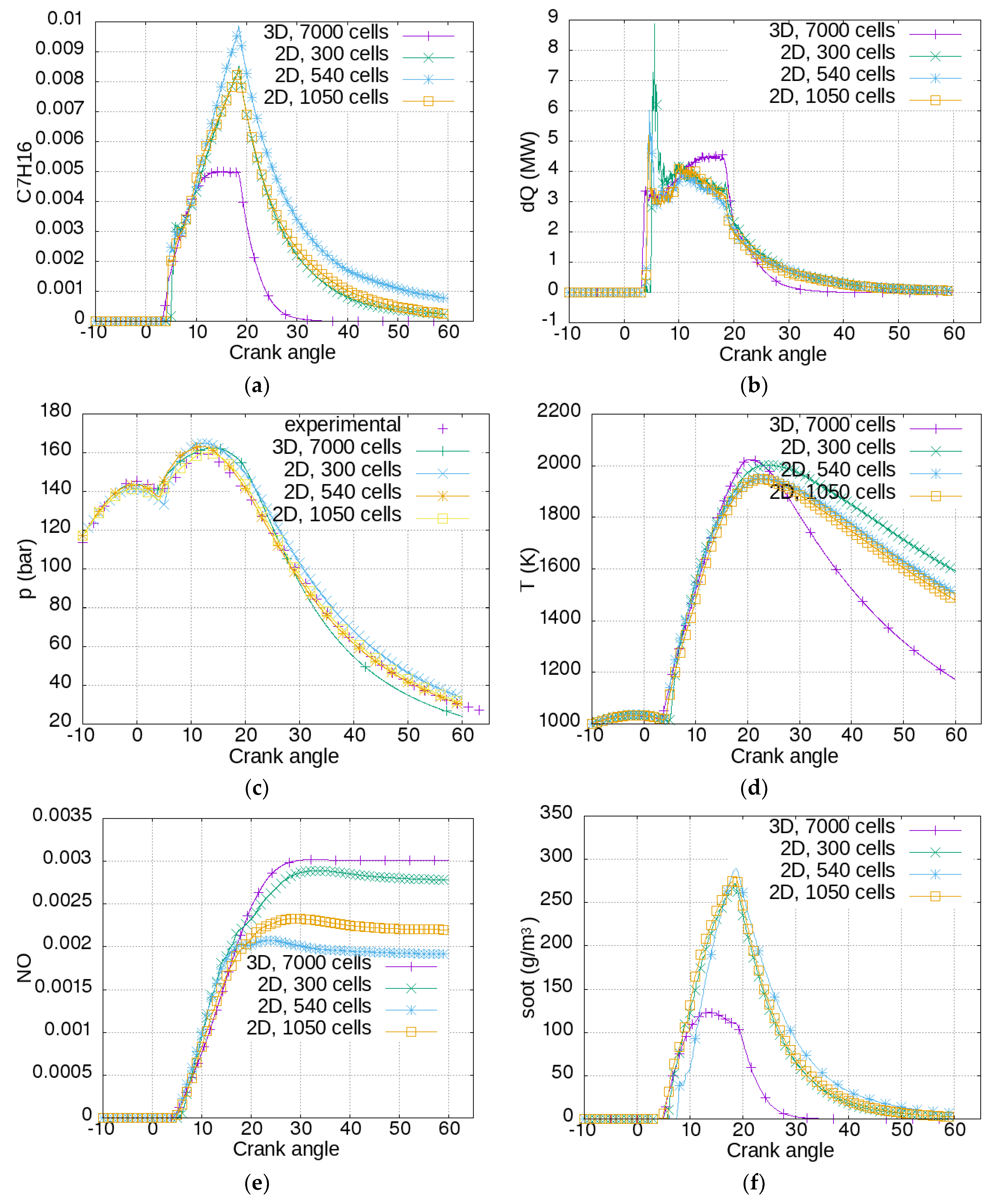
Figure 3.
The concentration of fuel vapor versus crank angle is shown in
Figure 3a. Injection starts at the TDC (top dead center—0 degrees). About 4 degrees are necessary for the beginning of the evaporation process. The increase of fuel vapor concentration is slowed down by the combustion process, which starts to consume fuel vapor. Evaporation and vapor consumption were in balance from 10 to 20 degrees for the 3D mesh, while for the 2D meshes the concentration peaked just before 20 degrees, after which the vapor was consumed rapidly, but some fuel remained unburnt until a crank angle of 60 degrees.
Figure 3b shows the rate of heat release. Combustion started slightly earlier for the 3D case, and hence the peak for premixed burning was higher for the coarser meshes. After the premixed burning, there was a gradual increase of the heat release rate for the 3D mesh until 18 degrees, after which combustion terminated around 30 degrees. For the 2D cases, combustion slowed down gradually until 45 degrees. In
Figure 3c, the cylinder pressure is presented for the simulation cases beside an experimentally obtained pressure function. Generally, all the simulations showed reasonable agreement with the experiment.
The coarsest mesh (2D, 300 cells) resulted in a higher ignition delay, which resulted in a slightly higher peak pressure. The most complex mesh (3D, 7000 cells) showed a higher pressure between 10 and 25 degrees, after which the pressure fell below the measured one. The 2D meshes of 540 and 1050 cells showed excellent agreement with the experimentally obtained values.
Figure 3d shows the main cylinder temperature for the different meshes. The 3D mesh reached the maximum of over 2000 K earlier, after which it fell rapidly. The temperature for the 2D meshes was very similar, but the temperature for the coarsest mesh was higher after a crank angle of 20 degrees. In
Figure 3e, NO concentrations for different meshes are presented. The characteristic trend was seen for all cases. NO production was intensive when combustion took place and when local temperatures exceeded 2000 K. The highest concentration was reached for the 3D mesh (0.003, or 3000 ppm), while it was lowest for the 2D, 540 mesh (about 0.002, or 2000 ppm). This can be recalculated to about 10 g/kWh, depending on the operation parameters.
IMO regulations define the maximum NOx emissions in g/kWh, while simulation and measurement results were obtained for NO concentration (ppm) in the exhaust gases. To obtain emission levels in g/kWh from ppm, the exhaust gas flow and the engine power also have to be measured. Power is measured on the test bench, but the exhaust gas flow is calculated from the engine speed, geometric dimensions, fuel consumption, scavenge air pressure, and temperature. These measurements are performed by engine factories, shipyards, and mostly environmental organizations. The results depend on fuel properties, environmental parameters, and measurement equipment. The engine factory solely guarantees that the engine fulfils certain limits (i.e., IMO Tier 1, 2, or 3). The engine studied in the article claims to fulfil IMO Tier 2 limits, which means an emission of NOx less than 14.4 g/kWh. Measurements on this engine [
30] yielded 12 g/kWh (average from three tests), which translates to 2300 ppm or an NO concentration of 0.0023 in the exhaust gases. The results obtained in the present paper were in the same concentration range (0.002–0.003). They were also comparable to the NO emissions obtained by other authors [
31].
Figure 3f shows the soot concentration. The lines show the typical trend of soot formation in the first part of the combustion, and intensive soot oxidation in the second part. The 3D mesh showed a lower amount of soot than the 2D meshes. For the 3D mesh, at the end of the simulated period the soot concentration amounted to 7.63 × 10
−13 g/m
3, while for the 2D meshes it amounted to 2.67 g/m
3, 6.35 g/m
3, and 2.28 g/m
3 for the meshes with 300, 540, and 1050 cells. The used model was very simple, and useful just to evaluate the sooting tendency of different setups. However, it manifested a typical trend over time. There was also a noticeable trade-off between soot and NO: the cases with highest NO emissions had the lowest soot emissions, and vice versa.
The cylinder pressure curves (
Figure 3c) showed very good agreement, regardless of the number of cells and domain dimensionality. On the other hand, the curves for fuel vapor (C7H16), rate of heat release (dQ), temperature (T), NO, and soot concentrations exhibited some variations between the 2D and 3D cases. The 2D cases were different from the 3D case in the number of cells, in the geometry of the heat exchange area, in the configuration of the injection nozzles, and in the characteristics of the reacting turbulent flow inside the cylinder. The 2D cases were a simplification of the 3D case, which is why the results of the 2D and 3D cases are different. Nevertheless, the differences were within acceptable limits, judging from the validation against experimental data of cylinder pressures and NO emissions. After the analysis of the calculation mesh influence, for the further analysis, the intermediate 2D mesh with 540 cells was selected. It gave very similar results to the 1050 cell mesh, the obtained cylinder pressure matched almost perfectly the experimental one, but the calculation took 58% less time compared to the 1050 cell mesh.
3.2. Water Injection
In the present section the most common water injection strategies are simulated and evaluated, namely intake air humidification, direct fuel–water emulsion injection, and direct water injection.
3.2.1. Intake Air Humidification
In this type of system, water droplets or vapor is introduced to the intake air, therefore generating a homogeneous distribution of water inside the engine cylinder [
5,
6]. The calculations were set by modifying the mass fraction of the mixture at the beginning of the calculation. Cases with 0% water, 10% water, and 20% water were performed. In
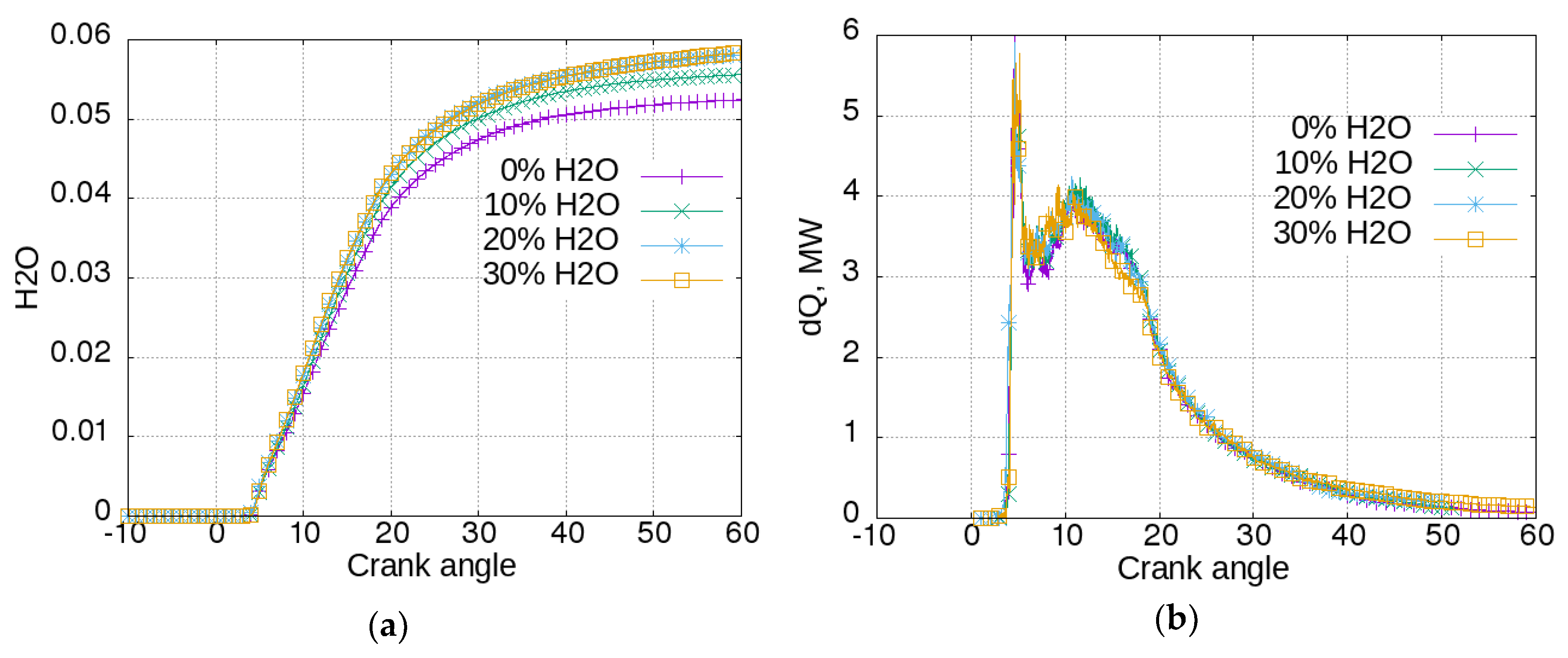
Figure 4, the influence of this strategy on engine operation is presented.
In
Figure 4a, the water concentrations for the three cases are shown. It can be seen that water concentration started to rise at a crank angle (CA) of about 4°. The reason for this is that water vapor is a combustion product. The concentration increased more for the case with an initial water concentration of 0, and less for the cases with greater initial concentration, since the produced H
2O has a greater relative impact. The heat release rate can be seen in
Figure 4b. Heat release is more intensive for the case without water added, and is proportionally reduced with the increase of initial water concentration. This reflects the cylinder pressure (
Figure 4c). It can be seen that humidified air reduced the pressure achieved in the cylinder, meaning that scavenge air humidification had a negative impact on engine power and efficiency. In
Figure 4d, the same trend was manifested by cylinder mean temperatures. The addition of 20% of water reduced the peak temperature by about 270 K. The temperature had a major influence on NO formation, which can be seen in
Figure 4e. The addition of 10% of water to the scavenge air could reduce the emission of NO by almost 50%. The influence of air humidification on soot emissions is shown in
Figure 4f. More intensive combustion in the case without water in the scavenging air promoted a more intensive soot production, as can be seen from the highest peak. However, it also promoted a more intensive oxidation. Hence, at the end of the calculated process, at CA = 60°, the concentration of soot was greater for the cases with higher water concentration—respectively 11, 10, and 6.5 g/m
3 for the cases with 20%, 10%, and 0% initial water content. Again, it can be said that, even if the soot model was very basic, it reproduced the opposite tendency of NO and soot formation.
3.2.2. Direct Fuel–Water Emulsion Injection
Another water introduction technique is direct fuel–water emulsion injection. This means that water is mixed with fuel before injecting it directly into the combustion chamber, via the same injector as fuel [
5,
6]. It does not allow water to be directed to a different location than the fuel, but it is technically simpler than injecting water via separate water injectors. The simulations were set by adding 10%, 20%, and 30% of water to the fuel injected, the amount of which was not altered. The influence of the water injection is presented in
Figure 5.
Figure 5a shows the cylinder water vapor concentration. Water concentration started to increase with combustion, 4 degrees after the start of injection. As expected, the increase was greater for the cases with water added to fuel, but the concentration of water vapor for the case with 30% water was not greater than that with 20% water. The explanation could be that there was not enough time or heat in the surrounding air to evaporate larger amounts of water.
Figure 5b presents the rate of heat release. The differences between the cases were small. It can be noticed that the rate was slightly smaller for the case with 30% water from 10 to 18 degrees of crank angle.
Figure 5c shows the cylinder pressure. There were no evident differences between the cases, except for the case with 30% water. This means that the direct addition of water to fuel did not have negative influence on engine efficiency or fuel consumption, at least for such small quantities of added water.
Figure 5d shows the cylinder temperature. The influence of the addition of 10% water to fuel was negligible. The addition of 30% water reduced the maximal mean cylinder temperature by about 100 K. Temperature reduction translates to a reduction in NOx formation, as can be seen in
Figure 5e. The increase of water percent in fuel resulted in a proportional NOx formation reduction. The case with 30% water in fuel allowed a reduction of NOx concentration from 0.00192 to 0.00164 or almost 15%.
Figure 5f shows soot concentration. It can be seen that water-in-fuel emulsion slightly increased soot formation, and inhibited soot oxidation. At the end of the simulated process, the soot concentration was several times higher for the cases with water in the fuel, especially for greater water concentrations. It is common that techniques that reduce NOx formation enhance soot formation.
3.2.3. Direct Water Injection
According to [
5,
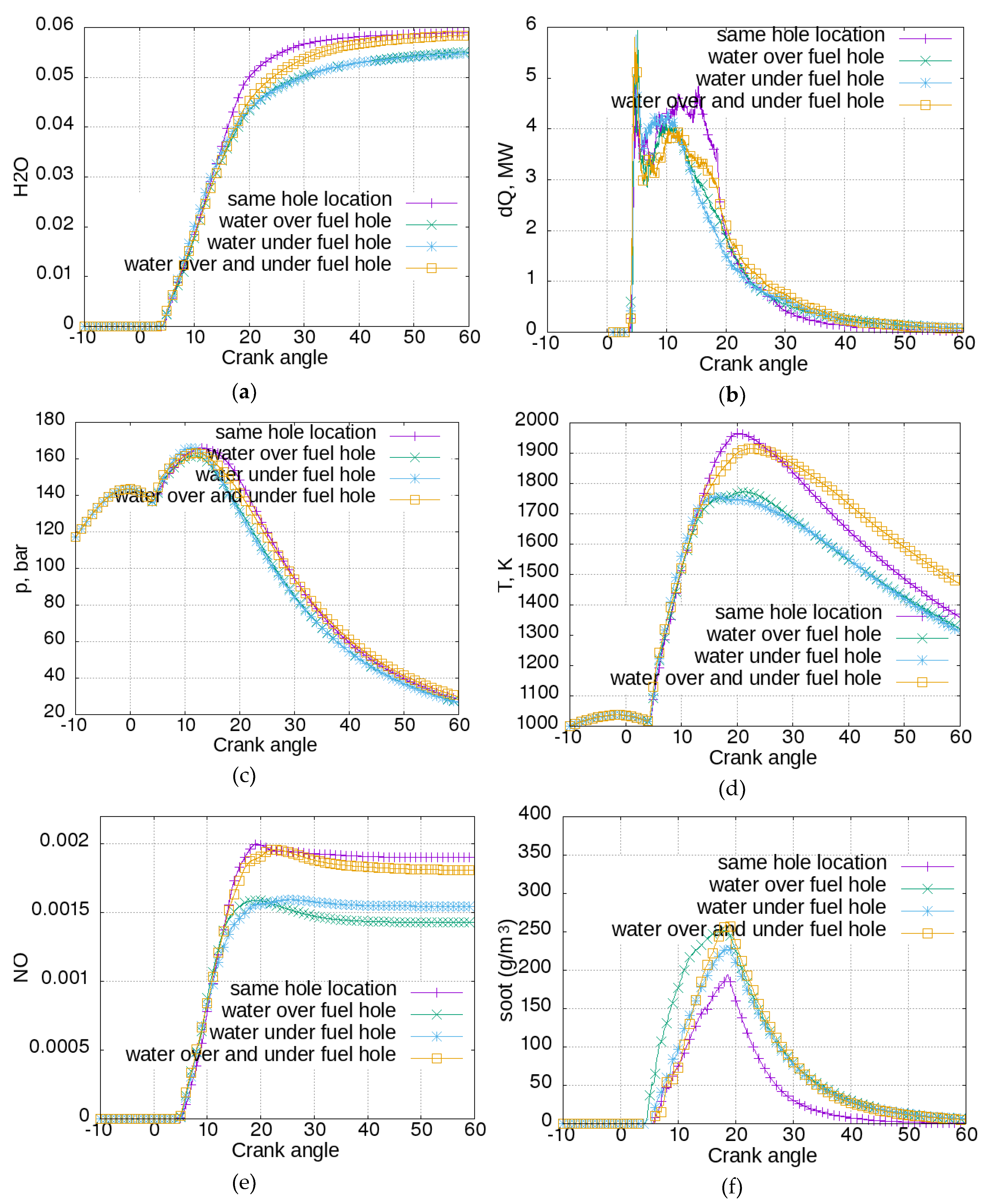
6], water is most efficient in NOx reduction when it is injected directly to the highest-temperature location, which is at the border of the fuel spray, where the fuel–air ratio is closest to stoichiometric, and where the combustion rate is highest. In order to achieve this, a separate injector for water has to be used, which complicates the cylinder construction. In this section, water injection from a separate injector was simulated. It was set to inject the amount of water corresponding to 20% of the injected fuel for all cases. In the first case, the location of the water injection coincided with the fuel injector. In the second case, the dedicated water injector was placed 2 cm over the fuel injector. In the third case, the dedicated water injector was placed 2 cm under the fuel injector. In the last case, two water injectors were placed 2 cm from the fuel injector—one above and the other under the fuel injector. In this case, the amount of water injected from each water injector was equal to 10% of injected fuel mass. The comparison of the described cases is reported in
Figure 6.
Figure 6a shows the water vapor concentration. The water concentration reached higher levels if it was injected from the same location as the fuel, or from two water injectors. If it was injected from a single water injector under or over the fuel injector, the attained water vapor concentration was lower.
Figure 6b shows the rate of heat release. The case with water injected from the same location as the fuel had a different behavior than the other cases. There was a lower initial heat rate peak from the premixed combustion and more intensive main diffusive combustion (from CA = 10 to CA = 18). The late burning after CA = 20 was more intensive for the cases with water injection from a separate location. The heat release rate was reflected by the cylinder pressure (
Figure 6c). There was an earlier pressure rise for the cases with water injection from a separate location. However, after the intensive diffusion combustion for the case with water injection from the same location, the pressure for this case was higher. The cylinder temperature is shown in
Figure 6d. Here the differences among cases were more evident: the temperatures for the cases with water injection from the same location as fuel and from two locations continued to rise after CA = 14, and reached 1964 and 1915 K, respectively. On the other hand, the cases with water injection from a hole above or under the fuel injection site reached lower maximal temperatures—respectively 1770 and 1756 K. Cylinder local temperatures had a key role in NO production, which is reported in
Figure 6e. The cases with higher temperatures resulted in higher NO concentrations. A different disposition of water injection allowed a 25% reduction of NO production to be achieved. In
Figure 6f, soot formation trends are presented for the different water injection configurations. Once again it can be seen that the case with greatest NO emissions resulted in the lowest soot levels.
Local temperatures were the main factor influencing thermal NO formation.
Figure 7 presents the temperature fields for the four simulated cases for the moment at CA = 15. Moving from left to right, there is the case with the same location of the water and fuel nozzle, the case with the water nozzle over the fuel nozzle, the case with the water nozzle under the fuel nozzle, and on the far right, the case with a water nozzle over and under the fuel nozzle. The fuel droplets are shown in red, while water droplets are shown in blue. The isolines for the constant water vapor concentrations of 0.7, 0.8, and 0.9 are also shown.
Figure 8 shows the NO concentrations for the same cases at the same moment. It can be concluded that water acts as a combustion damper, so temperatures were somewhat lower in the regions around the water spray. Finally, smaller regions with the highest temperatures resulted in lower NO concentrations. It was expected that the case with two water injectors would result in the lowest NO concentrations, which did not happen. However, a great deal of optimization could be done in terms of water spray direction, injected water quantity, nozzle size, and injection timing.
4. Conclusions
A 2D CFD approach is suggested in this article in order to calculate combustion and pollutant formation in large marine engines. This is especially important since such engine cylinders have large dimensions, and combustion chemistry tends to become very complex in order to simulate the latest emission reduction strategies. The OpenFOAM solver dieselEngineFoam was enhanced by adding heavy fuel oil data and by adding a basic soot model.
Three 2D simulation meshes were compared to a full 3D mesh simulation. Cylinder pressure was compared to the experimentally obtained pressure. The 2D simulations showed a very good agreement with the experimental results. The NO concentration showed a very realistic formation curve and absolute amount. The soot model also resulted in a realistic formation and oxidation trend. The soot simulation is useful for evaluating the influencing factors, since the absolute values can differ a lot from the measured ones. A 2D mesh with intermediate coarseness was selected for the further simulations.
It is concluded that 2D simulation offers a good compromise between QD and 3D simulations, and offers the capability of simulating engine emissions, as well as some geometric influences, such as the influence of nozzle location. It is also useful if many initial parameters has to be evaluated, since it is very fast compared to 3D calculations.
The value of the simulations was also confirmed in the second part, where water injection strategies were evaluated. Intake air humidification was modeled by modifying initial water concentration up to 20%. It showed that water vapor had a combustion damping effect. It reduced cylinder pressure and temperature. As a consequence, it was very effective in NO reduction, but it also reduced power and fuel efficiency. Direct fuel–water emulsion injection was simulated by adding up to 30% of water to the injected fuel. The simulation results showed that this method was efficient in reducing NO formation. The effect on pressure was negligible, hence it did not increase fuel consumption.
Finally, direct water injection via separate water injection nozzles was simulated. This method showed to have a great potential in reducing NO emissions because of its flexibility, but it has to be tuned and optimized carefully in order to inject water to the regions with highest local temperatures. However, it is the most complex to execute.
The simple Hyroyasu-inspired soot model showed a soot formation and oxidation trend known from the literature. It also showed a typical behavior when methods that reduced NOx formation tended to result in increased soot emissions. However, there was no intention to simulate the exact amount of soot at the end of the process, and hence no parameter optimization was performed. A more precise and sensitive soot model should be developed, but it was beyond the scope of this article.
NO concentration was simulated more accurately. Even if precise measurements for the engine are not available, the limits prescribed by the International Maritime Organization are in g/kWh. If the cylinder concentration is calculated to g/kWh, some calculations reached about 10–15 g/kWh, which could satisfy IMO Tier 2. In order to get better results in terms of NO reduction without penalties to fuel efficiency or soot formation, a more detailed simulation set would be required. Water injection parameters such as nozzle direction, size, injected water quantity, flow, temperature, and injection timing should be optimized. For the detailed nozzle orientation tuning, a 3D model would be necessary.


