Joint Inversion for Sound Speed Field and Moving Source Localization in Shallow Water

Abstract

This paper develops a joint approach for time-evolving sound speed field (SSF) inversion and moving source localization in shallow water environment. The SSF is parameterized in terms of the first three empirical orthogonal function (EOF) coefficients. The approach treats both first three EOF coefficients and source parameters (e.g., source depth, range and speed) as state vectors of evolving with time, and a measurement vector that incorporates acoustic information via a vertical line array (VLA), and then the inversion problem is formulated in a state-space model. The processors of the extended Kalman filter (EKF) and ensemble Kalman filter (EnKF) are used to estimate the evolution of those six parameters. Simulation results verify the proposed approach, which enable it to invert the SSF and locate the moving source simultaneously. The root-mean-square-error (RMSE) is employed to evaluate the effectiveness of this proposed approach. The interfile comparison shows that the EnKF outperform the EKF. For the EnKF, the robustness of the approach under the sparse vertical array configuration is verified. Moreover, the impact of the source-VLA deployment on the estimation is also concerned.

1. Introduction

Ocean parameter inversion and source localization are practical problems with serious concerned and long standing applications in underwater acoustics [1,2]. A common feature of these problems is that underlying environment parameters are estimated from measured acoustic data. The sound speed profile (SSP), one of the important environment parameters extracts from ocean properties, has a significant influence on determining acoustic waveguide propagation [3]. Oceanographic variability and dynamic processes cause the SSP evolve in time and space, especially in shallow water areas [4,5]. The SSP can be obtained by combining model outputs or in situ measurement, however, the temporal and spatial sampling from a large area within a short time and long-term observation is often unrealistic. Numerous approaches have been developed to invert the sound speed in the water volume fast and accurate. To reduce the degrees of freedom, ocean parameters include the SSP are often represented in terms of EOFs [6,7]. The previous studies indicate that the inversion of SSP has a good agreement with the measured data, in both shallow [8] and deep ocean [9]. Besides, the compressive estimation of SSP using EOFs is demonstrated in reference [10]. These characteristics of the spatiotemporal variability can be transformed to an estimating problem.

Since the introduction of the Kalman filter (KF) [11], much more researches on KF family and their extensions have been implemented for practical issues. These filters are suitable approaches to estimate the nonlinear and non-Gaussian problems, and have been used previously in underwater acoustic application [12,13,14]. An excellent overview described that sequential filtering provide a suitable framework for estimating and updating the parameters of a system as data become available, examples include target localization, spatial arrival time tracking and geoacoustic inversion [15]. Yardim et al. formulated the evolution of environmental parameters by extended Kalman filter (EKF), unscented Kalman filter (UKF) and particle filter (PF), which converted geoacoustic inversion into tracking techniques [16]. Carrière put forward a state-space model for acoustic measurement data assimilation problem, and inverted the SSF by EnKF firstly [17]. Reference [18] proposed an improved algorithm compared with the performance of PF and EnKF to track the SSP, the improved filter had a better accuracy but computational complexity was greatly increased. However, the above methods have not considered source state, and it employed a traditional fixed source–receiver system, which has a lower spatial resolution. The geoacoustic characterizations of wide areas through inversion require easily deployable configurations including free-drifting platforms, underwater gliders and autonomous vehicles [19]. By employing a moving source launch signal to get high resolution, the information of the acoustic field is increasing. Afterwards, Dosso et al. examined the motion-compensated acoustic localization, which performed much better than static-model localization method or a localization based on applying fixed travel-time corrections [20]. In addition, based on the theory of compressed sensing, several algorithms are applied to direction-of-arrival (DOA) tracking, Das formulated the tracking problem of recovering a low-rank matrix and a sparse matrix by considering all snapshots together, rather than estimating the DOA snapshot-by-snapshot [21]. Guiding by the above-mentioned, our motivation and interest in this paper is proposing a joint scheme to reconstruct the SSF and locate the source simultaneously, rather than carrying out in separate inversion steps.

To perform the inversion, source parameters (such as source location) should be taken into consideration. Meanwhile, from the time-evolving information we can derive parameters such as depth and range of the source inversely. In the present study, nonlinear filters of EKF and EnKF are used as the processor, which are analyzed and calculated by numerical simulations. The estimating capabilities of the processors are compared with synthetic acoustic pressure data and the measured data collected during the ASIAEX (Asian Seas International Acoustics Experiment) ECS (East China Sea) 2001 experiment.

The remainder of the paper is organized as follows: The theory of SSF parameterization and the state-space model is introduced in Section 2. Section 3 covers the essential algorithms of EKF and EnKF. Simulation results of the proposed approach are discussed and compared in Section 4. For the EnKF, a robustness inversion scheme under the sparse vertical array configuration and impact of the source-vertical line array (VLA) deployment on the estimation are given. Finally, Section 5 concludes the paper.

2. A State-Space Model for Joint Inversion

In this work, the inversion of SSF is carried out in the unit of SSP. An independent SSP can be measured in each time interval. Combining these discrete adjacent intervals, the approximate distributions of sound speed variation in continuous time are obtained. In this section, theory of SSF parameterization is summarized briefly, and then the mathematical model of the moving source tracking is given.

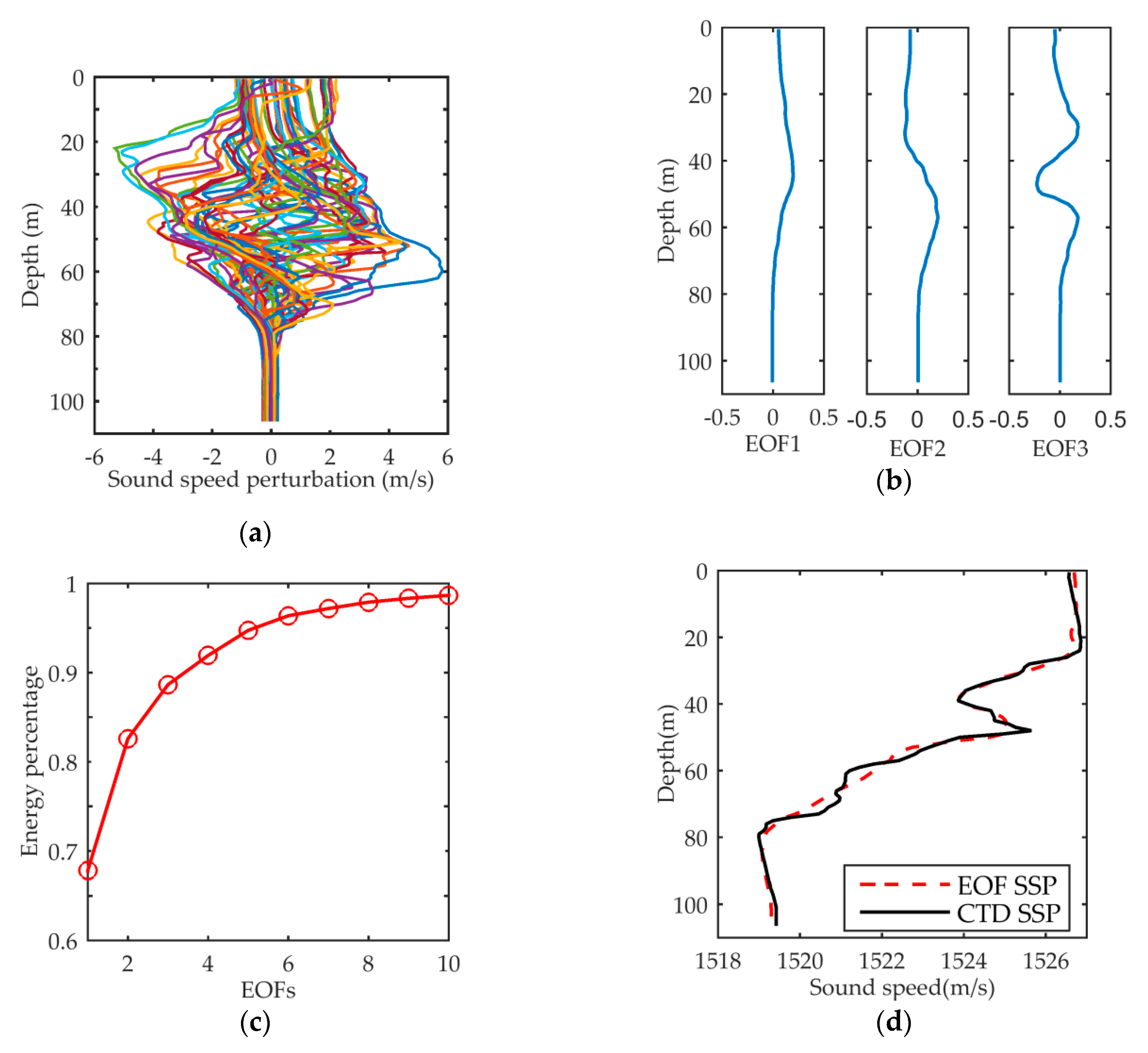
2.1. Sound Speed Field Parameterization

EOF is a reasonable way to fully parameterize the SSP [22], which can be obtained from a direct measurement of database and are efficient in reducing the degrees of freedom of estimated parameter vector.

Assuming that there are $N$ SSP measurements $c_1\left(z_i\right),c_2\left(z_i\right),\cdots c_N\left(z_i\right)i=1,2,\cdots ,M$, where $M$ is the number of discrete points in depth. The mean sound speed is given by $\overline{c}(z)=\frac{1}{N}{\displaystyle \sum _{i=1}^N{c}_i\left(z\right)}$, and the sound speed perturbation is expressed as:

$$\mathsf{\Delta }{c}_i\left(z_j\right)=c_i\left(z_j\right)-\overline{c}\left(z_j\right),$$

(1)

where $c_i\left(z_j\right)$ denotes the sound speed value at depth $j$ of the $i$-th SSP. The sample covariance matrix $R$ is computed to characterize the uncertainty of the sound speed:

$$R=\frac{1}{N}\left[\begin{array}{cccc}\mathsf{\Delta }{c}_1\left(z_1\right)& \mathsf{\Delta }{c}_2\left(z_1\right)& \cdots & \mathsf{\Delta }{c}_N\left(z_1\right)\\ \mathsf{\Delta }{c}_1\left(z_2\right)& \mathsf{\Delta }{c}_2\left(z_2\right)& \cdots & \mathsf{\Delta }{c}_N\left(z_2\right)\\ ⋮& ⋮& ⋮& ⋮\\ \mathsf{\Delta }{c}_1\left(z_M\right)& \mathsf{\Delta }{c}_2\left(z_M\right)& \cdots & \mathsf{\Delta }{c}_N\left(z_M\right)\end{array}\right]{\left[\begin{array}{cccc}\mathsf{\Delta }{c}_1\left(z_1\right)& \mathsf{\Delta }{c}_2\left(z_1\right)& \cdots & \mathsf{\Delta }{c}_N\left(z_1\right)\\ \mathsf{\Delta }{c}_1\left(z_2\right)& \mathsf{\Delta }{c}_2\left(z_2\right)& \cdots & \mathsf{\Delta }{c}_N\left(z_2\right)\\ ⋮& ⋮& ⋮& ⋮\\ \mathsf{\Delta }{c}_1\left(z_M\right)& \mathsf{\Delta }{c}_2\left(z_M\right)& \cdots & \mathsf{\Delta }{c}_N\left(z_M\right)\end{array}\right]}^T$$

(2)

where T is the transpose. Using the orthogonal decomposition, we have $R={\displaystyle \sum _{n=1}^M{\lambda }_n{f}_n{f}_n^T}$, where ${\lambda }_1>{\lambda }_2>\cdots >{\lambda }_M$ are the respective eigenvalues of eigenvectors $f_n$. Due to the eigenvalues diminishing rapidly, only a few EOFs are able to dominate the SSP characterization. Therefore, each SSP in the ocean can be approximated with the first K eigenvectors as:

$$c\left(z\right)=\overline{c}\left(z\right)+{\displaystyle \sum _{k=1}^K{\alpha }_k}{f}_k\left(z\right),$$

(3)

where ${\alpha }_k$ and $f_k\left(z\right)$ are called the $k$th EOF coefficient and EOF, respectively.

As stated above, inversion for SSF is a multi-dimensional optimization problem. The computational complexity and inversion accuracy usually depend on the number of inverted variables. Therefore, a limited number of EOFs are used to invert the SSF. Assuming the number of EOFs to be retained $K$ is based on the amount of total energy contained in the associated eigenvalues $\{{\lambda }_i\}$. Defining the ratio of partial-total energy as a percentage:

$$\rho \left(K\right)=\frac{{\sum }_{i=1}^K{\lambda }_i}{{\sum }_{i^{\prime }=1}^N{\lambda }_{i^{\prime }}}100,\rho \left(K\right)|{I=N}_{}=100\%,$$

(4)

where $N$ is the total number of eigenvalues, which enable us to select $K$.

In order to demonstrate the effectiveness of inversion method, data measured in the 2001 ASIAEX, ECS experiment were used [23]. The sound speeds were obtained from the onsite conductivity–temperature–depth (CTD) measurements. They were sampled at 106 discrete depth points from the surface to the bottom, equally spaced by 1 m.

Figure 1a shows 54 samples of sound speed perturbations, which were calculated by the SSP data measurements, the fluctuation amplitude was more than 11 m/s between 20 m and 60 m in depth. The variability of SSP was modeled using EOF by calculating from Equations (2) and (4), and the first three EOFs are plotted in Figure 1b. In this case, Figure 1c shows that choosing $K=3$ could represent approximately 90% of the energy disturbance. Then, the first three EOFs were chosen to invert the $p$th SSP in 54 measured samples, the EOF coefficient was calculated as ${\alpha }_k={\left[c_p\left(z\right)-\overline{c}\left(z\right)\right]}^T{f}_k\left(z\right),k=1,2,3$, it is seen that the inverted SSP was in good agreement with the measured SSP in Figure 1d. The depth-integrated RMSE was employed to evaluate the discrepancy between the measured SSP and inverted SSP. After calculation, the RMSE of inverted SSP by EOF was 0.37 m/s. As the result, the first three EOFs were capable of represent SSP.

As introduced above, the inversion problem of SSP corresponds to the projection of first three EOF coefficients. The proposed scheme developed in the paper was to reconstruct the time-evolving SSF. The SSF evolution of vertical slice was then discretized into a finite number of adjacent rectangular intervals, each of which describes its characteristics with an independent SSP. Dividing the evolution into $L$ intervals and using the first three EOFs. For the $l$th interval, the sound speed was calculated in the form of:

$$c\left(R_{l-1,z}<l\le R_{l,z}\right)=\overline{c}\left(z\right)+{\displaystyle \sum _{k=1}^3{\alpha }_{k,l}{f}_k\left(z\right)},$$

(5)

where ${\alpha }_{k,l}$ is the $k$th EOF coefficient of the $l$th profile. In this way, any sound speed estimates should be constrained to lie in the evolution of the EOFs. That is, the SSF is recovered by a total of $l$ SSPs, and the coefficients ${\alpha }_{k,l}$ constitute the SSF parameters.

2.2. The Mathematical Model of the Joint Inversion

The joint inversion for SSF and source localization requires two dynamic equations: A state equation that models the evolution of SSF and the movement of source, and a measurement equation that relates the environment and source location at step $k$ to the acoustic field.

It is known that ocean sound speed can be parameterized in terms of the first three EOF coefficients in Section 2.1. In this work, we have:

$${\mathsf{\alpha }}_{k|k-1}={\left[\begin{array}{c}{\alpha }_1\\ {\alpha }_2\\ {\alpha }_3\end{array}\right]}_k=\left[\begin{array}{ccc}1& 0& 0\\ 0& 1& 0\\ 0& 0& 1\end{array}\right]{\left[\begin{array}{c}{\alpha }_1\\ {\alpha }_2\\ {\alpha }_3\end{array}\right]}_{k-1}+w_k.$$

(6)

$w_k$ is the state noise vector. For a moving source, the depth $Z$, horizontal range $R$, and radial speed $v$ are to be estimated:

$$s_{k|k-1}=\left[\begin{array}{c}{Z}_{k|k-1}\\ R_{k|k-1}\\ v_{k|k-1}\end{array}\right]=\left[\begin{array}{ccc}1& 0& 0\\ 0& 1& \mathsf{\Delta }t\\ 0& 0& 1\end{array}\right]\left[\begin{array}{c}{Z}_{k-1|k-1}\\ R_{k-1|k-1}\\ v_{k-1|k-1}\end{array}\right]+\left[\begin{array}{cc}1& 0\\ 0& \mathsf{\Delta }{t}^2/2\\ 0& \mathsf{\Delta }t\end{array}\right]\left[\begin{array}{c}{v}_d\\ v_a\end{array}\right]k=1,\cdots K,$$

(7)

where $s$ denotes the source parameters, $\mathsf{\Delta }t$ is the update time increment (i.e., the time interval between two measurements), and $v_d$ and $v_a$ are the random variables representing the variation in source depth and acceleration, respectively.

Then the state vector that includes the parameters of source and SSF is given by merging these two blocks. Defining the state vector as $x_k^T=\left[s_k^T{\mathsf{\alpha }}_k^T\right]$. The state and measurement equations are considered as:

$$x_k=f(x_{k-1})+v_{k-1},$$

(8)

$$y_k=h(x_k)+w_k,$$

(9)

where $f(\cdot )$ is a state transition function of the state vector $x_{k-1}$, and $h(\cdot )$ is the normal mode propagation model, and $v_k$ and $w_k$ are the process/state and measurement noise vectors, respectively. Here, $y_k$ is the acoustic pressure measured at $k$th time frame, the measurement equation was used to characterize the signal of acoustic pressure, which was received by a VLA. According to the normal mode theory, the synthetic acoustic pressure can be expressed as a general nonlinear function of the horizontal range $R$, depth $Z$ and sound speed $c$.

As mentioned above, the state equation describes the evolution of the SSF and source location, and the measurement equation relates the state vectors and ocean environment to the acoustic field. In this way, the state-space model is used as a sequential method enable to estimate the evolving state.

3. Nonlinear Kalman Filter as an Inversion Processor

In dynamical evolution of time-evolving SSF and moving source localization, the processor of the sequential method is used to predict and estimate the joint inversion results. For the nonlinearity of measurement function $h(\cdot )$, two kinds of nonlinear filtering algorithms are given as follows.

3.1. EKF Model

A common Kalman filter applied to the nonlinear systems was EKF. Since KF is an exact linear tracking filter, its extended version works by converting the system into a form over which the KF can operate. In an EKF, this is done by locally linearizing the state and measurement equations using the first order Taylor series expansion of the nonlinear transformations (such as the normal mode propagation model $h(\cdot )$). After linearization, the state and measurement equations given in (17) and (18) to:

$$x_k\approx f\left(\widehat{x}\left(k-1\right)\right)+F_k\left(x\left(k-1\right)-\widehat{x}\left(k-1\right)\right)+v_{k-1},$$

(10)

$$y_k\approx {\widehat{y}}_k+H_k\left(x_k-{\widehat{x}}_k\right)+w_k,$$

(11)

where $F_k$ and $H_k$ are Jacobian matrices of $f$ and $h$, respectively.

Table 1. Kalman Filter.

Principles
Predict: ${\widehat{x}}_{k|k-1}=f\left({\widehat{x}}_{k-1|k-1}\right)$ $P_{k|k-1}=F_k{P}_{k-1|k-1}{F}_k{}^T+W_k$
Update: ${\widehat{x}}_{k|k}={\widehat{x}}_{k|k-1}+K_k\left(y_k-h_k\left({\widehat{x}}_{k|k-1}\right)\right)$ $P_{k|}{}_k=\left(I-K_k{H}_k\right)P_{k|}{}_{k-1}$
Kalman gain: $K_k=P_{k|}{}_{k-1}{\widehat{H}}_k{}^T{\left(H_k{P}_{k|}{}_{k-1}{H}_k{}^T+V_k\right)}^{-1}$
Jacobians: $F_k=\frac{\partial f_k}{\partial x_{k-1}}{|}_{x_{k-1}={\widehat{x}}_{k-1|k-1}}$ $H_k=\frac{\partial h_k}{\partial y_k}{|}_{x_k={\widehat{x}}_{k|k-1}}$

summarizes the principle of EKF, applied to the proposed state-space model. In order for EKF to perform well, nonlinearities should be small and the underlying densities should also be close to Gaussian.

3.2. EnKF Model

The EnKF is a KF that includes Monte Carlo sampling, which enables us to deal with moderate nonlinear and non-Gaussian problems. The basic principle is initializing a set of system state samples as a background ensemble, and then using the latest observation information to update each background ensemble member in current time by Kalman filter to obtain the analysis ensemble. The sampling ensemble is transferred by the system model to get the background ensemble of the next time. Each member is propagated through the state transition and measurement functions and the statistics of the estimates are propagated without the use of any linearization step. An EnKF algorithm is summarized in

Table 2. Ensemble Kalman Filter.

Principles
Definitions
$X_k=\left\{x_{k,i},i=1,2,\cdots ,N\right\}$ Background ensemble member: Where $i$ is the ensemble member index and $k$ is the time frame
${\overline{x}}_k$ Background ensemble mean value at $k$
$X_k^a=\left\{x_{k,i}{}^a,i=1,2,\cdots ,N\right\}$ Analysis ensemble member
${\overline{x}}_k^a$ Analysis ensemble mean value at $k$
$z_{k,i}=y_k+{\epsilon }_i$ Ensemble of observation
$R_k=\frac{1}{N-1}{\displaystyle \sum _{i=1}^N{\epsilon }_i}{\epsilon }_i^T$ Ensemble covariance matrix
Predict:
$x_k=x_{k-1}^a+w_k$
$P_{xh}^k=\frac{1}{N-1}{\displaystyle \sum _{i=1}^N\left(x_{k,i}-{\overline{x}}_k\right)}{\left(h(x_{k,i})-h({\overline{x}}_k)\right)}^T$
$P_{hh}^k=\frac{1}{N-1}{\displaystyle \sum _{i=1}^N\left(h(x_{k,i})-h({\overline{x}}_k)\right)}{\left(h(x_{k,i})-h({\overline{x}}_k)\right)}^T$
Update:
$x_{k,i}^a=x_{k,i}+G_k\left(z_{k,i}-h\left(x_{k,i}\right)\right)$
$P_k^a=\frac{1}{N-1}{\displaystyle \sum _{i=1}^N\left(x_{{}_{k,i}}^a-{\overline{x}}^a{}_k\right)}{\left(x_{{}_{k,i}}^a-{\overline{x}}^a{}_k\right)}^T$
Kalman gain:
$G_k=P_{xh}^k{\left(P_{hh}^k+R_k\right)}^{-1}$

.

4. Results and Discussion

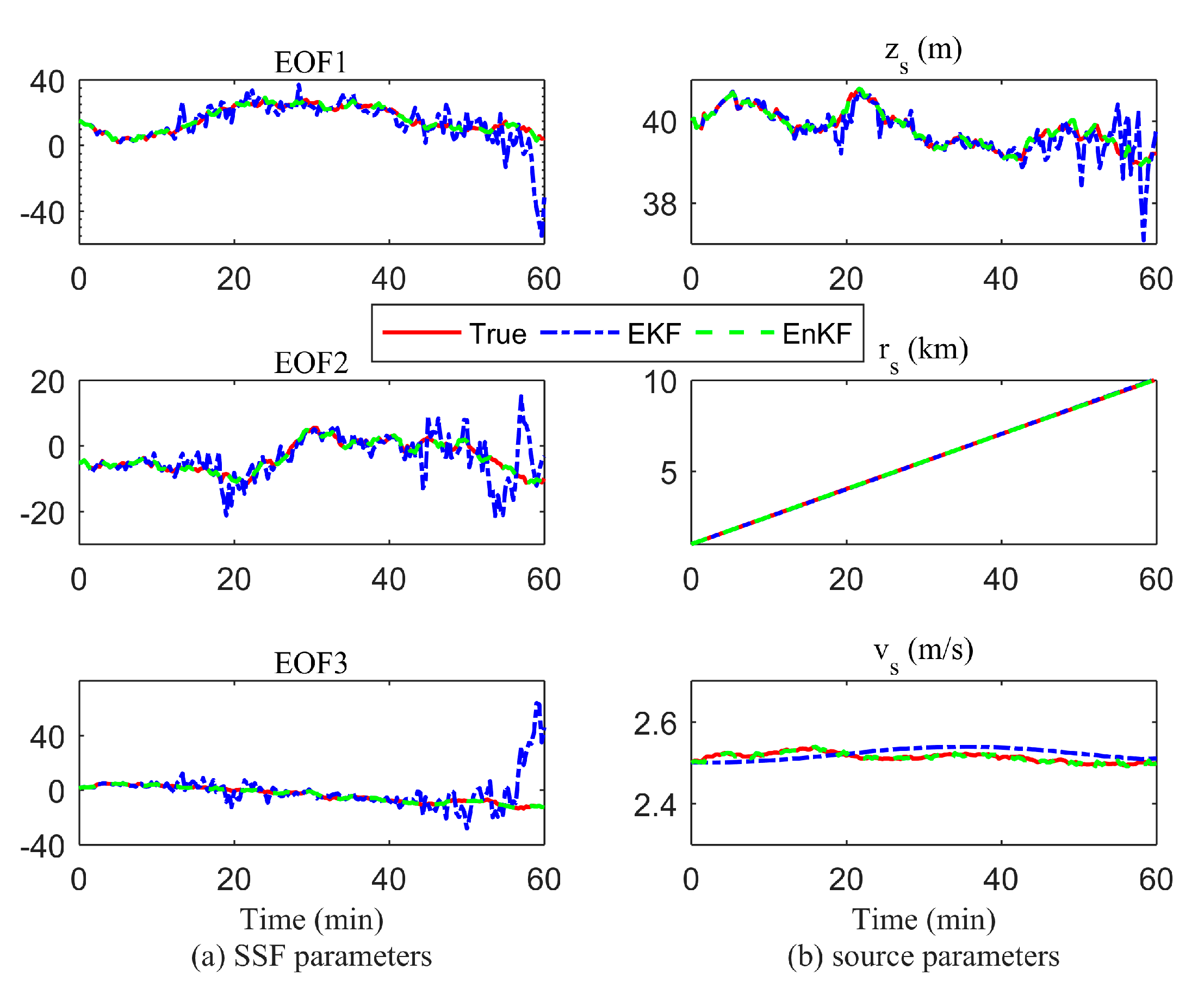
4.1. Estimation of EKF and EnKF for SSF and Moving Source Localization

To synthesize the acoustic pressure data used in the measurement equation, the simulated environment is shown in Figure 2. The water depth was 106 m according to the measurement. The bottom was modeled as a homogeneous fluid half space, which consisted of the silt clay sediment (sound speed of 1610 m/s, density of 1.7 g/cm³, and attenuation rate of 0.1dB/λ). These values of the geoacoustic parameters correspond to average values deduced from the core measurements of AXIAEX, ECS, 2001 [23]. The VLA was configured with 16-element equispaced 4 m that spanned the 15–75 m water depths. The source was placed at 40 m in depth and 1 km in range with a frequency of 400 Hz. Moreover, the source had 180 steps ($k=1,\cdots ,180$) movements away from VLA with the speed of 2.5 m/s. As a result, the continuous SSF was discretized in 180 intervals with the corresponding SSPs.

For the EnKF, the ensemble number is related to the precision and computational complexity. In order to balance the trade-off between the computational complexity and estimation accuracy, the ensemble number was set to $N=50$. We assumed that both additive noise terms $v_k$ (in Equation (8)) and $w_k$ (in Equation (9)) were represented by the Gaussian probability density functions. The adiabatic normal mode propagation model was used to compute the acoustic field by inputting the environmental and source parameters (except source speed) into KRAKENC [24]. As the state-space model described in Section 2.2, the first three EOFs coefficients and source parameters (depth, range, speed) were taken as the state vectors, and the acoustic pressures received by VLA were served as the measurement vectors. Under the proposed joint approach, the evolutions of EOFs coefficients were estimated to reconstruct the SSF, and the source parameters were tracking over time to give the localization. That is, this approach needs to estimate the evolution of those six parameters simultaneously.

The evolution of the six parameters is presented in Figure 3, where the estimation results were compared with the true values. We found that two filters were able to estimate the parameters. For the EKF, the processor shows good tracking performance at the beginning. However, there were divergences between the estimation results and true trajectories over time. It was seen from the curves of the first three EOFs coefficients in Figure 3a and source depth in Figure 3b, the large divergences appeared around the 55–60th min. As it describes, we found that the estimation of source depth would be affected when the EOF coefficients were not tracked well. The one reason for this phenomenon was explained that the acoustic pressure field was more sensitive to the depth of the source in normal mode theory. The other one was related to the basic assumption of the random walk in the state-space model. Noting that there were rapid perturbations of sound speed in some regions of the true environment, the above assumption might be explained that the perturbations result in larger variations of the EOF coefficients, which exceed the statistical values assumed for the random walk, thus resulting in a model mismatch. In addition, Figure 3a shows tracking of the EOF3 was worse than EOF1 and EOF2 coefficients. The possible reason was attributed to the third EOF playing a minor position compared with the first two orders on dominating the SSP perturbation, which leads to a minor variation of the sound speed in Equation (3). In the measurement equation, a little pressure variation information will affect the processor to track. By comparison, the estimation results confirmed that the EnKF was superior to the EKF. The EnKF was capable of estimating all parameters with a stable and narrower fluctuant result, which almost coincided with the true value completely.

According to the above estimation results of EOF coefficients, both two filters enabled us to reconstruct the true SSF, the inversion of SSF is shown in Figure 4. Figure 4b,d show pseudo-color maps of the relative error between estimated SSF and true SSF. Moreover, the errors near the thermocline were larger than the other regions. The inverted SSF of an EKF as Figure 4a,b indicates that the processor was correctly tuned at the beginning of estimation, but the sound speed mismatched because of the disturbance appeared around the 55–60th min, that was corresponding with the evolution of EOFs coefficients in Figure 3a. From Figure 4c,d, the EnKF shows a steady estimated result, especially in the region where intensive perturbation of sound speed existed. Meanwhile, the relative errors stay near-zero over the whole evolution period.

For both two filters, the inversion performance of SSF and source parameters was evaluated by root-mean-square-errors (RMSE) between the true values and estimated results. The RMSE curves of SSF and source parameters were calculated as shown in Figure 5, for comparison. We found that both processors still converged during an hour, but the RMSE values of EKF were much larger than EnKF. The values of SSF were especially enlarged (the maximum RMSE value was close to 7 m/s for the EKF) around the 55–60th min, which could be predicted by the tracking results in Figure 4. After calculation, the time-average RMSE values of SSF, source depth, range and speed for EKF were 0.6675 m/s, 0.0134 m/s, 0.8736 m/s and 0.0013 m/s, respectively. The EnKF, in contrast, maintained a low stable value of RMSE, which time-average values remained near-zero clearly. Therefore, it could be concluded that the EnKF outperformed EKF of this joint approach.

The main reason for this different estimated capacity of two filters can be summarized as follows: In an EKF, the covariance matrices propagated through the nonlinear model with the Jacobian of the transition and measurement functions. Such a first-order approximation, which ignores the higher-order terms, could result in large estimation errors, which could cause the filter to diverge (the gain tends to zero). In the inversion scheme, high nonlinearity of the measurement function requires high-dimensional nonlinear methods. While, the EnKF represents the underlying distributions with a large ensemble of model realizations, and the statistics of estimates are propagated without the use of any linearization step. It is a method for nonlinear transformation of the mean value and covariance to be practical for the realistic high-dimensional system [25].

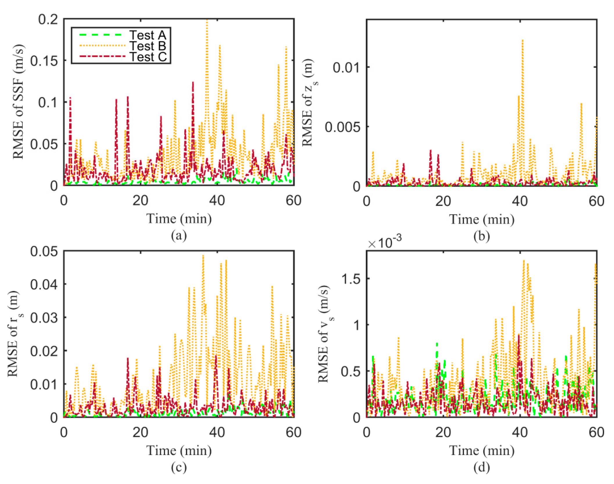
4.2. Sparse Array Configuration

In the above simulation, the initial configuration was a 16-element VLA. However, it is of practical interest to study whether the joint approach was robust when using a few hydrophones or a shorter array. The EnKF of better performance was chosen as a processor. The different configurations tested are given in

Table 3. Simulated array configurations with different hydrophones and spacing.

Test No.	#Hydrophones	Depths
A	16	15–75 m, 4 m spacing
B	8	15–75 m, 8.57 m spacing
C	8	30–58 m, 4 m spacing

. Keeping the other parameters settings consistent with the Figure 2, and reducing the number of VLA to 8-element in Test B (few hydrophones) and C (shorter array) to compare with Test A.

The evolutions of six parameters within an hour were estimated for three different tests, and the inversion for SSF under sparse array configuration is shown in Figure 6. The existence of fast-changing sound speed near the thermocline made a larger disturbance for EOF coefficients, which led to increased error. The inversion performances are summarized by the time-evolving RMSE in Figure 7. Although the estimation of EnKF was always converged, the RMSEs of Test B were larger than the other tests, seen from the curves of both SSF and source parameters. Moreover, we found the values of RMSE were enlarged around 40 and 55th min, that was due to the EOF coefficients (i.e., SSP) that were impacted with sound speed perturbation, especially in Test B and C.

Table 4. Time-average RMSE of EnKF for different test in Table 3.

Test No.	SSF	${\mathit{z}}_{\mathit{s}}$	${\mathit{r}}_{\mathit{s}}$	${\mathit{v}}_{\mathit{s}}$
	(m/s)	(10−4m)	(m)	(10−4m/s)
A	0.0045	1.0731	0.0013	1.7084
B	0.0354	9.7445	0.0109	3.9471
C	0.0186	2.9726	0.0031	1.8864

gives the time-averaged RMSEs of the three tests. As expected, the joint inversion performance mainly depended on the number of effective measurements. For a same given number of measurements, the approach was more suitable for the case involving a smaller spacing in depth (see Test B versus C). Test B gave the least accurate estimation, while Test A, characterized by the maximum number of measurements, outperformed the other configurations. Compared with 16-VLA, the RMSEs of the 8-VLA in the same time dimension increased slightly. Such differences might be explained that both the sparse elements and large spacing reduced the rate of spatial sampling, which led to an increasing error. To sum up, EnKF was a superior processor to invert the SSF and locate the moving source. Simulation results show the approach was robust even under a short array or lack of hydrophone elements.

4.3. Impact of the Source-VLA Deployment

With the gradual development of underwater vehicles in practical applications, the position of the source will be more flexible. As it is known from the normal mode theory, the source in different depths excites relative modes to represent the acoustic field, which may have an impact on the performance of the joint approach. The influence of the source–receiver deployment on the estimation is necessary to concern. To evaluate the effective of the joint approach, the source was placed at 10/96 m in depth, and moved away from the VLA in a horizontal direction. The VLA with 16 and 8 elements were deployed spanning upper/middle/bottom part of the water, respectively. After simulation, the time-average RMSEs of EnKF for SSF, source depth, range and speed estimation are listed in

Table 5. Time-average RMSE of EnKF for the source-vertical line array (VLA) deployment configurations.

		16-VLA					8-VLA
Source Depths	VLA Depths	SSF	${\mathit{z}}_{\mathit{s}}$	${\mathit{r}}_{\mathit{s}}$	${\mathit{v}}_{\mathit{s}}$	VLA Depths	SSF	${\mathit{z}}_{\mathit{s}}$	${\mathit{r}}_{\mathit{s}}$	${\mathit{v}}_{\mathit{s}}$
(m)	(m)	(m/s)	(10−4m)	(m)	(10−4m/s)	(m)	(m/s)	(10−4m)	(m)	(10−4m/s)
10	1–61	0.0108	4.9886	0.0012	3.1329	17–45	0.0454	5.8863	0.0060	2.5132
	23–83	0.0022	0.4614	0.0005	1.3260	39–67	0.0130	3.4522	0.0023	1.5162
	45–105	0.0030	1.3979	0.0006	1.3952	61–89	0.0257	4.0057	0.0025	1.6202
96	1–61	0.0041	2.6118	0.0007	1.5324	17–45	0.0232	5.1153	0.0049	2.1093
	23–83	0.0028	1.8307	0.0007	1.5090	39–67	0.0175	3.7058	0.0047	2.0468
	45–105	0.0861	9.6187	0.0107	18	61–89	0.1325	18	0.0281	9.0554

. For both two depths of source, the excellent estimation results were obtained when the VLAs were deployed in the middle depth of the sea, respectively. It was found that the source-VLA was placed in a cross-laying configuration, which had a better effect than the relative horizontal placement. Such differences in filter performance might be explained in terms of the optimal position of the hydrophones with respect to the number of the latter used in the VLA. Furthermore, the cross-laying source-VLA deployment would get a better collection of the acoustic measurements information with a higher resolution and larger sampling measurement.

5. Conclusions

In this paper, a joint approach of SSF inversion and moving source localization was proposed. The flexibility of the moving source could increase the sampling density of acoustic pressure field, and enrich the information of environmental parameters in the ocean. The parameters of SSF (e.g., first three EOF coefficients) and source (e.g., source depth, range and speed) were inverted simultaneously by assimilating measurements of the acoustic filed on a VLA into the processors of EKF and EnKF. The inversion scheme was verified by the realistic environment simulated from the ASIAEX ECS 2001 experiment measured data. The RMSEs were used to evaluate the approach in this work, and the comparison showed that the EnKF outperformed the EKF. For the EnKF, the robustness of the proposed approach was verified under the sparse array configuration. Moreover, the impact of the source-VLA deployment on the estimation was also concerned.

Source localization and geoacoustic parameters inversion are still hot issues in the research field of underwater acoustics. The method we proposed was useful for studying the inversion of dynamic ocean parameters and even providing a reference on the deployment of underwater observing system. A joint approach allows real-time updating of the SSF and accurate locating of the source, which could improve the accuracy than the traditional ocean acoustic tomography (OAT) method in a large scale, and provide high-resolution measurement of the ocean environment. The theory presented in this paper was based on the motion of source, which had no effect on the surrounding environment assumption. For the next work, radiated noises of the moving source should be taken into account, incorporating the Doppler shift effects to better match the measurement equation, an acoustic model will be derived based on the normal mode propagation and waveguide Doppler.

References

1. Yang, K.; Xiao, P.; Duan, R.; Ma, Y. Bayesian inversion for geoacoustic parameters from ocean bottom reflection loss. J. Comput. Acoust. 2017, 25, 1750019. [Google Scholar] [CrossRef]
2. Cao, R.; Yang, K.; Ma, Y.; Yang, Q.; Shi, Y. Passive broadband source localization based on a riemannian distance with a short vertical array in the deep ocean. J. Acoust. Soc. Am. 2019, 145, 567–573. [Google Scholar] [CrossRef] [PubMed]
3. Lin, T.; Michalopoulou, Z.H. Sound speed estimation and source localization with linearization and particle filtering. J. Acoust. Soc. Am. 2014, 135, 1115–1126. [Google Scholar] [CrossRef] [PubMed] [Green Version]
4. Flatté, S.M. Sound Transmission through a Fluctuating Ocean; Dashen, R., Munk, W.H., Watson, K.M., Eds.; Cambridge University Press: Cambridge, MA, USA, 1979. [Google Scholar]
5. Lynch, J.F.; Newhall, A.E.; Sperry, B.; Gawarkiewicz, G.; Fredricks, A.; Tyack, P.; Chiu, C.S.; Abbot, P. Spatial and temporal variations in acoustic propagation characteristics at the New England shelfbreak front. IEEE J. Ocean. Eng. 2003, 28, 129–150. [Google Scholar] [CrossRef]
6. Leblanc, L.R.; Middleton, F.H. An underwater acoustic sound velocity data model. J. Acoust. Soc. Am. 1980, 67, 2055–2062. [Google Scholar] [CrossRef]
7. Guo, X.; Yang, K.; Duan, R.; Ma, Y. Sequential inversion for geoacoustic parameters in the south China sea using modal dispersion curves. Acoust. Aust. 2017, 45, 119–129. [Google Scholar] [CrossRef]
8. Li, F.H.; Zhang, R.H. Inversion for sound speed profile by using a bottom mounted horizontal line array in shallow water. Chin. Phys. Lett. 2010, 27, 106–109. [Google Scholar]
9. Li, J.; Yang, K.; Lei, B.; He, Z. Research on the temporal-spatial distribution and the physical mechanisms for the sound speed profiles in north-central Indian ocean. Acta. Phys. Sin. 2012, 61, 084301. [Google Scholar]
10. Bianco, M.; Gerstoft, P. Compressive acoustic sound speed profile estimation. J. Acoust. Soc. Am. 2016, 139, 90–94. [Google Scholar] [CrossRef] [PubMed]
11. Kalman, R.E. A new approach to linear filtering and prediction problems. J. Basic Eng. 1960, 82, 35–45. [Google Scholar] [CrossRef]
12. Candy, J.V.; Sullivan, E.J. Sound velocity profile estimation a system theoretic approach. IEEE J. Ocean. Eng. 1993, 18, 240–252. [Google Scholar] [CrossRef]
13. Carrière, O.; Hermand, J.P.; Le Gac, J.C.; Rixen, M. Full-field tomography and kalman tracking of the range-dependent sound speed field in a coastal water environment. J. Mar. Syst. 2009, 78, 382–392. [Google Scholar] [CrossRef]
14. Zorych, I.; Michalopoulou, Z.H. Particle filtering for dispersion curve tracking in ocean acoustics. J. Acoust. Soc. Am. 2008, 124, 45–50. [Google Scholar] [CrossRef] [PubMed]
15. Yardim, C.; Michalopoulou, Z.H.; Gerstoft, P. An overview of sequential Bayesian filtering in ocean acoustics. IEEE J. Ocean. Eng. 2011, 36, 71–89. [Google Scholar] [CrossRef]
16. Yardim, C.; Gerstoft, P.; Hodgkiss, W.S. Tracking of geoacoustic parameters using Kalman and particle filters. J. Acoust. Soc. Am. 2009, 125, 746–760. [Google Scholar] [CrossRef] [Green Version]
17. Carriere, O.; Hermand, J.P.; Candy, J.V. Inversion for time-evolving sound-speed field in a shallow ocean by ensemble Kalman filtering. IEEE J. Ocean. Eng. 2009, 34, 586–602. [Google Scholar] [CrossRef]
18. Li, J.; Zhou, H. Tracking of time-evolving sound speed profiles in shallow water using an ensemble Kalman-particle filter. J. Acoust. Soc. Am. 2013, 133, 1377–1386. [Google Scholar] [CrossRef]
19. Carriere, O.; Hermand, J.P. Sequential bayesian geoacoustic inversion for mobile and compact source-receiver configuration. J. Acoust. Soc. Am. 2012, 131, 2668–2681. [Google Scholar] [CrossRef]
20. Li, Z.; Dosso, S.E.; Sun, D. Motion-compensated acoustic localization for underwater vehicles. IEEE J. Ocean. Eng. 2016, 41, 840–851. [Google Scholar] [CrossRef]
21. Das, A. A bayesian sparse-plus-low-rank matrix decomposition method for direction-of-arrival tracking. IEEE Sens. J. 2017, 17, 4894–4902. [Google Scholar] [CrossRef]
22. Xu, W.; Schmidt, H. System-orthogonal functions for sound speed profile perturbation. IEEE J. Ocean. Eng. 2006, 31, 156–169. [Google Scholar] [CrossRef]
23. Dahl, P.H.; Zhang, R.; Miller, J.H.; Bartek, L.R.; Peng, Z.; Ramp, S.R.; Zhou, J.X.; Chiu, C.S.; Lynch, J.F.; Simmen, J.A. Overview of results from the asian seas international acoustics experiment in the east China sea. IEEE J. Ocean. Eng. 2005, 29, 920–928. [Google Scholar] [CrossRef]
24. Porter, M.B. The Kraken Normal Mode Program; SACLANT Undersea Research Centre: La Spezia, Italy, 1991. [Google Scholar]
25. Evensen, G. The ensemble Kalman filter: Theoretical formulation and practical implementation. Ocean Dyn. 2003, 53, 343–367. [Google Scholar] [CrossRef]
Figure 1. Empirical orthogonal function (EOF) representation of the sound speed profile (SSP). (a) the perturbation of SSPs measured in the 2001 Asian Seas International Acoustics Experiment (ASIAEX), East China Sea (ECS) experiment, (b) first three EOFs, (c) percentage of energy fluctuation for the first ten EOFs, and (d) the measured SSP (solid line) by conductivity–temperature–depth (CTD) and the inverted SSP by EOF (dashed line).
Jmse 07 00295 g001
Figure 2. Environment model used in the simulations. The time-evolving SSF is discretized in 180 intervals and color-coded with the corresponding SSP overlaid, resulting in a horizontal resolution during an hour.
Jmse 07 00295 g002
Figure 3. Joint time-evolving estimation results of the EKF (dash-dotted line) and EnKF (dashed line). The true values trajectories are in a solid line, (a) shows the first three EOFs’ coefficients; and (b) show the depth, range and speed of the source.
Jmse 07 00295 g003
Figure 4. Inversion for the time-evolving sound speed field (SSF), the SSF is discretized in 180 intervals by the corresponding moving source. (a,c) represent the EKF and EnKF estimation results; and (b,d) are the error of the filters respectively.
Jmse 07 00295 g004
Figure 5. Root mean square error (RMSE) summarizing the performance of EKF (dash-dotted line) and EnKF (dashed line) for the joint inversion. (a) SSF source parameters, (b) depth, (c) range and (d) speed.
Jmse 07 00295 g005
Figure 6. Inversions of the time-evolving SSF for Test B and Test C. (a,c) represent the EnKF estimation results for test B and C respectively; and (b,d) are the relative errors.
Jmse 07 00295 g006
Figure 7. RMSE of the EnKF estimation results obtained with different array configurations (in Table 3): Test A (dashed line), Test B (dotted line) and Test C (dashed-dotted line). (a) SSF source parameters, (b) depth, (c) range and (d) speed.
Jmse 07 00295 g007