Detection and Characterization of Meteotsunamis in the Gulf of Genoa

Abstract

A long-term time series of high-frequency sampled sea-level data collected in the port of Genoa were analyzed to detect the occurrence of meteotsunami events and to characterize them. Time-frequency analysis showed well-developed energy peaks on a 26–30 minute band, which are an almost permanent feature in the analyzed signal. The amplitude of these waves is generally few centimeters but, in some cases, they can reach values comparable or even greater than the local tidal elevation. In the perspective of sea-level rise, their assessment can be relevant for sound coastal work planning and port management. Events having the highest energy were selected for detailed analysis and the main features were identified and characterized by means of wavelet transform. The most important one occurred on 14 October 2016, when the oscillations, generated by an abrupt jump in the atmospheric pressure, achieved a maximum wave height of 50 cm and lasted for about three hours.

1. Introduction

Tsunami is the Japanese name for the long barotropic waves generated by strong earthquakes, which can be responsible for damages and casualties when they reach the coast. Disastrous tsunamis are often generated in the Pacific Ocean, where tsunami-warning systems have been set-up since 1949 [1]. The Mediterranean Sea is also a site where tsunami’s propagate, though they are seldom destructive, as witnessed by the census of historical and recent tsunamis provided by Maramai et al. [2] and by Masina et al. [3].

The tsunami which hit Messina and the coasts of Sicily and Calabria on 28 December 1908, as a consequence of a submarine slide induced by a devastating earthquake, can be considered among the most destructive events to occur in the Mediterranean basin [4]. More recently, on 20 July 2017, a 6.6 magnitude earthquake in the East Aegean Sea triggered a tsunami having a maximum run-up of about 1.9 m which reached several coastal places such as Bodrum and Kos, causing extensive inundations [5].

Tsunami’s long waves have the same periods—between few minutes and few hours—and characteristics of tsunamis can be also generated by travelling atmospheric disturbances, such as squalls, thunderstorms, frontal passages, and atmospheric gravity waves, thus the name “meteotsunamis” [6,7,8]. They can be amplified under several resonance conditions as described in [6]. Those conditions are mainly dependent on the geomorphology of the propagation area, the so-called “shelf resonance” [9]; e.g., when the proper oscillation period of the harbor equals the wave period. Other factors can be related to the propagation speed of the travelling disturbance. In the case of “Proudman resonance,“ [10,11] the propagation speed of the travelling disturbance must equal the phase speed of long ocean waves (i.e. the Froud Number is 1). Greenspan resonance [12] occurs when the alongshore component of the atmospheric disturbance velocity equals the j-th phase speed of the j-th edge waves mode. Nevertheless, as pointed out by Monserrat et al. [13], identifying the generation mechanism and resonance process of meteotsunamis is not a trivial task, and requires accurate a high-frequency observation network of meteorological parameters.

Meteotsunamis are observed worldwide and, in some specific coastal areas, they can be as dangerous as the earthquakes-generated tsunamis. Pattiaratchi and Wijeratne [14] analyzed the global known-occurrences of meteotsunamis and their resonance phenomena, especially those due to the local topographic conditions.

In the Mediterranean Sea, hot spots for destructive meteotsunamis are the Adriatic Sea, where they have been deeply investigated [15,16,17,18], and a meteotsunami forecast has been recently developed [19,20,21], and the Balearic Islands [22,23,24,25]. The strongest meteotsunami event, with a wave height of about 6 m, was the one occurred on 21 June 1978 in Vela Luka Bay, Adriatic Sea [26,27]; the most recent injurious wave hit the Balearic Islands on July 17, 2018. Sea-level registrations at Ciutadella and Palma de Mallorca detected waves higher than 80 cm lasting for several hours and the port of Alcudia was flooded by one-meter of water (https://ingvterremoti.wordpress.com/2018/07/17/).

Meteotsunami are also observed in several other places on the Mediterranean coasts, even along the narrow and deep shelf areas in the Tyrrhenian and Ionian Seas [28,29,30]. The barotropic response of the Gulf of Naples to atmospheric disturbances was investigated and modeled by Gravili et al. [31], whereas Bressan and Tinti [32] evidenced the presence of 20 min period oscillations at Siracusa by the analysis of a long term time series of sea-level measurements. Šepic et al. [33] analyzed more than 30 meteotsunamis which affected the Mediterranean Sea in the period 2010–2014, identifying the synoptic situations most frequently associated.

In the Ligurian Sea, sea-level variability in the tsunami-band was noted in the Sixties by Caloi and Spadea [34] by the analysis of long-term analogical sea-level data from the tide gauge in Genoa. Their observations were later supported by Papa [35].

The Ligurian Sea is a deep basin of the West Mediterranean opening southwest to the Algero-Proveçal Basin. In the eastern part it communicates with the Tyrrhenian Sea, with a sill of less than 400 m, while at its south western opening at the abyssal plane it reaches more than 2600 m depth. The shelf is wider in the eastern part and becomes steep and narrow towards the French border. In front of Genoa, two deep canyons (Polcevera and Bisagno) indent the shelf from about 200 m depth up to the lower bathymetry, making the topography of the Gulf of Genoa quite complex. Thus, the Ligurian Sea cannot be considered a favorable location for long wave’s amplification.

The port of Genoa, located in the northernmost part of the Ligurian Sea, is the largest Italian port for the extension of land spaces and water mirrors and among the principal ports in the Mediterranean Sea for traffic. Significant harbor resonance episodes in the port of Genoa have never been reported and detailed investigations, such as those recently performed for Vela Luka Bay [36], are not available.

Nevertheless, recently, as a response to an exceptional meteorological event, sea-level measurements in the port of Genoa evidenced oscillations having 50 cm maximum amplitude and a period of about 30 minutes. That circumstance led to greater interest in the investigation of the occurrence, and the characterization of similar events in the past years.

Being located in an area characterized by low amplitude tides, the coastal sea-level elevations due to meteotsunamis can be comparable or higher than the tidal effects. As this unpredictable variability and associated currents may affect the computed under-keel clearance and can be a nuisance to navigation; its assessment is important for the safety of navigation and coastal works’ planning.

To this end, an eight year-long time series of unpublished high-frequency sea-level data collected in the port of Genoa were analyzed to investigate the occurrences and the characteristics of meteotsunamis in a basin where no previous studies have been undertaken before. Relationships with simultaneous measurements of atmospheric pressure and wind collected in the port and in the open Ligurian Sea were also investigated.

2. Methods and Data Analysis

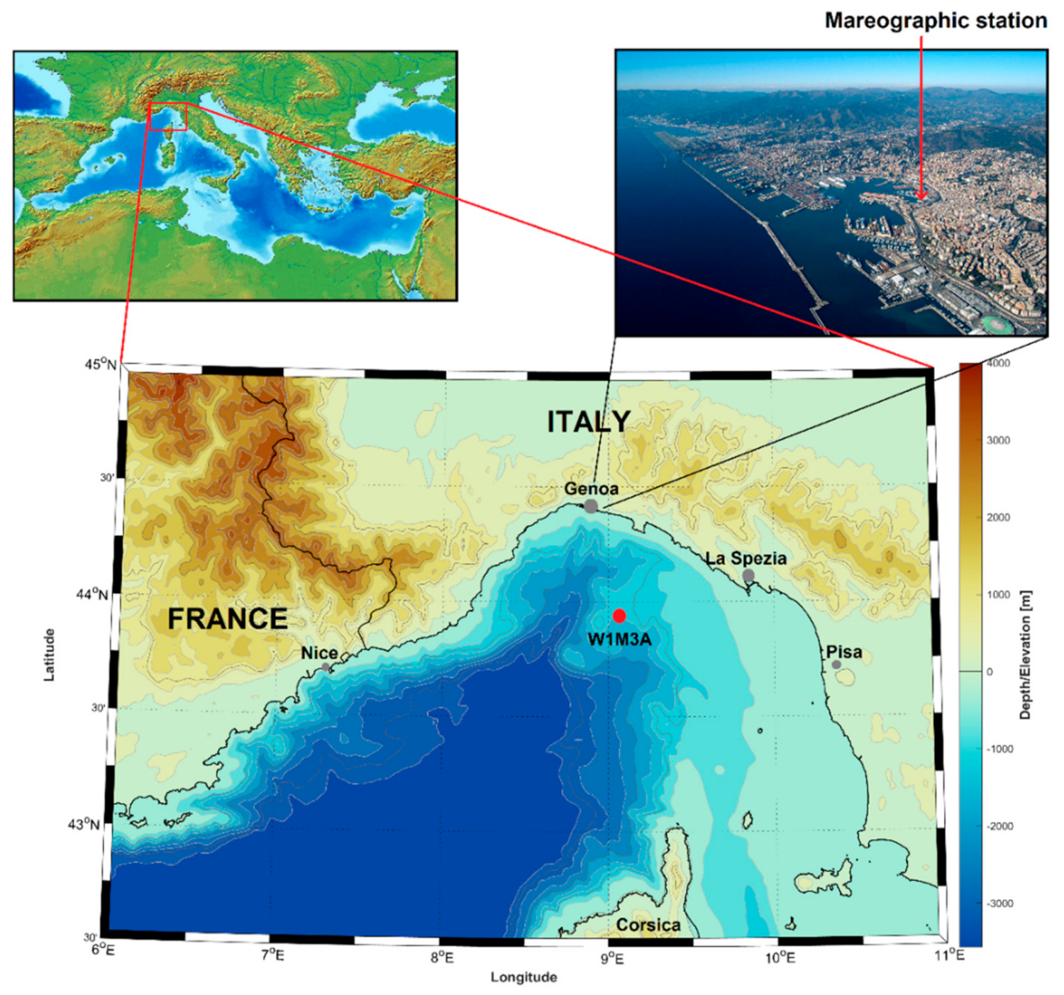
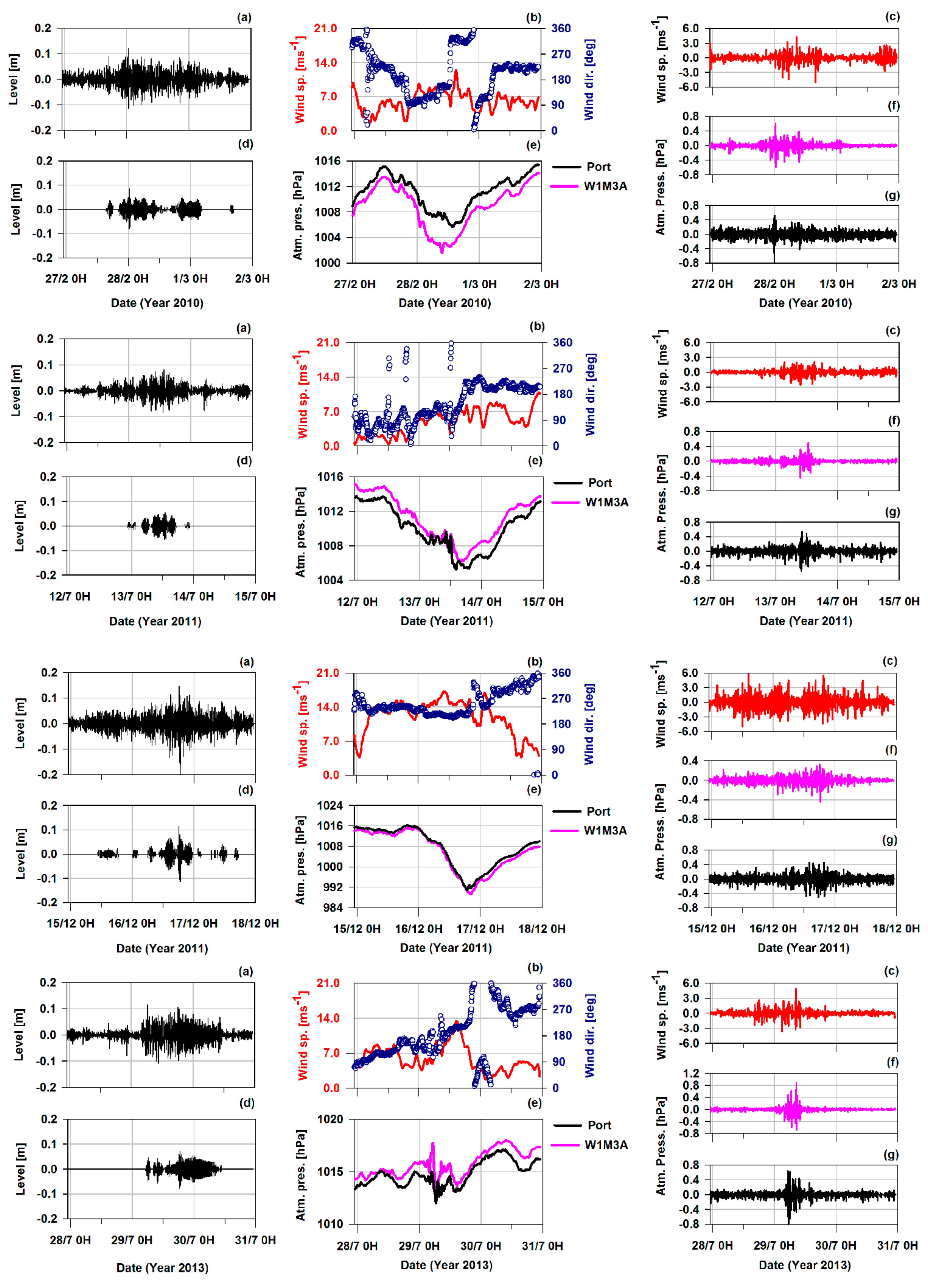
2.1. The Available Data-Set

Sea-level data used for this investigation were recorded in the port of Genoa (Ligurian Sea, Western Mediterranean, Figure 1). The tidal station (44°24’43.3”N–08°55’32.2”E), managed by the Italian Hydrographic Institute, has been collecting data since October 1883 and the mean sea-level, obtained from tide gauge measurements, is also the reference point of the Italian Height Network. A stilling well with an OTT HydroMet Thalimedes float operated, shaft encoder level sensor, an external OTT Radar Level Sensor 24 GHz radar level sensor and a non-contact radar pulse compose the tidal station. The accuracy of the sensors were 2 mm and 3 mm, respectively. Starting from August 2008, the sampling interval of both the instruments was set to one minute, thus allowing the analysis of short period sea-level oscillations. For this study, only the data from the float gauge were used, since the stilling well filters out small disturbances. However, radar sea-level measurements were used as a comparison for excluding possible damping effects or phase lag of the stilling well in the involved frequency band. The data-set from the tidal station also includes the atmospheric pressure measurements obtained by an OTT barometer having 0.1 hPa accuracy and sampling at a 5-minute time interval. Atmospheric pressure data were resampled at 1-minute time steps for a better comparison and clearer presentation with the correspondent sea-level data. Unfortunately, no wind data were available close to the station.

In order to eliminate spikes and bad data, the raw high frequency sea-level data were accurately checked and spline interpolation was applied to fill a few data lacks. On the contrary, longer time intervals of missing data, mainly due to routine maintenance, were not interpolated but filled with a constant value corresponding to the local mean sea-level. This allowed for the continuity of the time series, thus facilitating data processing without affecting the results of spectral analysis. On average, the missing or bad data were only about 0.3% of the entire time series. The data-set consisted of eight years of sea-level data, from 1 January 2009 to 31 December 2016. Data were grouped on a yearly basis and each annual time series was separately processed and analyzed (

Table 1. Number of missing or bad data for each year’s time series. Full time series of one-minute sample data are 525600 (527040 for leap year) long.

Year	Missing Data
2009	93
2010	273
2011	6887
2012	2380
2013	79
2014	2262
2015	870
2016	0

).

In order to evidence possible generation mechanisms of the identified tsunami-like episodes, the meteorological data acquired from the W1M3A observatory [37] were also used.

This meteo-oceanographic observatory is moored in the Ligurian Sea (43°49.25’N; 9°06.77’E) at a sea depth of 1200 m, about 40 nautical miles south of the port of Genoa, where sea-level data were collected. The position of the platform is an appropriate site to describe the meso-scale meteorological situation in the Central Ligurian Sea. The W1M3A observatory continuously collects meteorological parameters 10 m above the sea surface, as well as oceanographic physical and bio-geo-chemical parameters in the upper 40 m of the water column, thus fulfilling the concept of Essential Ocean Climate Variable. The system is one of the open ocean fixed platform of OceanSITES and it is part of both the M3A [38] and IFON network [39]. Atmospheric pressure, wind speed and direction time series were analyzed. The atmospheric pressure sensor was a Vaisala PTB100, having 0.3 hPa accuracy. Wind speed and direction were provided by a GILL Windsonic, with ± 2% and ± 2° at 12 ms⁻¹ accuracy, respectively. The acquisition system sampled the data at 2 Hz. Data in the first three months of 2009, in December 2014 and in the first three months of 2015, were missing, and they were not replaced by any interpolated value.

Further information was also obtained from the catalogue of earthquakes which occurred in the Mediterranean area, provided by the Italian Institute of Geophysics and Vulcanology (INGV), weather reports by the Regional Environmental Protection Agency of Liguria (ARPAL), and the consortium Laboratorio di Meteorologia Modellistica Ambientale (LaMMA). Moreover, public satellite images from the NASA’s Global Imagery Browse Services (GIBS), part of NASA’s Earth Observing System Data and Information System (EOSDIS) and from the archive of the European Organisation for the Exploitation of Meteorological Satellites (EUMETSAT) were used as additional support for the reconstruction of past synoptic situations.

2.2. Sea-Level Variability in the Gulf of Genoa

During the eight-year period of observations, the annual sea-level range (difference between the maximum and minimum) was between 77 cm and 95 cm, with a standard deviation of about 11 cm.

The contribution of the atmospheric pressure, computed as an inverse barometric effect, accounted for a variation between 43 cm and 57 cm with a standard deviation of about 8 cm.

The tidal regime in the Gulf of Genoa is semi-diurnal: The main tidal components (M2 and S2) have amplitudes of 8.5 cm and 3.2 cm respectively, and K1, the greatest diurnal component, at 3.6 cm [40]. The neap/spring modulation can reach 32 cm, and, even considering the annual component, the maximum observed tidal range never exceeds 47 cm.

Supra-tidal variability is characterized by the presence of the Ligurian Sea seiches [34,41,42]. The principal one has a period of 3.61 hours and contributes to the average frequency spectrum for less than one third of the quarter-diurnal tidal components (M4 and MS4); the three minor ones are in the band between the 2.9 and 2.1 hour period (Figure 2). Their overall contribution to sea-level variability is negligible as the amplitude of those waves is limited to few centimeters. At higher frequencies most of the energy is concentrated in the tsunami band, between 24–36 min.

Storm surges with high waves often hit the coasts and can be very dangerous, such as the extreme event of 29/30 October 2018, but coastal floods are very rare.

Despite the simultaneous occurrence of the maximal tidal range, and highest atmospheric pressure effect, the presence of a meteotsunami can lead to a sea-level range variation of more than ±50 cm, which occurred less than 9 hours during the whole examined period, representing about 0.1% of the total time. The percentage rises to 5% if the variation is ±40 cm.

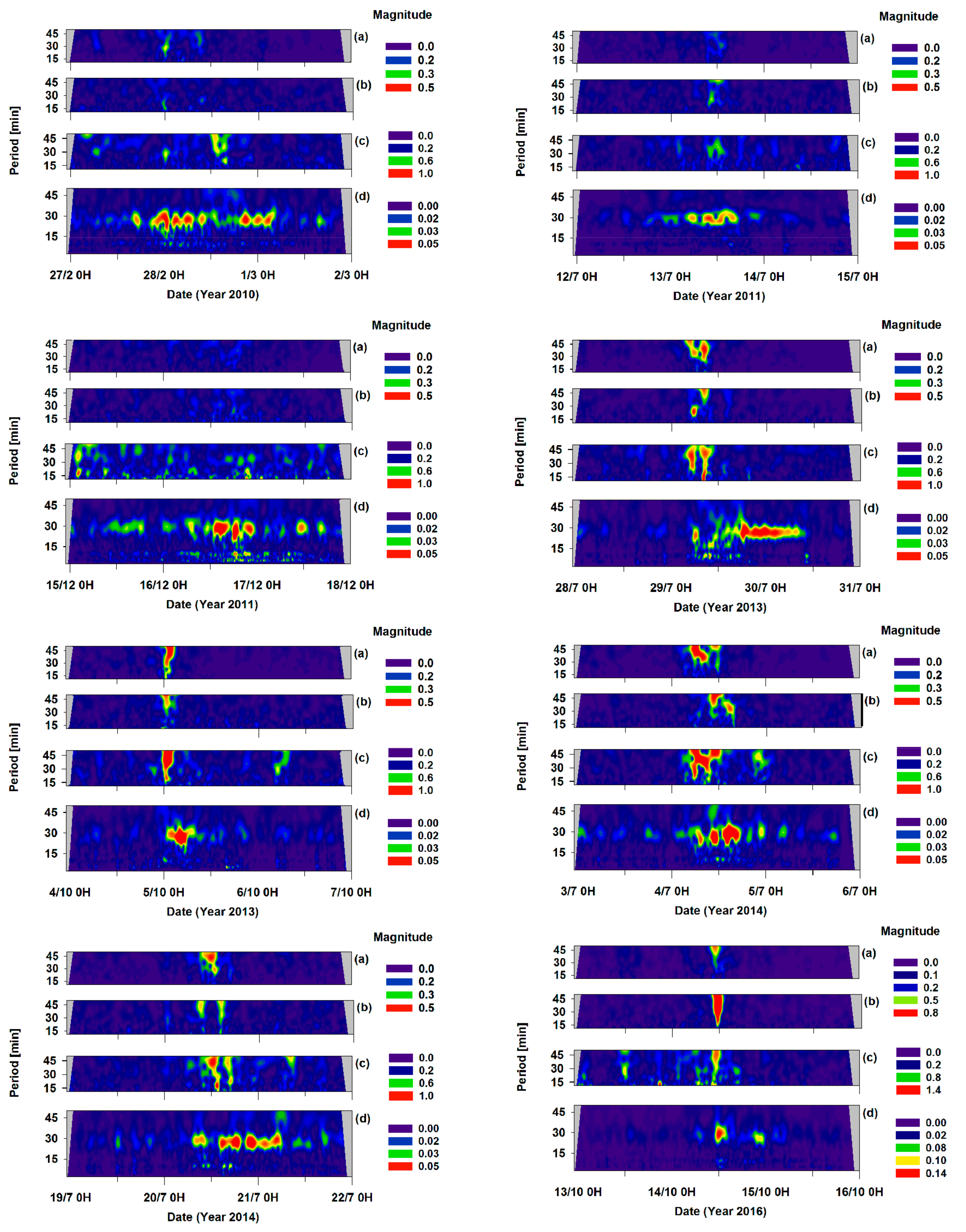
2.3. Event Detection by Time-Frequency Analysis

To filter out low frequency variability and tides, sea-level data were, firstly, smoothed using a quadratic least-square fit on 60 point (1 hour) moving window subsamples, and the center value of each sample was taken. Then, the resulting time series was subtracted from the original data, obtaining a de-trended time series that highlighted the supra-tidal variability. For each year, high resolution spectral analysis via fast Fourier transform (FFT) was applied to subsamples of 4096 data of the de-trended time series. The obtained spectra were averaged to lower the associated confidence level and to reduce the contribution of not persistent components. The resulting spectrum (Figure 3) evidences that the energy concentrated in the tsunami-band has its absolute maximum on 26.7 min and a secondary peak on 30.6 min. Minor peaks are at 45 min and 10 min, as well as in the swell band at 4–5 minutes.

Time frequency analysis [43,44,45] using a centered window 720 min wide and moving at 180 min steps was then performed on each yearly sample. The chosen window and overlap lengths were long enough to ensure adequate spectral resolution, and short enough to detect the occurrences of the events that, in some cases, lasted for just a few hours. Waves in the 26–30 minute band were a common feature of each spectrogram, and they were often associated with smaller amplitude oscillations with about 10 minutes periods.

From each yearly spectrogram, the time series of the amplitude in the band between 25.7 and 31.3 min were summed and the resulting time series were extracted for the analysis (Figure 4).

No important differences were found among averaged spectra from each year; they were all well correlated (correlation coefficient higher than 0.95) and the standard deviation was low. The inter-annual variability can be mostly ascribed to the different energy distribution on the main peaks. The 2016 spectrum had the greatest energy content: This was not only due to the main peak (26.7 min) but also due to the other frequencies. Furthermore, it revealed an important secondary peak centered at 29 min, which was less marked in other years. The lowest energy was in 2010, with a spectrum characterized by a maximum on 26.7 min and the rest of the energy in the tsunami band almost equally distributed.

Elevated energy values can be both associated to events characterized by the greatest amplitudes of the waves or a long persistence of the phenomenon. The greatest energy was detected on 14 October 2016, other relevant events occurred on July 2013, July 2014, and February 2015. During 2012, there were a huge numbers of events but they were all characterized by low energy. The analysis showed a significant inter-annual variability both in terms of number and intensity of the events.

The annual mean energy on the investigated frequency band normalized in respect to the 2016 value, shows the lowest values in 2009 and 2011 with less than 60%, 2010, 2012, and 2015 with about 70%, and 2013 and 2014 with the highest values, slightly more than 80%. The high variability in the occurrence and energy of the events is also evidenced by the standard deviation, which is about 60% higher than the mean energy in the whole period. 153 subsamples on a total of 23,352 analyzed by the spectrogram had more than one tenth of the maximum energy; 18 were higher than 30% and only four had energy higher than 60% of the main event (

Table 2. Distribution in classes of 0.1 amplitude of the normalized energy in the tsunami-band for the whole series (2009–2016) of analyzed subsamples.

Class	n
0–0.1	23198
0.1–0.2	108
0.2–0.3	26
0.3–0.4	13
0.4–0.5	3
0.5–0.6	0
0.6–0.7	1
0.7–0.8	2
0.8–0.9	0
0.9–1	1

).

The limited number of significant events does not clearly show a seasonal variability, although, excluding the event of October 2016, the highest peaks in spectrograms occurred more frequently in summer (July and August) and in February/March.

2.4. Earthquakes and Tsunami-like Oscillations

Earthquakes are known to be the primary cause of most destructive tsunamis. Nevertheless, as pointed out by Rabinovich [46] and Monserrat et al. [7], a spectral analysis of the ocean response in the tsunami-band frequency cannot give insights to its generation mechanism, as similar waves can be the result of earthquakes and submarine landslides or they can be storm-generated.

The tsunami generated by the earthquake of 23 February 1887 in the western Ligurian Sea (20 km off Imperia) and recorded by tide gauges in Genoa and Nice was probably the first tsunami registration in the Mediterranean Sea [47]. Along the coasts, close to the source area, waves reached an amplitude up to about 2 m, while the amplitudes recorded in Genoa did not exceed 40 cm. Analyzing more than 10 hour long records, the authors estimated the tsunami wave period to be about 22.5 min. Further investigations on barotropic response to coastal historical earthquakes in the Italian–French Riviera can be found in [48]. Resonant periods resulting from their numerical simulations were between 17 and 26 min for Genoa with wave amplitudes of a few centimeters.

To investigate about the possible causes of the identified episodes, the Mediterranean earthquakes recorded during 2009–2016 were analyzed. For the Mediterranean region, Masina et al. [3] estimate 3 h as the maximum time-lag from the occurrence of the earthquake and the tsunami appearance at coast. Furthermore, they suggest that tsunamis due to earthquakes with magnitudes less than six are hardly detectable in sea-level data.

The seismological archive provided by INGV reports that only 13 earthquakes of magnitude greater than 6 took place in the Mediterranean Sea between 2009 and 2016. For most of them, the epicenter was localized in the Eastern Basin, near the Greek coasts, while only one earthquake with magnitude of 6.3 occurred in the Western Basin, near the Strait of Gibraltar, facing the Moroccan coast, on 25 January 2016. In the Ligurian-Provencal basin, earthquakes have never exceeded magnitude 4. None of those earthquakes has produced detectable effects on the sea-level records in Genoa. Moreover, the archive does not indicate the occurrence of any tsunamigenic earthquake in the Mediterranean Sea in conjunction with the selected events. As consequence, the seismic origin can be excluded, and these events may be classified among the atmospherically induced shelf oscillations [7].

2.5. Wavelet Analysis

Standard Fourier transform is well localized only in the frequency domain since time information is completely lost due to the transformation to the frequency domain. A powerful tool to overcome this issue and to obtain a simultaneous localization both in time and frequency domains is represented by the wavelet transform which is particularly suitable for the analysis of tsunami-like oscillations, that are signals with time-varying amplitude and frequency [49,50].

Wavelets dilate so that the time component changes for different frequencies: The increase (decrease) of the time-window component involves a shift in the frequency towards high (low) frequency. Among others, a special family of complex-valued wavelet transforms for the analysis of oscillations is the analytic wavelet transform [51] that comprises the generalized Morse function whose frequency-domain form is expressed by Equation (1).

$$\mathsf{\Psi }\left(\mathsf{\omega }\right)=\mathrm{U}\left(\mathsf{\omega }\right){\mathrm{a}}_{\mathrm{P},\mathsf{\gamma }}{\mathsf{\omega }}^{\frac{{\mathrm{P}}^2}{\mathsf{\gamma }}}{\mathrm{e}}^{-{\mathsf{\omega }}^{\mathsf{\gamma }}}$$

(1)

$\mathrm{U}\left(\mathsf{\omega }\right)$ is the unitary step, ${\mathrm{a}}_{\mathrm{P},\mathsf{\gamma }}$ is a constant coefficient for normalization purposes, P² is the time-bandwidth product (${\mathrm{P}}^2=\mathsf{\beta }\mathsf{\gamma }$) where β is the decay or compactness parameter and $\mathsf{\gamma }$ is the symmetry parameter for Morse wavelet in time through the demodulate skewness [52]. The choice of P² and $\gamma$ defines the shape of the wavelet and it is responsible for the behavior of the transform itself. An increase of the time-bandwidth parameter implies a wavelet more spread out in time and narrower in frequency.

Furthermore, the time-bandwidth product, which is proportional to the wavelet’s duration in time, allows for the definition of the number of oscillations that can fit into the time-domain wavelet’s centered window at its peak frequency that is defined as Equation (2).

$${\omega }_{pk}={\left(\frac{P^2}{\gamma }\right)}^{\raisebox{1ex}{$1$}\!\left/ \!\raisebox{-1ex}{$\gamma $}\right.}$$

(2)

The standard deviation of the Morse wavelet can be approximately estimated as $\sqrt{\frac{P^2}{2}}$ in time and $\frac{1}{2}\sqrt{\frac{2}{P^2}}$ in frequency.

Sea-level data corresponding to the most significant tsunami-like events identified through FFT based time-frequency analysis, as well as the correspondent pressure and wind data, were processed by wavelet transform. The chosen Morse function parameters were $\gamma$= 3 and P² = 120 in order to minimize the Heisenberg area, maintaining a perfect symmetry in the frequency domain and to maximize the precision of the localization in the frequency domain. The uncertainty can be estimated at about 10 minutes in time and about 0.07 Hz in frequency.

In order to filter out noise and uninteresting oscillations, the obtained scalograms of sea level data were filtered, excluding all values lower than the 40% of the absolute maximum value of wavelet transform, considering the whole analyzed period (2009–2016). Then, the filtered time series of the tsunami-like oscillations were reconstructed applying the inverse wavelet transform [53] and using the same parameters of the direct transform (Morse function, $\gamma$ = 3 and P² = 120). In this way, it was possible to clearly identify the patterns associated to each instance of tsunami-like oscillation analyzed.

3. Results and Discussion

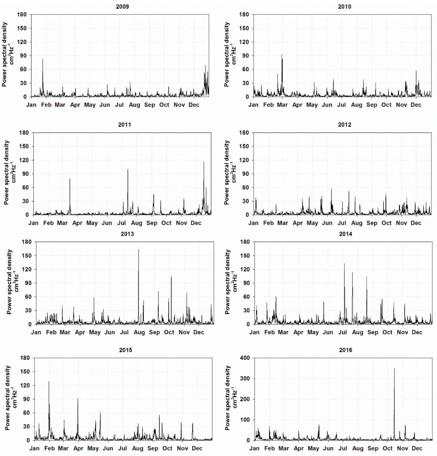
3.1. Temporal Evolution Patterns’ Characterization

The time-frequency analysis allows evidencing the events with the highest energy or with peculiar characteristics. These were selected and investigated in terms of frequency and temporal evolution pattern provided through wavelet analysis (Figure 5). Often, the obtained signals showed a superimposition of several patterns that differ in duration, peak magnitude and base surface in time-frequency domain, underlying volume and time lapse, although the dominant frequency was at 26.7 minutes.

Impulse-like response [6] can be well identified in the event of 14 October 2016. The temporal evolution of the signal is characterized by a response to a single impulse, with the first wave reaching the greatest amplitude and the others rapidly dampening and having decreasing frequencies. On the other hand, the event that took place on 29 July 2013 and lasted 30 hours was characterized by a constant dominant frequency, a short intense wave train accompanied by a long oscillatory tail with amplitude slowly decreasing with the time.

Most of the events (e.g., February 2010, July 2011, July 2014) displayed a series of eye-shaped bursts close to each other: The simultaneous presence of the two main-mode oscillations having close periods (26.7 and 30.6 min) gives way to beats, which are consistent with the evidenced signal modulation.

This two-mode shelf oscillation of the Ligurian Sea was described by Papa [35], who investigated the barotropic response of the Ligurian Sea to random atmospheric disturbances on the open boundaries by using a Northern Emisphere (NH) barotropic model at 10 km resolution [42,54]. He analyzed the spectrum of the sea-level elevation in grid points close to Genoa and found two close frequencies of 2.22 cph and 2.36 cph (27 min and 25.2 min) with estimated amplitudes of 9 cm and 6 cm, respectively. Despite the simple models available at that period and the coarse spatial resolution used, the qualitative results were consistent with the observed data.

Considering 200 m depth as the limit for the shelf, its mean width close to Genoa is only about 6.5 km. Using the simple Merian’s formula for an open system, $\mathrm{T}=4\mathrm{L}/\sqrt{\mathrm{gh}}$, where L is the shelf width, g is the acceleration of gravity and h is the mean shelf depth, the estimated fundamental mode oscillation period T was about 10 min. This shelf oscillation period is consistent with the minor peak evidenced in the spectral analysis, but does not explain the main energy on the lower frequencies, which probably involves a wider area.

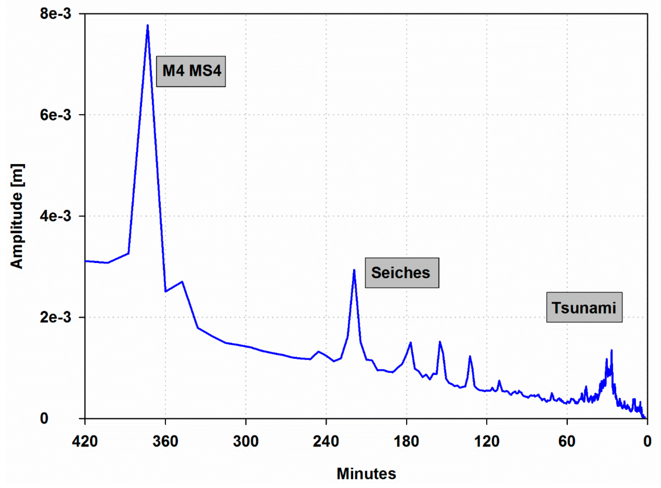
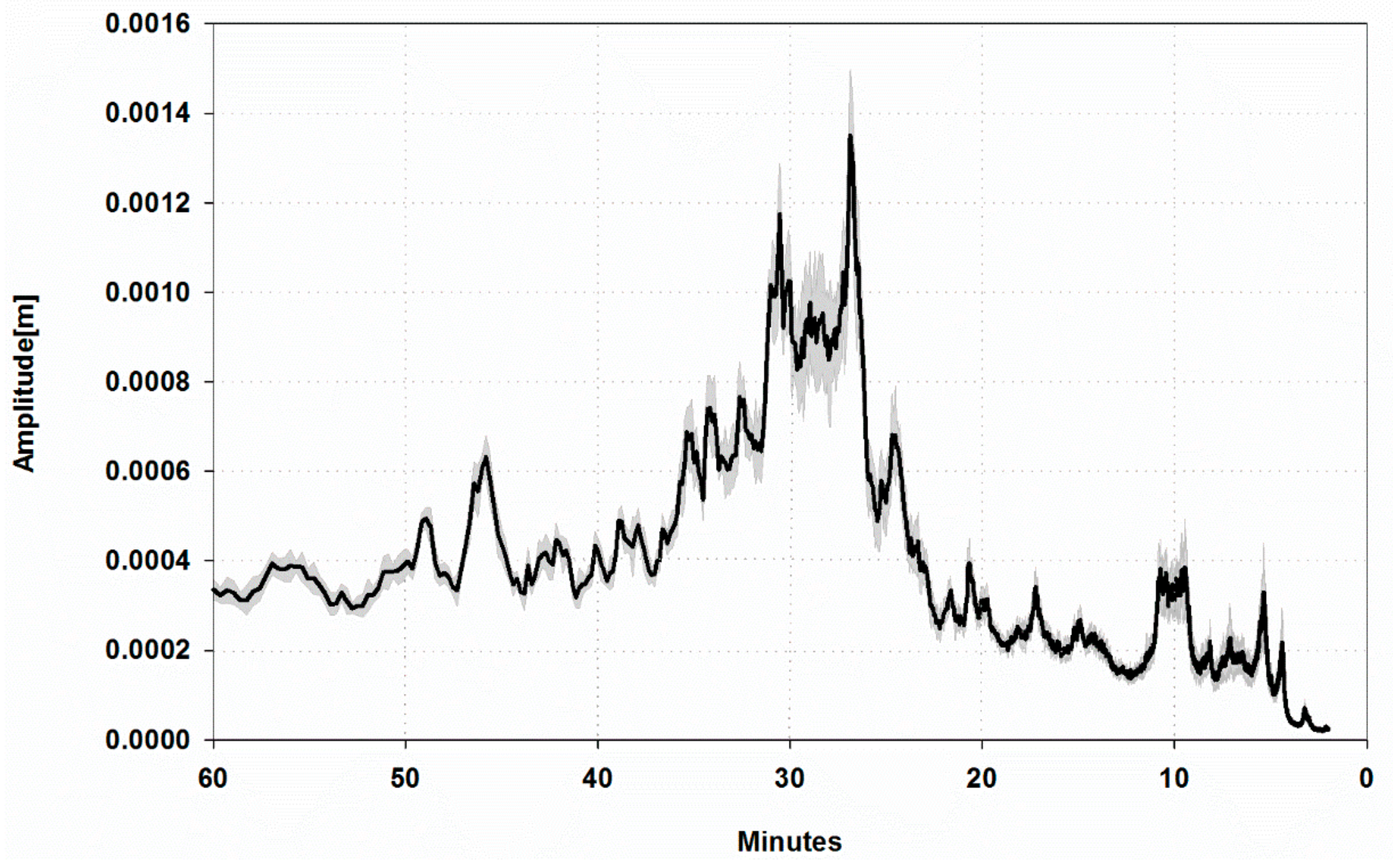
3.2. Event Description

The available atmospheric pressure data measured by the barometer of the mareographic station and the meteorological parameters collected on the W1M3A observatory, as well as the mesoscale synoptic situation were analyzed for each of the selected events (Figure 6 and Figure 7).

The first event occurred between 27 February and 1 March 2010, when the very violent cyclone Xynthia hit the northwestern Europe [55]. The northwestern Mediterranean Sea was also affected by the currents generated by this powerful vortex, with a cloud storm extending from Atlantic Ocean to Portugal, Spain, France, and Northern Italy. A pressure minimum developed over the Ligurian basin. The wind exceeded 50 kmh⁻¹ in the open sea and on the coast, up to 70 kmh⁻¹ over the high ground west of the Gulf of Genoa (Monte di Portofino). Starting from the night of 28 February, when the pressure began to decrease and the wind turn, the sea level data showed a long series of oscillations, even if of relatively small amplitude, ending at the beginning of 1 March. The wavelet analysis suggests that this event can be attributed to disturbances of both atmospheric pressure and wind. At first, the rapid and discontinuous drop of pressure dominated, while, as soon as it started to increase again, the contribution of the wind prevailed.

Although of significantly lower intensity, the wavelet analysis of the sea-level relative to the event of 13 July 2011 displayed very similar characteristics. The atmospheric disturbances were linked to a flow of cold air from the north east over the warm Ligurian Sea, generating strong instability and violent thunderstorms. Surface pressure data reflect these disturbances with significant changes in less than 1 hour, especially around midday, which are more marked on the coast than in the open sea, as confirmed by the wavelet analysis. Nevertheless, high frequency data (5 sec) recorded on the W1M3A platform shows the presence of a jump over 4 hPa in less than 8 minutes, that the 5 minutes average dampened.

Western winds exceeding 70 kmh⁻¹ and a storm with waves over 6 m hit the coast of the Gulf of Genoa, an event of 16 December 2011. This situation was caused by the passage of a deep low from France, accompanied by a flow of Arctic air, and by the strong baric gradient between the Algerian coast and the Ligurian basin. The meteorological data shows a fast atmospheric pressure drop of more than 24 hPa in less than 24 h and the strong westerly wind lasting more than 48 h. The wavelet analysis of the sea-level data shows a long series of bursts of oscillations, particularly intense compared to the pressure minimum passage. Furthermore, it evidences the presence of oscillations at the frequency of 10 min. The wavelet analysis of surface meteorological parameters show some features from only the wind, but there is not a clear correspondence with the sea level oscillations.

On 29 July 2013, the fast eastward passage of a cold front over the warm Ligurian Sea generated atmospheric disturbances, well evident in the two pressure datasets. From early morning to late afternoon, atmospheric pressure were subject to frequent jumps of less than 2 hPa in 5 min, higher on the observatory than on the coast. The wavelet analysis highlights oscillations with greater magnitude over the open sea. At the same time, the wind increased and rotated from east to south-southwest. When the pressure began to increase, the wind rapidly diminished, turning to the north. The phenomenon ended on the evening of the 30 July. The spectrogram of the corresponding sea-level data shows a particularly high peak. The analysis of the sea-level time series does not evidence relevant wave amplitudes, which hardly exceeded ten centimeters, but did show an impressive persistence of the oscillations, lasting for more than 30 hours. Initially, the signal is weak, but, after reaching the maximum amplitude, the development of waves having a period of 26.7 min is well evident. It must be noted that this occurs when the wind decreases and turns towards north. These may be favorable requirements for a swell-dominated condition, as Pattiaratchi and Wijeratne [56] described when they investigated meteotsunami mechanisms on the Australian coasts.

On 5 October 2013, a well-marked pressure jump was recorded almost simultaneously at the W1M3A observatory and in the port. This occurred immediately after a fast pressure decrease started in the late night of the previous day and due to the arrival of an Atlantic perturbation. The wind turned from south east to north west and increased. The wavelet analysis of both the wind and the two pressure data sets provide evidence for the occurrence of the jump and the contemporaneous sea level oscillations in the tsunami band. These patterns are very similar to those obtained for the event of October 2016, even if of less magnitude.

The synoptic situation on 4 July 2014 was characterized by a wide cut-off over Spain, moving eastward, and with an intense south flow over the Ligurian Sea, which created high instability and gave rise to convective systems along the coast. Until the early afternoon, the surface pressure data show a continuous series of oscillations; the ones with greater amplitude were recorded over the open sea. Furthermore, the wavelet analysis shows that the pressure disturbance moved from the open sea to the coast. The sea-level oscillations in the tsunami band co-occured during the whole period of the atmospheric pressure disturbances. Their magnitude seems to increase with the passage of the perturbation and the consequent changes of wind direction.

In the night between 19 and 20 July 2014, the approach of a North Atlantic cold front to the Ligurian basin, already affected by an intense warm and wet flow of Saharan origin, created conditions of strong instability, favoring the development of convective systems and, on 21 July, an occlusion on the basin with a minimum of about 1005 hPa. Although the surface pressure dropped slowly during the day, numerous oscillations were detected in both the pressure data sets. The most significant took place in the early afternoon, with variations of about 4 hPa in less than 1.5 hours. Starting from the morning of the 20 July, bursts of small sea-level amplitudes were observed for about 24 hours and seemed to follow that trend.

The event of 14 October 2016 is the most relevant in the whole examined time series for the wave amplitude. A clear pressure jump is evident in the pressure data, more marked in the time series recorded in the port than in the offshore one. Furthermore, the measurements from the W1M3A observatory show a similar jump in the wind speed while its direction undergoes a complete rotation in less than 1 hour. The synoptic situation, described in the weather reports and well visible in satellite images (Figure 8), was characterized by an Atlantic low-pressure system that moved eastward, allowing a meridional flow of warm and wet air from the African coast on the Ligurian Sea. When cold air from the Po Valley passed over the Appenines, it triggered a large convective system over the Ligurian Sea. A squall line, extended from Corsica to the Alps and with axis in the southwest–northeast direction, moved fast towards the Genoese coast and hit Genoa at around 12:00. A powerful wet macroburst developed near the Tigullio Gulf. Parodi et al. [57] estimated that the affected area was about 30 km long and 10 km wide. The wind gusts reached a speed greater than 110 kmh^-1, while the atmospheric pressure decreased from 1010 to 1005 hPa in less than three hours, followed by an impressive rise to 1016 hPa in a few minutes [58]. Two hours later, it decreased to 1010 hPa and remained almost constant during the rest of the event. The surface meteorological sensors on the W1M3A observatory started to detect the cold front on the Ligurian Sea since the late night of 13 October. The wavelet analysis of the pressure data show that the oscillations have the highest magnitude in correspondence with the pressure jumps. The oscillations of the sea-level coincide quite well with such atmospheric disturbances.

The ocean response was impulse-like and lasted about three hours. The time-lag between the first wave and the arrival of the pressure jump was below the 5 minutes sampling interval of the local atmospheric pressure measurements and the highest crest to trough amplitude was 50 cm, about five times the amplitude of the inverse barometric effect. After only a few hours wave amplitudes rapidly damped. At the beginning of the event, the spectrum was noisy, with the energy distributed in a broad band, between 25 and 45 min, then shifted towards a neater frequency close to the period of 28.8 min.

4. Concluding Remarks

Eight years of high-frequency sea-level data in the Gulf of Genoa were analyzed to investigate the occurrence and characteristics of meteotsunamis and their potential hazards. To this end, time-frequency analysis has proven to be an efficient method to process long-term timeseries data for preliminary and objective events detection. Results show that long periods of waves in the tsunami band often occur and account for a huge part of the supra-tidal variability. They are related to a wide variety of atmospheric disturbances, mostly due to the passage of a low pressure system and a cold front on the Ligurian basin, determining conditions of strong instability. Frequently, atmospheric gravity waves are linked to similar patterns [59,60,61,62,63,64]. The number and intensity of these meteotsunamis strongly differ from one year to another and, although the time series is not long enough for a significant statistical analysis, a slight increasing trend in the recent years may have been detected. There is no a clear evidence of a particular seasonality; nevertheless, a high number of events are recorded on July, when the strongest air-sea interaction favors the development of intense mesoscale convective systems [65].

The most significant event of 14 October 2016 has a clear relation with the pressure jump which affected a localized area in the Ligurian Sea. This impressive pressure jump reminds one of what was described by Jansà et al. [22] regarding the meteorological tsunami which occurred on Menorca on 15 June 2006. The availability of atmospheric pressure data collected from the W1M3A observing system, located 37 nautical miles far from the coast, as well as satellite images, allowed the estimation of the speed of the atmospheric pressure disturbance propagation—about 30 ms⁻¹. Considering an average shelf depth of 100 m, the shallow-water wave speed was 31 ms⁻¹. That meteotsunami can be explained in terms of Proudman resonance induced by the pressure jump as described for other similar events [20,66]; moreover, the observed resonant amplification factor was consistent with the estimated values.

Local atmospheric disturbances close to the coast play a major role in generating meteotsunamis in the Gulf of Genoa. In fact, several significant pressure oscillations measured only in the open sea do not affect the sea-level data collected in the port. Furthermore, the large-scale atmospheric disturbances which crossed the whole Mediterranean and Black Sea area from 23 to 27 June 2014, giving origin to meteotsunami episodes detected at several coastal places [33], had negligible effects in the Gulf of Genoa. Only small amplitude waves having a noisy spectrum were observed on 25 and 26 June in the sea-level measurements, consistent with the low Froude number (0.1) estimated by the authors. Moreover, the wind speed measured by W1M3A was quite low, in agreement with the synoptic maps showing the main perturbation passing south of the platform, far from the coasts of the Gulf of Genoa. On 27 July 2012, when meteotsunamis developed in the north-western Mediterranean basin were detected along the Spanish and French coasts by the RONIM mareographic network (SHOM, 2012), the wave’s amplitude, detected by the measurements in Genoa, did not exceed five centimeters. Among the large scale synoptic situations responsible for meteotsunamis generation in the Mediterranean area and reported by Šepic et al. [33], only the one on 19/20 July 2011 (not described here) slightly affected the Ligurian Sea: Low-amplitude (4–5 cm), but well developed oscillations at the two main identified frequencies were persistent for several hours.

Despite the strong air-sea thermal contrast and the complex orography of the Ligurian Sea, characterized by the presence of mountains over 2000 m high and only few kilometers away from the coastline, well support the atmospheric conditions suitable for meteotsunami generation [67,68], the topography of Gulf of Genoa generally prevents destructive tsunamis’ propagation.

Nevertheless, meteotsunamis having amplitudes of about 10–15 cm often occur and, in a few cases, their amplitude is significantly greater than the main tidal component. Compared with the less than 1 m average range of sea-level variation in the port of Genoa, a meteotsunami having an amplitude of 30/40 cm can significantly contribute to this variation. From the perspective of climate change with the related sea-level rise, along with the increasing size of ships, the variation may impact the maximum vessel draught, and should be taken into consideration for safe navigation and coastal structure protection.

References

1. Bernard, E.; Titov, V. Evolution of tsunami warning systems and products. Philos. Trans. R. Soc. A Math. Phys. Eng. Sci. 2015, 373, 20140371. [Google Scholar] [CrossRef] [PubMed]
2. Maramai, A.; Brizuela, B.; Graziani, L. The Euro-Mediterranean Tsunami Catalogue. Ann. Geophys. 2014. [Google Scholar] [CrossRef]
3. Masina, M.; Archetti, R.; Besio, G.; Lamberti, A. Tsunami taxonomy and detection from recent Mediterranean tide gauge data. Coast. Eng. 2017, 127, 145–169. [Google Scholar] [CrossRef]
4. Tinti, S.; Armigliato, A.; Bortolucci, E.; Piatanesi, A. Identification of the source fault of the 1908 Messina earthquake through tsunami modelling. Is it a possible task? Phys. Chem. Earth Part B Hydrol. Oceans Atmos. 1999, 24, 417–421. [Google Scholar] [CrossRef]
5. Heidarzadeh, M.; Necmioglu, O.; Ishibe, T.; Yalciner, A.C. Bodrum–Kos (Turkey–Greece) Mw 6.6 earthquake and tsunami of 20 July 2017: A test for the Mediterranean tsunami warning system. Geosci. Lett. 2017, 4, 31. [Google Scholar] [CrossRef]
6. Rabinovich, A.B.; Monserrat, S. Meteorological tsunamis near the Balearic and Kuril Islands: Descriptive and statistical analysis. Nat. Hazards 1996, 13, 55–90. [Google Scholar] [CrossRef]
7. Monserrat, S.; Vilibić, I.; Rabinovich, A.B. Meteotsunamis: Atmospherically induced destructive ocean waves in the tsunami frequency band. Nat. Hazards Earth Syst. Sci. 2006, 6, 1035–1051. [Google Scholar] [CrossRef]
8. Thomson, R.E.; Rabinovich, A.B.; Fine, I.V.; Sinnott, D.C.; McCarthy, A.; Sutherland, N.A.S.; Neil, L.K. Meteorological tsunamis on the coasts of British Columbia and Washington. Phys. Chem. Earth Parts A/B/C 2009, 34, 971–988. [Google Scholar] [CrossRef]
9. Pattiaratchi, C.B.; Sarath Wijeratne, E.M. Tide Gauge Observations of 2004–2007 Indian Ocean Tsunamis from Sri Lanka and Western Australia. Pure Appl. Geophys. 2009, 166, 233–258. [Google Scholar] [CrossRef]
10. Proudman, J. The Effects on the Sea of Changes in Atmospheric Pressure. Geophys. J. Int. 1929, 2, 197–209. [Google Scholar] [CrossRef]
11. Hibiya, T.; Kajiura, K. Origin of theAbiki phenomenon (a kind of seiche) in Nagasaki Bay. J. Oceanogr. Soc. Japan 1982, 38, 172–182. [Google Scholar] [CrossRef]
12. Greenspan, H.P. The generation of edge waves by moving pressure distributions. J. Fluid Mech. 1956, 1, 574–592. [Google Scholar] [CrossRef]
13. Monserrat, S.; Rabinovich, A.B.; Casas, B. On the reconstruction of the transfer function for atmospherically generated seiches. Geophys. Res. Lett. 1998, 25, 2197–2200. [Google Scholar] [CrossRef] [Green Version]
14. Pattiaratchi, C.B.; Wijeratne, E.M.S. Are meteotsunamis an underrated hazard? Philos. Trans. R. Soc. A Math. Phys. Eng. Sci. 2015, 373, 20140377. [Google Scholar] [CrossRef] [PubMed] [Green Version]
15. Vilibić, I. Numerical study of the Middle Adriatic coastal waters’ sensitivity to the various air pressure travelling disturbances. Ann. Geophys. 2005, 23, 3569–3578. [Google Scholar] [CrossRef]
16. Šepić, J.; Vilibić, I.; Belušić, D. Source of the 2007 Ist meteotsunami (Adriatic Sea). J. Geophys. Res. 2009, 114. [Google Scholar] [CrossRef]
17. Šepić, J.; Vilibić, I.; Fine, I. Northern Adriatic meteorological tsunamis: Assessment of their potential through ocean modeling experiments: Northern Adriatic meteotsunamis. J. Geophys. Res. Oceans 2015, 120, 2993–3010. [Google Scholar] [CrossRef]
18. Vilibić, I.; Šepić, J. Destructive meteotsunamis along the eastern Adriatic coast: Overview. Phys. Chem. Earth Parts A/B/C 2009, 34, 904–917. [Google Scholar] [CrossRef]
19. Šepić, J.; Vilibić, I. The development and implementation of a real-time meteotsunami warning network for the Adriatic Sea. Nat. Hazards Earth Syst. Sci. 2011, 11, 83–91. [Google Scholar] [CrossRef] [Green Version]
20. Vilibić, I.; Šepić, J.; Rabinovich, A.B.; Monserrat, S. Modern Approaches in Meteotsunami Research and Early Warning. Front. Mar. Sci. 2016, 3. [Google Scholar] [CrossRef] [Green Version]
21. Denamiel, C.; Šepić, J.; Ivanković, D.; Vilibić, I. The Adriatic Sea and Coast modelling suite: Evaluation of the meteotsunami forecast component. Ocean Model. 2019, 135, 71–93. [Google Scholar] [CrossRef]
22. Jansa, A.; Monserrat, S.; Gomis, D. The rissaga of 15 June 2006 in Ciutadella (Menorca), a meteorological tsunami. Adv. Geosci. 2007, 12, 1–4. [Google Scholar] [CrossRef] [Green Version]
23. Vilibić, I.; Monserrat, S.; Rabinovich, A.; Mihanović, H. Numerical Modelling of the Destructive Meteotsunami of 15 June, 2006 on the Coast of the Balearic Islands. Pure Appl. Geophys. 2008, 165, 2169–2195. [Google Scholar] [CrossRef]
24. Marcos, M.; Monserrat, S.; Medina, R.; Orfila, A.; Olabarrieta, M. External forcing of meteorological tsunamis at the coast of the Balearic Islands. Phys. Chem. Earth Parts A/B/C 2009, 34, 938–947. [Google Scholar] [CrossRef] [Green Version]
25. Renault, L.; Vizoso, G.; Jansá, A.; Wilkin, J.; Tintoré, J. Toward the predictability of meteotsunamis in the Balearic Sea using regional nested atmosphere and ocean models: TOWARD THE METEOTSUNAMIS PREDICTABILITY. Geophys. Res. Lett. 2011, 38. [Google Scholar] [CrossRef]
26. Orlić, M. About a possible occurrence of the Proudman resonance in the Adriatic. Prelim. Commun. 1980, 16, 79–88. [Google Scholar]
27. Orlić, M.; Belušić, D.; Janeković, I.; Pasarić, M. Fresh evidence relating the great Adriatic surge of 21 June 1978 to mesoscale atmospheric forcing. J. Geophys. Res. 2010, 115. [Google Scholar] [CrossRef] [Green Version]
28. Colucci, P.; Michelato, A. An approach to the study of the “Marrubbio” phenomenon. Boll. Di Geofis. Teor. Ed Appl. 1976, 19, 3–10. [Google Scholar]
29. Candela, J.; Mazzola, S.; Sammari, C.; Limeburner, R.; Lozano, C.J.; Patti, B.; Bonanno, A. The “Mad Sea” Phenomenon in the Strait of Sicily. J. Phys. Oceanogr. 1999, 29, 2210–2231. [Google Scholar] [CrossRef]
30. Šepić, J.; Vilibić, I.; Rabinovich, A.; Tinti, S. Meteotsunami (“Marrobbio”) of 25–26 June 2014 on the Southwestern Coast of Sicily, Italy. Pure Appl. Geophys. 2018, 175, 1573–1593. [Google Scholar] [CrossRef]
31. Gravili, D.; Napolitano, E.; Pierini, S. Barotropic aspects of the dynamics of the Gulf of Naples (Tyrrhenian Sea). Cont. Shelf Res. 2001, 21, 455–471. [Google Scholar] [CrossRef]
32. Bressan, L.; Tinti, S. Statistical properties of coastal long waves analysed through sea-level time-gradient functions: Exemplary analysis of the Siracusa, Italy, tide-gauge data. Nat. Hazards Earth Syst. Sci. 2016, 16, 223–237. [Google Scholar] [CrossRef]
33. Šepić, J.; Vilibić, I.; Lafon, A.; Macheboeuf, L.; Ivanović, Z. High-frequency sea level oscillations in the Mediterranean and their connection to synoptic patterns. Prog. Oceanogr. 2015, 137, 284–298. [Google Scholar] [CrossRef]
34. Caloi, P.; Spadea, M.C. Studio preliminare sulle oscillazioni libere del Golfo di Genova. Ann. Geophys. 2011, 1, 107–117. [Google Scholar]
35. Papa, L. A numerical verification of a shelf oscillation in the Gulf of Genoa. Oceanol. Acta 1981, 4, 11–12. [Google Scholar]
36. Denamiel, C.; Šepić, J.; Vilibić, I. Impact of Geomorphological Changes to Harbor Resonance During Meteotsunamis: The Vela Luka Bay Test Case. Pure Appl. Geophys. 2018, 175, 3839–3859. [Google Scholar] [CrossRef]
37. Canepa, E.; Pensieri, S.; Bozzano, R.; Faimali, M.; Traverso, P.; Cavaleri, L. The ODAS Italia 1 buoy: More than forty years of activity in the Ligurian Sea. Prog. Oceanogr. 2015, 135, 48–63. [Google Scholar] [CrossRef]
38. Bozzano, R.; Pensieri, S.; Pensieri, L.; Cardin, V.; Brunetti, F.; Bensi, M.; Petihakis, G.; Tsagaraki, T.M.; Ntoumas, M.; Podaras, D.; et al. The M3A network of open ocean observatories in the Mediterranean Sea. In Proceedings of the 2013 MTS/IEEE OCEANS—Bergen, Bergen, Norway, 10–14 June 2013; pp. 1–10. [Google Scholar]
39. Ravaioli, M.; Bergami, C.; Riminucci, F.; Langone, L.; Cardin, V.; Di Sarra, A.; Aracri, S.; Bastianini, M.; Bensi, M.; Bergamasco, A.; et al. The RITMARE Italian Fixed-Point Observatory Network (IFON) for marine environmental monitoring: A case study. J. Oper. Oceanogr. 2016, 9, s202–s214. [Google Scholar] [CrossRef]
40. Istituto Idrografico della Marina Tavole Di Marea E Delle Correnti Di Marea Venezia E Stretto Di Messina; Istituto Idrografico della Marina: Genova, Italy, 2014; p. 3133.
41. Papa, L. A numerical and statistical investigation of a seiche oscillation of the Ligurian Sea. Deutsch. Hydrogr. Z. 1981, 34, 15–25. [Google Scholar] [CrossRef]
42. Papa, L. A short period rotating seiche of the Ligurian SEa. Oceanol. Acta 1984, 7, 1–4. [Google Scholar]
43. Guedes Soares, C.; Cherneva, Z. Spectrogram analysis of the time–frequency characteristics of ocean wind waves. Ocean Eng. 2005, 32, 1643–1663. [Google Scholar] [CrossRef]
44. Picco, P.; Cappelletti, A.; Sparnocchia, S.; Schiano, M.E.; Pensieri, S.; Bozzano, R. Upper layer current variability in the Central Ligurian Sea. Ocean Sci. 2010, 6, 825–836. [Google Scholar] [CrossRef]
45. Picco, P.; Demarte, M.; D’Epifanio, R.; Guideri, M.; Repetti, L.; Morucci, S.; Ferla, M. Detection of short-period sea level oscillations in the Gulf of Genoa. In Proceedings of the OCEANS 2017—Aberdeen, Aberdeen, UK, 19–22 June 2017; pp. 1–4. [Google Scholar]
46. Rabinovich, A.B. Spectral analysis of tsunami waves: Separation of source and topography effects. J. Geophys. Res. Oceans 1997, 102, 12663–12676. [Google Scholar] [CrossRef]
47. Eva, C.; Rabinovich, A.B. The February 23, 1887 tsunami recorded on the Ligurian Coast, western Mediterranean. Geophys. Res. Lett. 1997, 24, 2211–2214. [Google Scholar] [CrossRef]
48. Pelinovsky, E.; Kharif, C.; Riabov, I.; Francius, M. Study of tsunami propagation in the Ligurian Sea. Nat. Hazards Earth Syst. Sci. 2001, 1, 195–201. [Google Scholar] [CrossRef]
49. Emery, W.J.; Thomson, R.E. Data Analysis Methods in Physical Oceanography, 2nd and rev. ed.; Elsevier: Amsterdam, The Netherlands; New York, NY, USA, 2001; ISBN 978-0-444-50756-3. [Google Scholar]
50. Keller, W. Wavelets in Geodesy and Geodynamics; De Gruyter: Berlin, Germany, 2008; ISBN 978-3-11-019818-8. [Google Scholar]
51. Mallat, S.G. A Wavelet Tour of Signal Processing; Academic Press: San Diego, CA, USA, 1998; ISBN 978-0-12-466605-4. [Google Scholar]
52. Lilly, J.M.; Olhede, S.C. Higher-Order Properties of Analytic Wavelets. IEEE Trans. Signal Process. 2009, 57, 146–160. [Google Scholar] [CrossRef]
53. Incardone, S. Hydrographic Data Analysis: Wavelet Filter Applications. In Post Graduate Master Degree on Marine Geomatics, Advanced Technologies Applied to Marine Environment, University of the Study of Genoa; University of Genoa: Genoa, Italy, 2017. [Google Scholar]
54. Papa, L. The free oscillations of the Ligurian Sea computed by the H-N method. Deutsch. Hydrogr. Z. 1977, 30, 81–90. [Google Scholar] [CrossRef]
55. Liberato, M.L.R.; Pinto, J.G.; Trigo, R.M.; Ludwig, P.; Ordóñez, P.; Yuen, D.; Trigo, I.F. Explosive development of winter storm Xynthia over the subtropical North Atlantic Ocean. Nat. Hazards Earth Syst. Sci. 2013, 13, 2239–2251. [Google Scholar] [CrossRef] [Green Version]
56. Pattiaratchi, C.; Wijeratne, E.M.S. Observations of meteorological tsunamis along the south-west Australian coast. Nat. Hazards 2014, 74, 281–303. [Google Scholar] [CrossRef] [Green Version]
57. Parodi, A.; Gallus, W.; Maugeri, M.; Turato, B. Observational and modelling study of a major downburst event in Liguria: The Portofino case on 14 October 2016. In Proceedings of the Geophysical Research Abstracts; EGU, Vienna, Austria, 8–13 April 2018; Volume 20. [Google Scholar]
58. Bellantone, P.; Corazza, M.; Grieco, L.; Turato, B.; Soatto, F.; Giannoni, F. Rapporto Di Evento Meteorologico Del 13-14/10/2016; ARPAL: Genoa, Italy, 2017; p. 21. [Google Scholar]
59. Belušić, D.; Grisogono, B.; Klaić, Z.B. Atmospheric origin of the devastating coupled air-sea event in the east Adriatic. J. Geophys. Res. 2007, 112. [Google Scholar] [CrossRef]
60. Belušić, D.; Strelec Mahović, N. Detecting and following atmospheric disturbances with a potential to generate meteotsunamis in the Adriatic. Phys. Chem. Earth Parts A/B/C 2009, 34, 918–927. [Google Scholar] [CrossRef]
61. Šepić, J.; Vilibić, I.; Rabinovich, A.B.; Monserrat, S. Widespread tsunami-like waves of 23–27 June in the Mediterranean and Black Seas generated by high-altitude atmospheric forcing. Sci. Rep. 2015, 5. [Google Scholar] [CrossRef] [PubMed]
62. Tanaka, K. Atmospheric pressure-wave bands around a cold front resulted in a meteotsunami in the East China Sea in February 2009. Nat. Hazards Earth Syst. Sci. 2010, 10, 2599–2610. [Google Scholar] [CrossRef] [Green Version]
63. Dragani, W.C.; D’Onofrio, E.E.; Oreiro, F.; Alonso, G.; Fiore, M.; Grismeyer, W. Simultaneous meteorological tsunamis and storm surges at Buenos Aires coast, southeastern South America. Nat. Hazards 2014, 74, 269–280. [Google Scholar] [CrossRef]
64. Perez, I.; Walter, D. Spectral variability in high frequency in sea level and atmospheric pressure on Buenos Aires Coast, Argentina. Braz. J. Oceanogr. 2017, 65, 69–78. [Google Scholar] [CrossRef] [Green Version]
65. Pensieri, S.; Schiano, M.; Picco, P.; Tizzi, M.; Bozzano, R. Analysis of the Precipitation Regime over the Ligurian Sea. Water 2018, 10, 566. [Google Scholar] [CrossRef]
66. Sallenger, A.H.J.; Jeffrey, H.; List, J.H.; Gelfenbaum, G.; Stumpf, R.P.; Hansen, M. Large Wave at Daytona Beach, Florida, Explained as a Squall-line Surge. J. Coast. Res. 1995, 11, 1383–1388. [Google Scholar]
67. Buzzi, A.; Tibaldi, S. Cyclogenesis in the lee of the Alps: A case study. Q. J. R. Meteorol. Soc. 1978, 104, 271–287. [Google Scholar] [CrossRef]
68. Trigo, I.F.; Bigg, G.R.; Davies, T.D. Climatology of Cyclogenesis Mechanisms in the Mediterranean. Mon. Weather Rev. 2002, 130, 549–569. [Google Scholar] [CrossRef]
Figure 1. Map of the Ligurian Sea with the position of W1M3A observation system (red dot) and a view of the port of Genoa with the position of the mareographic station.
Jmse 07 00275 g001
Figure 2. Fast Fourier transform (FFT) spectrum of unfiltered sea-level data focusing on the supra-tidal variability (0–420 min). Spectrum is averaged from the eight yearly spectra, each of them obtained from 52 weekly spectra.
Jmse 07 00275 g002
Figure 3. FFT spectrum of sea-level residuals in the band (2–60 min) averaged from the eight yearly spectra. Mean (black) and standard deviation (grey).
Jmse 07 00275 g003
Figure 4. Time series of the amplitudes of the harmonics in the band 26.6 to 31.3 minutes extracted from the spectrograms. Note that scale of year 2016 is different from the others.
Jmse 07 00275 g004
Figure 5. For each selected event, scalogram of: (a) Atmospheric pressure measured by the W1M3A observatory; (b) atmospheric pressure measured in the port of Genoa; (c) wind speed measured by the W1M3A observatory; (d) sea-level.
Jmse 07 00275 g005
Figure 6. For each selected event, time series of: (a) Sea-level residuals; (b) wind speed and direction measured by the W1M3A observatory; (c) residual of wind speed from the W1M3A observatory; (d) wavelet-filtered and reconstructed sea-level residuals; (e) atmospheric pressure measured by the W1M3A observatory and in the port of Genoa; (f) residual of atmospheric pressure from the W1M3A observatory; (g) residual of atmospheric pressure measured in the port of Genoa.
Jmse 07 00275 g006
Figure 7. For each selected event, time series of: (a) Sea-level residuals; (b) wind speed and direction measured by the W1M3A observatory; (c) residual of wind speed from the W1M3A observatory; (d) wavelet-filtered and reconstructed sea-level residuals; (e) atmospheric pressure measured by the W1M3A observatory and in the port of Genoa; (f) residual of atmospheric pressure from the W1M3A observatory; (g) residual of atmospheric pressure measured in the port of Genoa.
Jmse 07 00275 g007
Figure 8. RGB composites—natural color from Meteosat satellite on 14 October 2016 at: (a) 9 UTC; (b) 12 UTC.
Jmse 07 00275 g008