A Method for Reducing Cogging Torque of Integrated Propulsion Motor


Abstract
1. Introduction
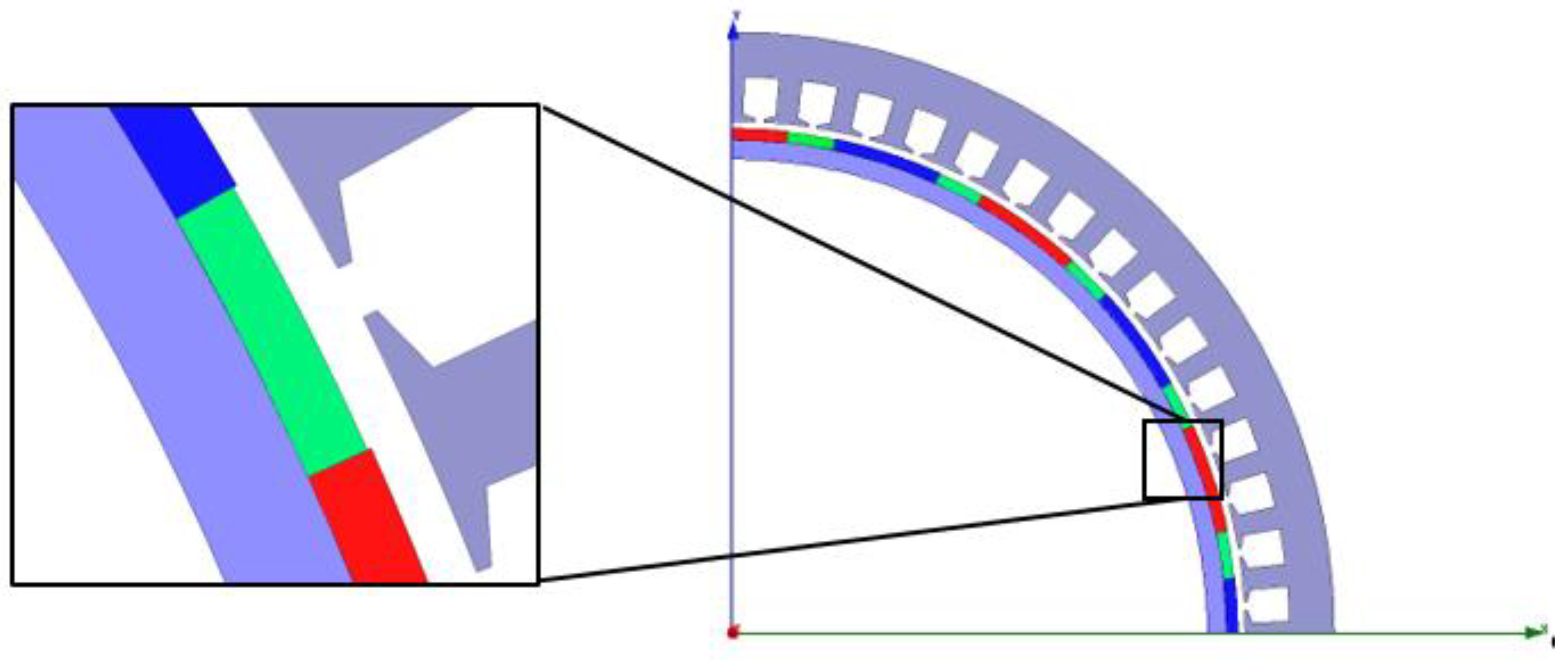
2. Motor Model Description
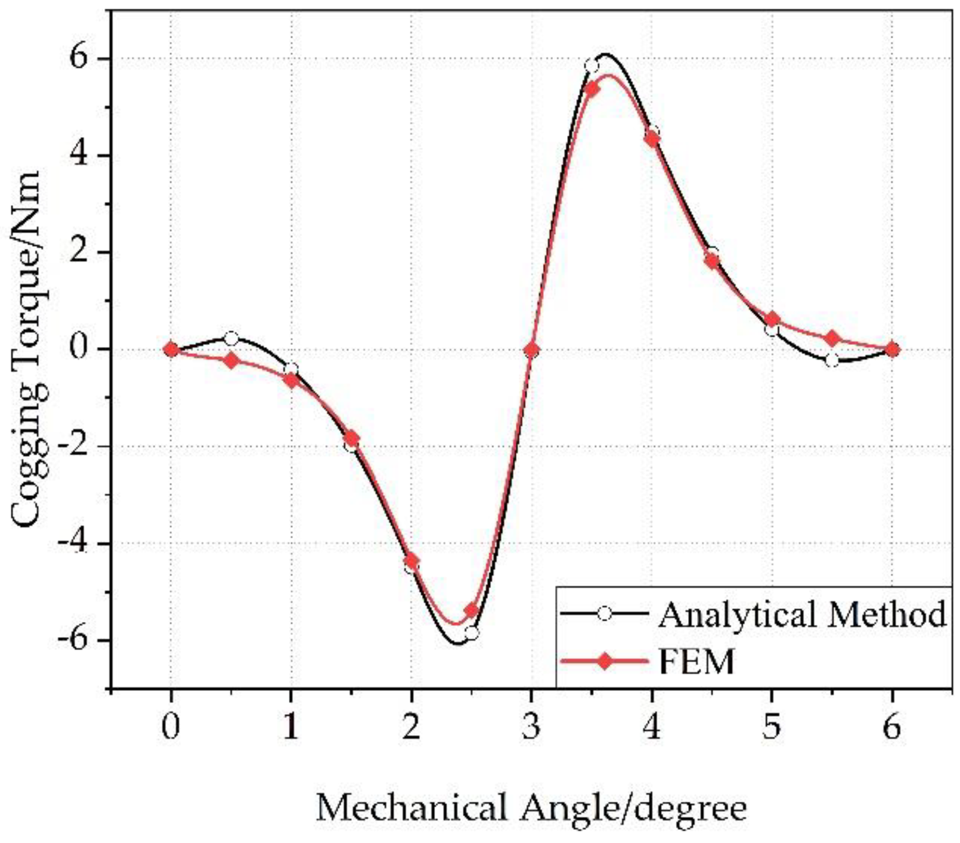
3. Cogging Torque Analysis Model
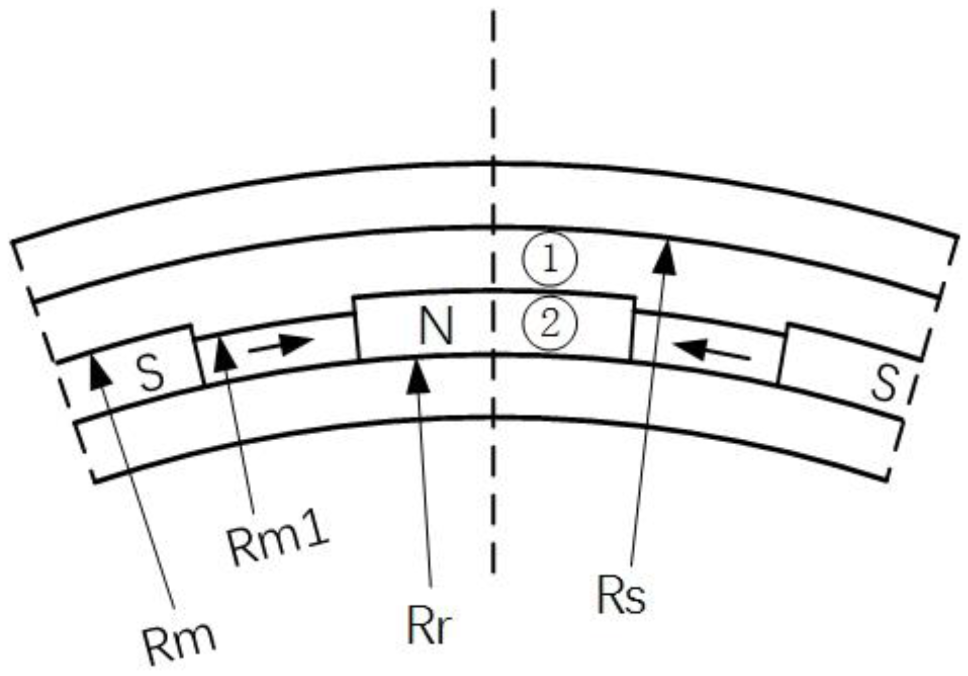
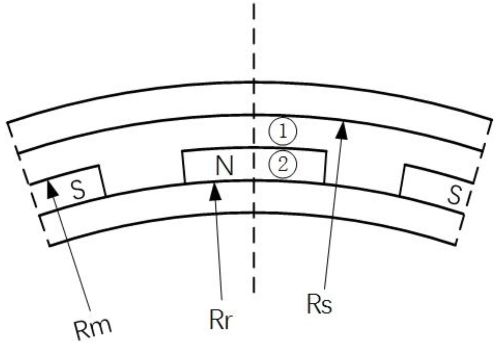
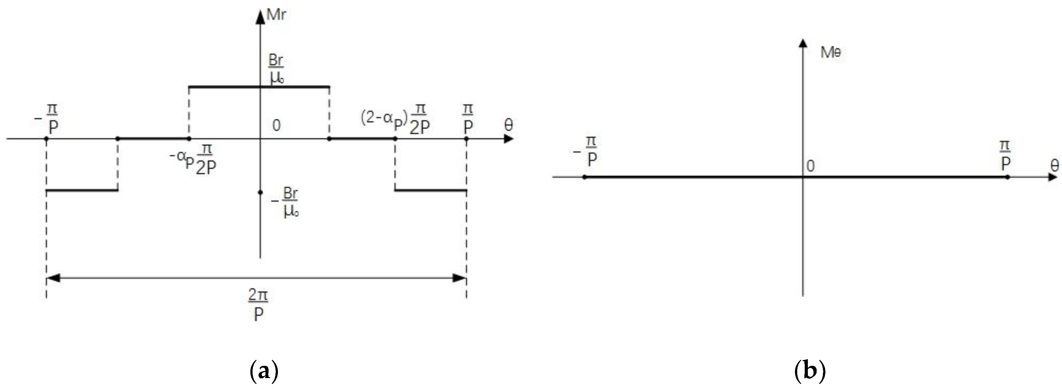
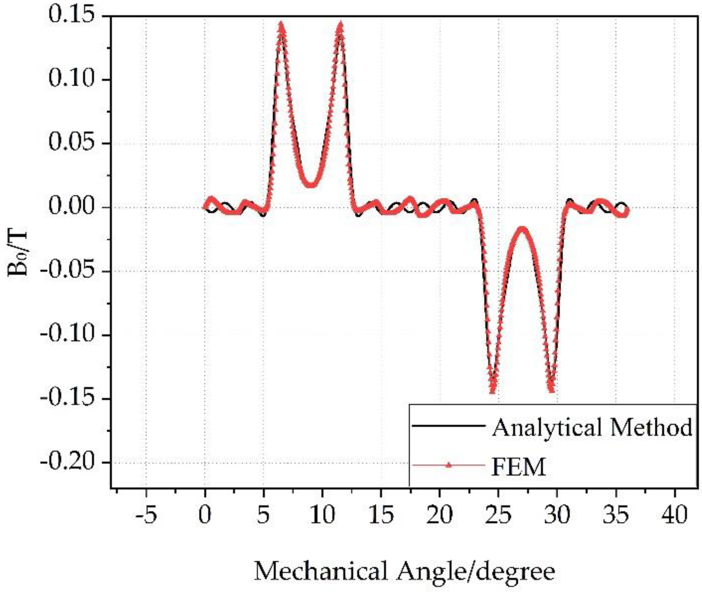
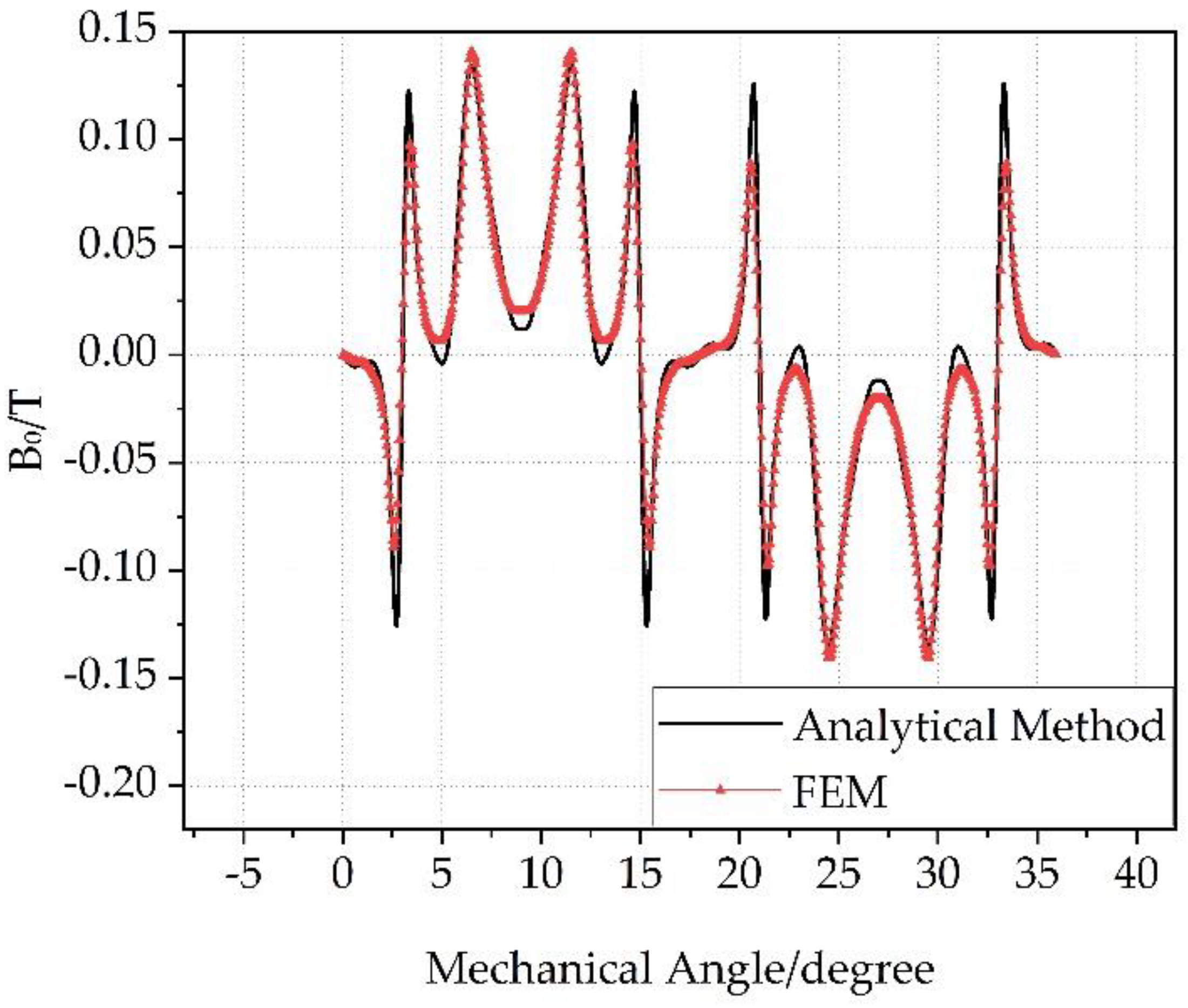
3.1. The Magnetic Field of Slotless Model
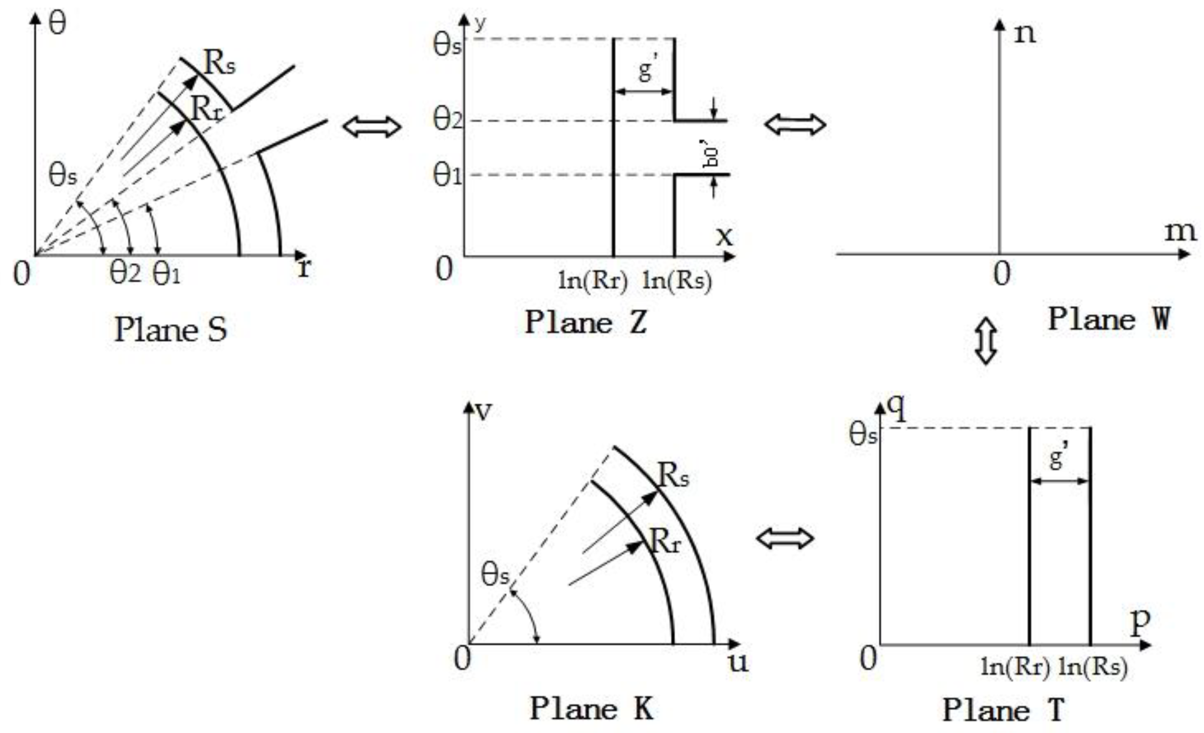
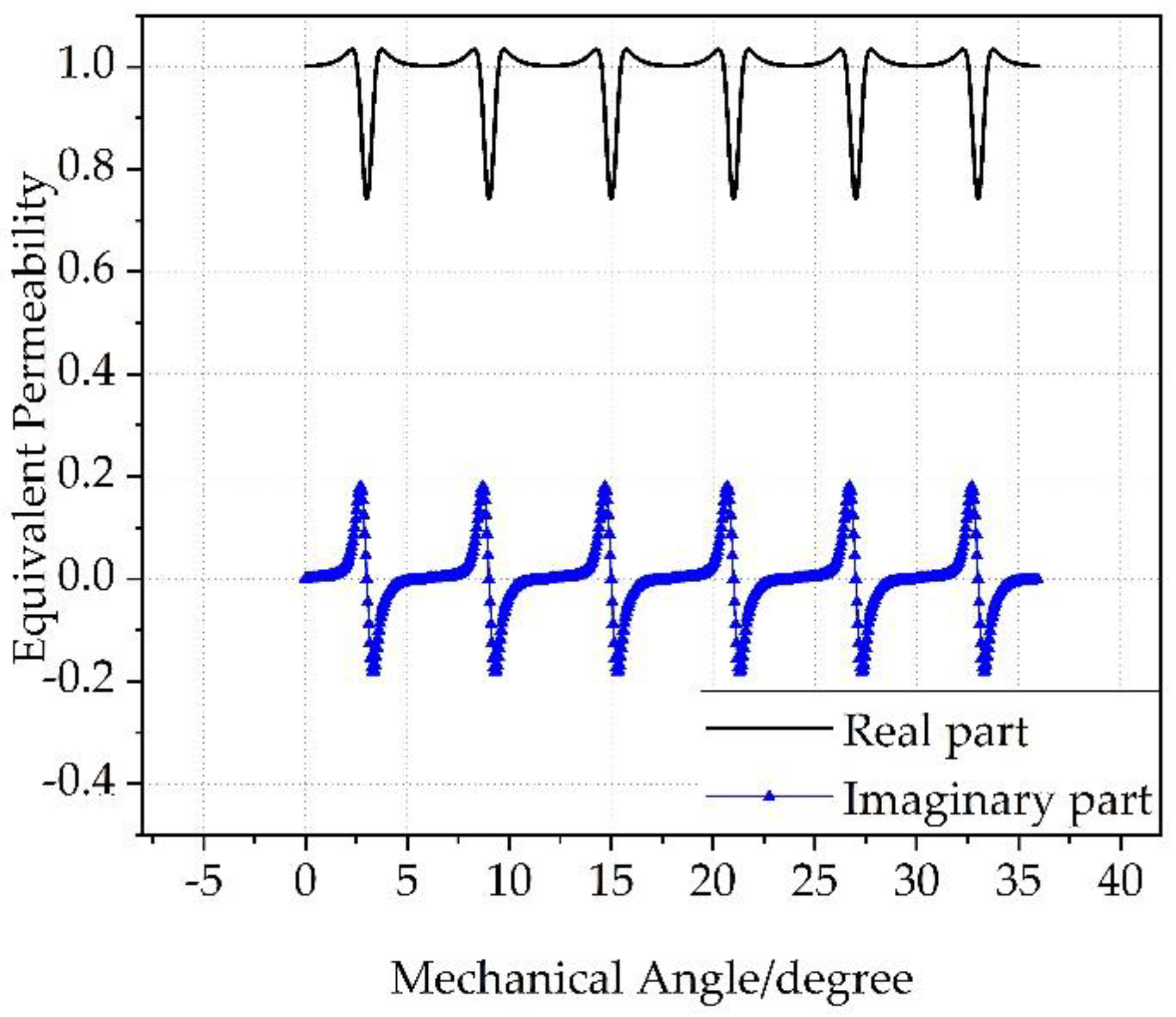
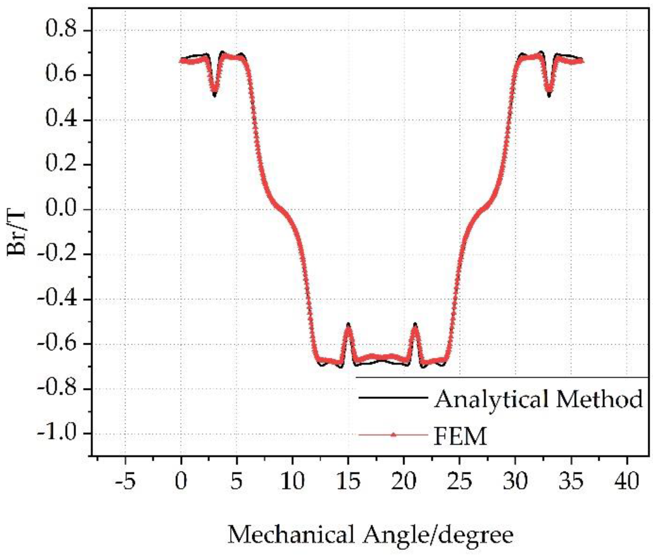
3.2. The Magnetic Field of the Slotted Model
4. Optimization of Halbach Auxiliary Pole Size
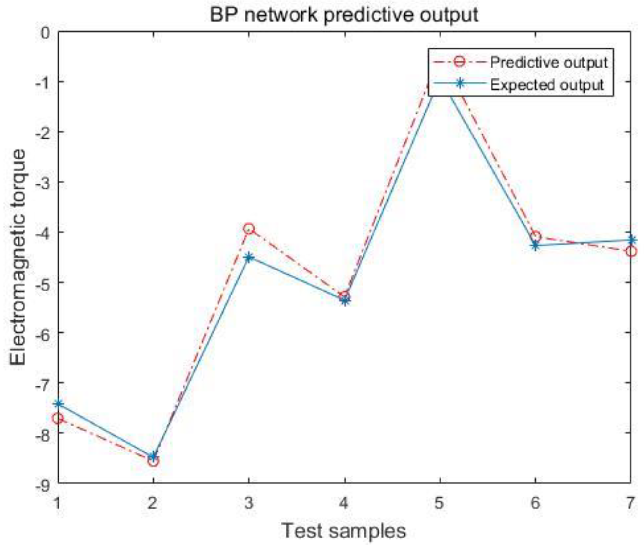
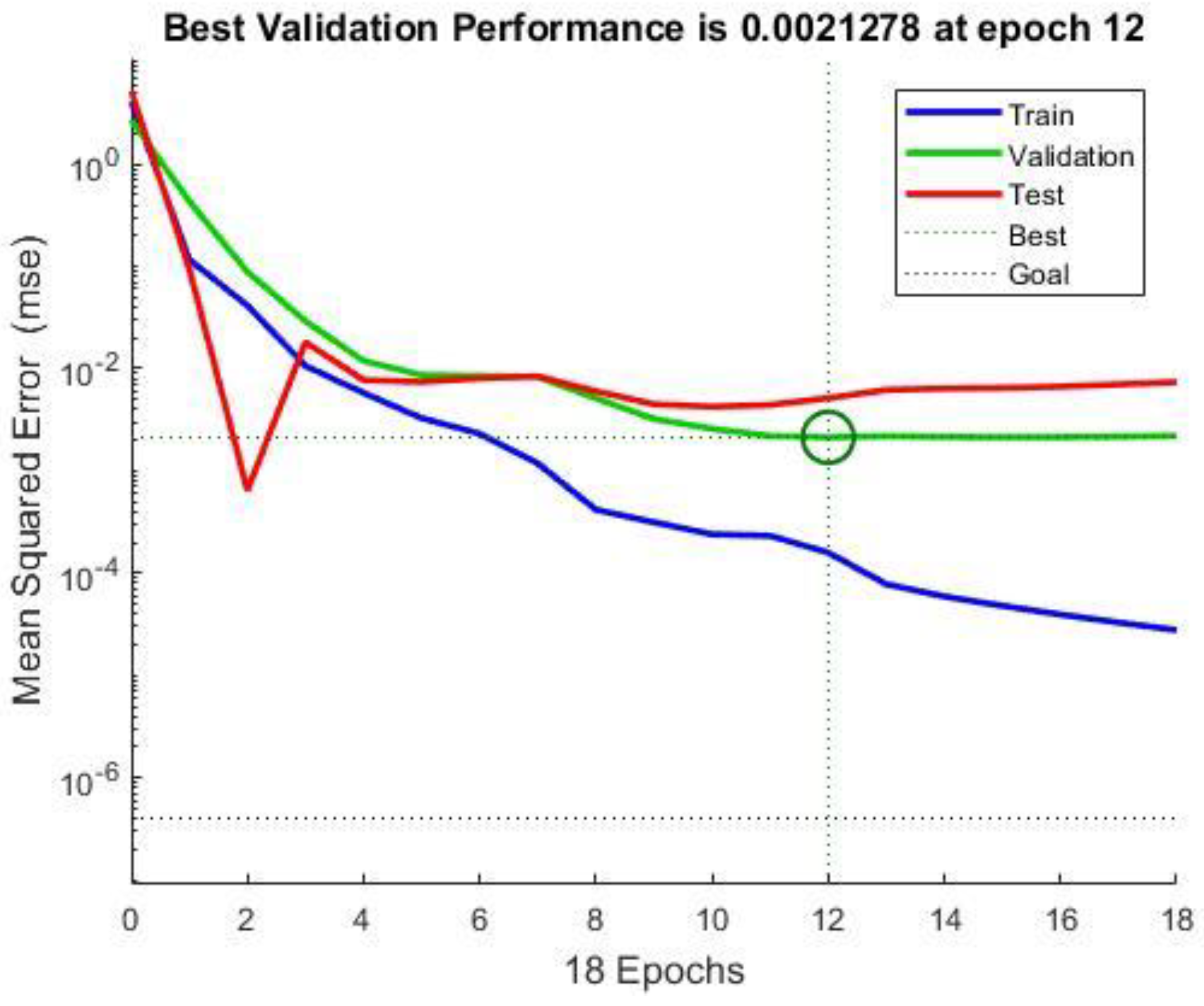
4.1. Calculate Sample Data
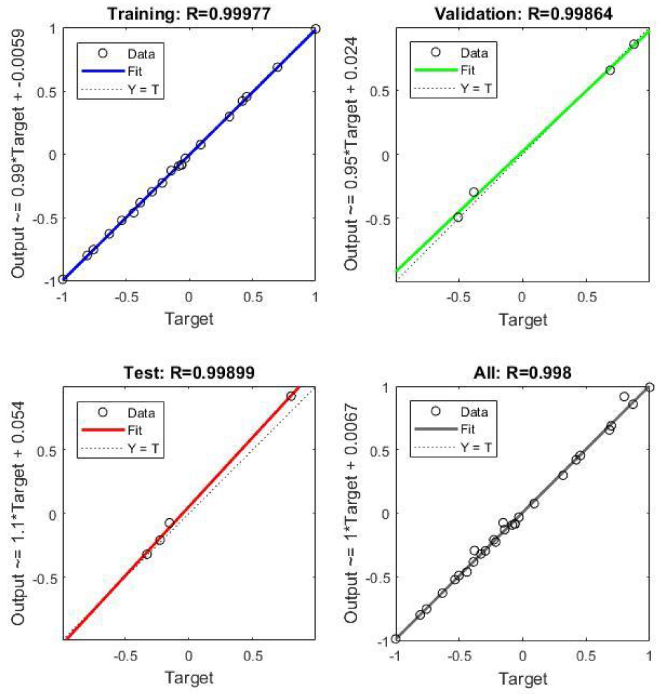
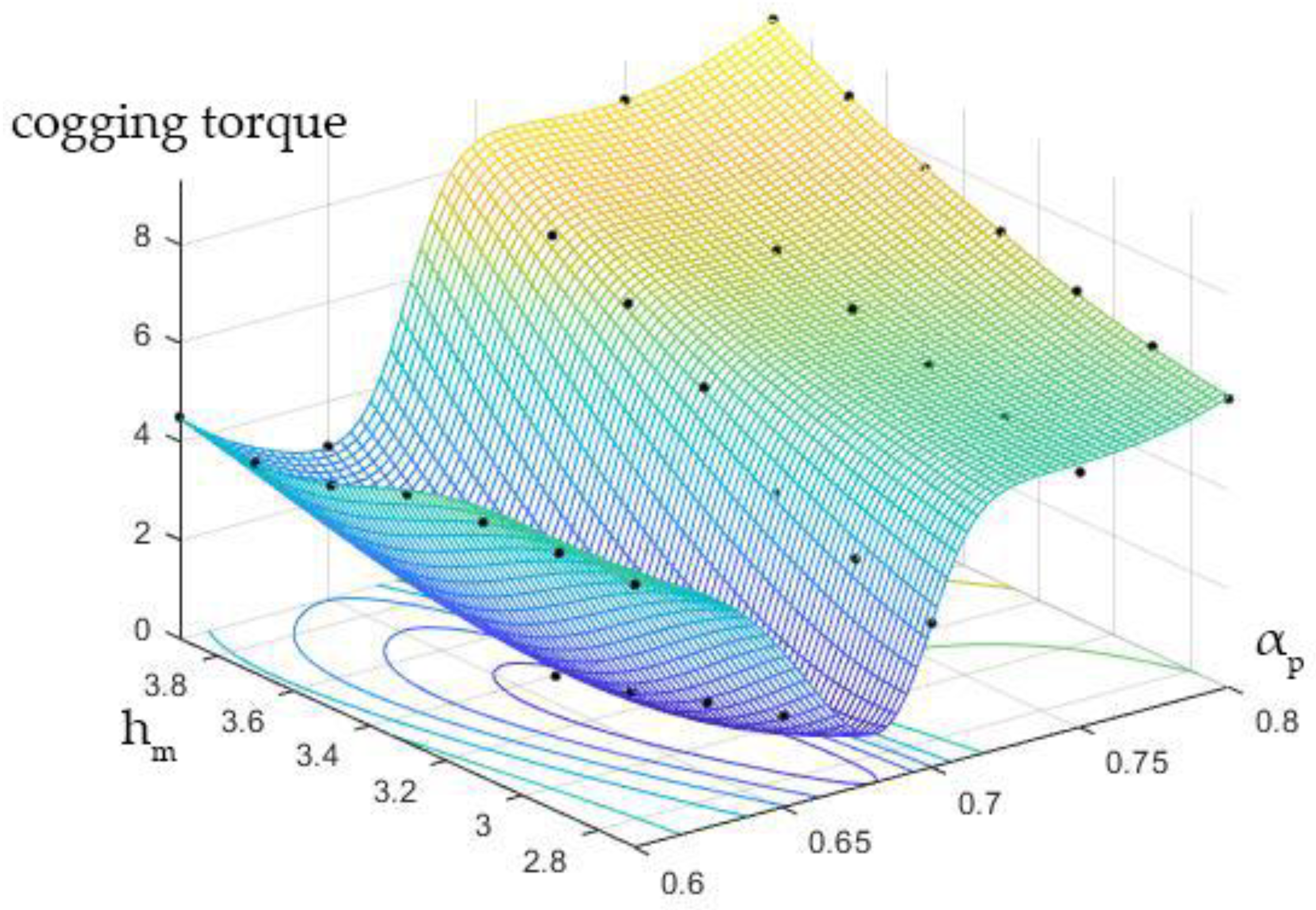
4.2. Size Optimization
5. Conclusions
Author Contributions
Funding
Conflicts of Interest
References
- Li, Y.; Mao, Z.; Song, B.; Tian, W. Design and analysis of stator modular integrated motor propulsor. In Proceedings of the OCEANS 2017, Aberdeen, UK, 19–22 June 2017; pp. 1–6. [Google Scholar]
- Ahn, J.; Park, C.; Choi, S.; Choi, J.; Jang, S. Integrated motor propulsor magnet design with Halbach array for torque ripple reduction. In Proceedings of the 2015 IEEE International Magnetics Conference (INTERMAG), Beijing, China, 11–15 May 2015; p. 1. [Google Scholar]
- Halbach, K. Design of permanent magnet multipole magnets with oriented rare earth cobalt material. Nucl. Instrum. Methods 1980, 169, 1–10. [Google Scholar] [CrossRef]
- Suzuki, H.; Sato, M.; Hanafi, A.I.M.; Itoi, Y.; Suzuki, S.; Ito, A. Magnetic field performance of round layout linear Halbach array using cylinder-shaped permanent magnets. In Proceedings of the 2017 11th International Symposium on Linear Drives for Industry Applications (LDIA), Osaka, Japan, 6–8 September 2017; pp. 1–2. [Google Scholar]
- Li, H.; Xia, C.; Song, P.; Shi, T. Magnetic Field Analysis of a Halbach Array PM Spherical Motor. In Proceedings of the 2007 IEEE International Conference on Automation and Logistics, Jinan, China, 18–21 August 2007; pp. 2019–2023. [Google Scholar]
- Shen, Y.; Hu, P.; Jin, S.; Wei, Y.; Lan, R.; Zhuang, S.; Zhu, H.; Chen, S.; Wang, D.; Liu, D.; et al. Design of Novel Shaftless Pump-Jet Propulsor for Multi-Purpose Long-Range and High-Speed Autonomous Underwater Vehicle. IEEE Trans. Magn. 2016, 52, 1–4. [Google Scholar] [CrossRef]
- Shen, Y.; Zhu, Z.Q. Investigation of permanent magnet brushless machines having unequal-magnet height pole. IEEE Trans. Magn. 2012, 48, 4815–4830. [Google Scholar] [CrossRef]
- Li, Z.; Chen, J.; Zhang, C.; Liu, L.; Wang, X. Cogging torque reduction in external-rotor permanent magnet torque motor based on different shape of magnet. In Proceedings of the 2017 IEEE International Conference on Cybernetics and Intelligent Systems (CIS) and IEEE Conference on Robotics, Automation and Mechatronics (RAM), Ningbo, China, 19–21 November 2017; pp. 304–309. [Google Scholar]
- Jo, I.; Lee, H.; Jeong, G.; Ji, W.; Park, C. A Study on the Reduction of Cogging Torque for the Skew of a Magnetic Geared Synchronous Motor. IEEE Trans. Magn. 2019, 55, 1–5. [Google Scholar] [CrossRef]
- Wang, D.; Wang, X.; Jung, S. Cogging Torque Minimization and Torque Ripple Suppression in Surface-Mounted Permanent Magnet Synchronous Machines Using Different Magnet Widths. IEEE Trans. Magn. 2013, 49, 2295–2298. [Google Scholar] [CrossRef]
- Breton, C.; Bartolome, J.; Benito, J.A.; Tassinario, G.; Flotats, I.; Lu, C.W.; Chalmers, B.J.A. Influence of machine symmetry on reduction of cogging torque in permanent-magnet brushless motors. IEEE Trans. Magn. 2000, 36, 3819–3823. [Google Scholar] [CrossRef]
- Goryca, Z.; Paduszyński, K.; Pakosz, A. Model of the multipolar engine with decreased cogging torque by asymmetrical distribution of the magnets. Open Phys. 2018, 16, 42–45. [Google Scholar] [CrossRef]
- Xia, Z.P.; Zhu, Z.Q.; Howe, D. Analytical magnetic field analysis of Halbach magnetized permanent-magnet machines. IEEE Trans. Magn. 2004, 40, 1864–1872. [Google Scholar] [CrossRef]
- Zhu, Z.Q.; Howe, D.; Chan, C.C. Improved analytical model for predicting the magnetic field distribution in brushless permanent-magnet machines. IEEE Trans. Magn. 2002, 38, 229–238. [Google Scholar] [CrossRef]
- Rabinovici, R. Magnetic field analysis of permanent magnet motors. IEEE Trans. Magn. 1996, 32, 265–269. [Google Scholar] [CrossRef]
- Ma, J.; Tao, R.; Lee, X. Analytical calculation of no-load magnetic field distribution in the slotted airgap of a permanent magnet synchronous motor. In Proceedings of the 6th IFAC Symposium on Mechatronic Systems, Hangzhou, China, 3–5 August 2013; pp. 184–189. [Google Scholar]
- Gu, L.; Wang, S.; Patil, D.; Fahimi, B.; Moallem, M. An improved conformal mapping aided field reconstruction method for modeling of interior permanent magnet synchronous machines. In Proceedings of the 2016 IEEE Energy Conversion Congress and Exposition (ECCE), Milwaukee, WI, USA, 18–22 September 2016; pp. 1–7. [Google Scholar]
- Zhu, L.; Jiang, S.Z.; Zhu, Z.Q.; Chan, C.C. Comparison of alternate analytical models for predicting cogging torque in surface-mounted permanent magnet machines. In Proceedings of the 2008 IEEE Vehicle Power and Propulsion Conference, Harbin, China, 3–5 September 2008; pp. 1–6. [Google Scholar]
- Mao, Z.; Zhao, F. Structure optimization of a vibration suppression device for underwater moored platforms using CFD and neural network. Complexity 2017, 2017, 5392539. [Google Scholar] [CrossRef]
- Liang, C.J.; Yang, G.L.; Wang, X.F. Structural Dynamics Optimization of Gun Based on Neural Networks and Genetic Algorithms. J. Ordnance Ind. 2015, 36, 789–794. [Google Scholar]


| Structural Parameters | Value | Structural Parameters | Value |
|---|---|---|---|
| Number of pole pairs | 10 | Stator tooth height (mm) | 14 |
| Number of slots | 60 | Rotor outer diameter (mm) | 319 |
| OD of stator (mm) | 380 | Rotor yoke thickness (mm) | 6 |
| ID of stator (mm) | 324 | Main pole thickness (mm) | 3.5 |
| Notch width (mm) | 2.8 | Pole embrace | 0.7 |
| Stator tooth width (mm) | 6.6 |
| Cogging Torque (Nm) | Radial Thickness of Auxiliary Pole (mm) | |||||||
|---|---|---|---|---|---|---|---|---|
| 2.7 | 2.9 | 3.1 | 3.3 | 3.5 | 3.7 | 3.9 | ||
| Pole Embrace | 0.60 | 5.354 | 5.281 | 5.196 | 5.054 | 4.527 | 4.268 | 4.493 |
| 0.65 | 1.867 | 1.424 | 0.945 | 0.546 | 1.122 | 1.932 | 3.080 | |
| 0.70 | 2.936 | 3.531 | 4.156 | 5.593 | 6.585 | 7.258 | 8.236 | |
| 0.75 | 5.182 | 5.545 | 5.917 | 6.366 | 6.842 | 7.412 | 8.475 | |
| 0.80 | 5.852 | 6.210 | 6.620 | 7.120 | 7.689 | 8.450 | 9.297 | |
| Comparison Items | The Reduction Percentages |
|---|---|
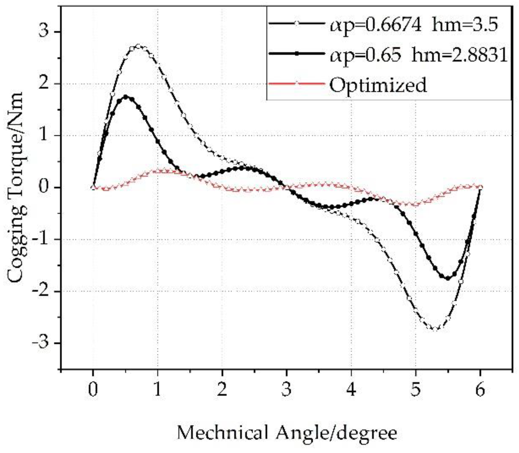
| Cogging Torque | 88% |
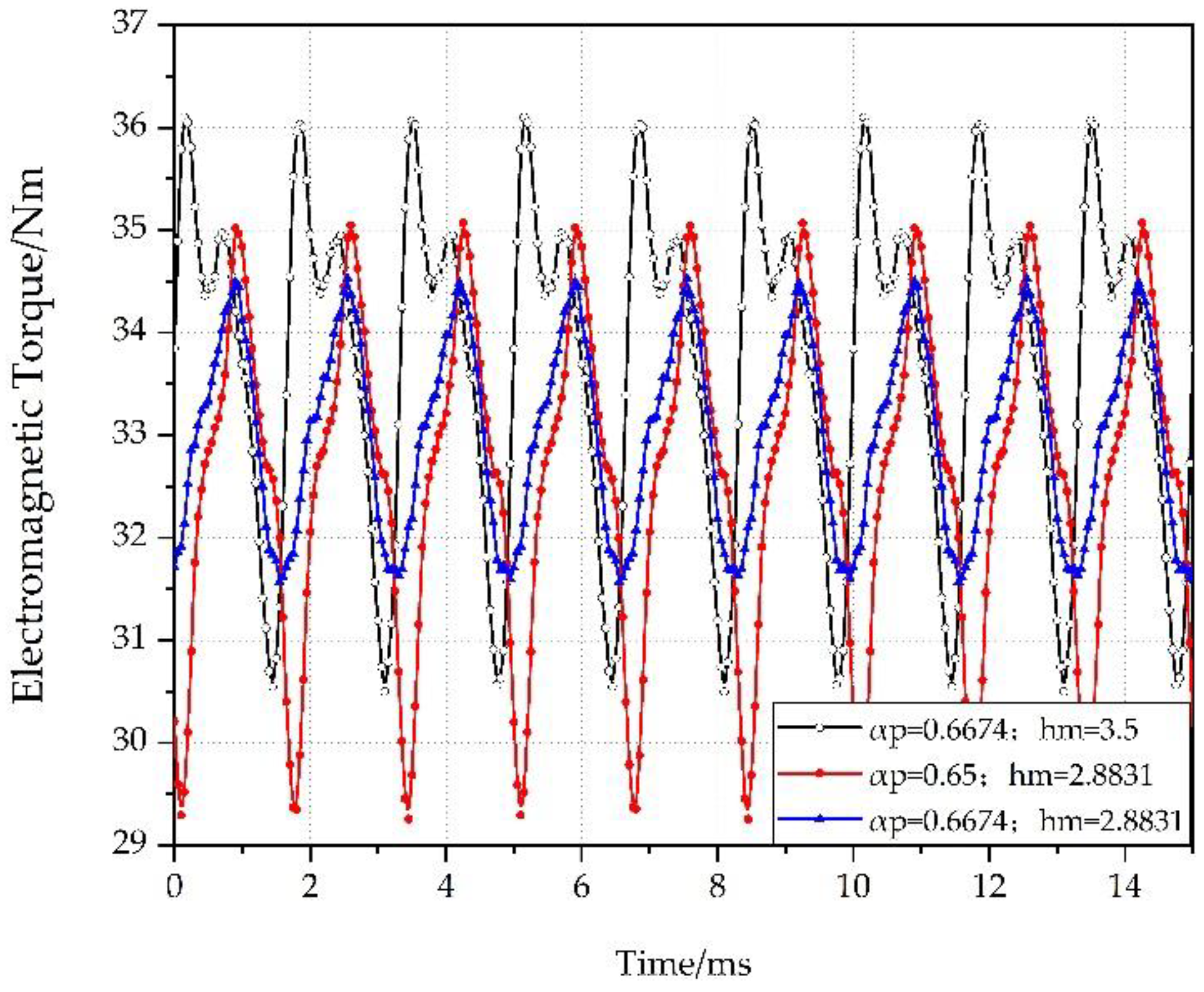
| Torque Ripple | 45% |
| Average Electromagnetic Torque | Not changes |
© 2019 by the authors. Licensee MDPI, Basel, Switzerland. This article is an open access article distributed under the terms and conditions of the Creative Commons Attribution (CC BY) license (http://creativecommons.org/licenses/by/4.0/).
Share and Cite
Ou, H.; Hu, Y.; Mao, Z.; Li, Y. A Method for Reducing Cogging Torque of Integrated Propulsion Motor. J. Mar. Sci. Eng. 2019, 7, 236. https://doi.org/10.3390/jmse7070236
Ou H, Hu Y, Mao Z, Li Y. A Method for Reducing Cogging Torque of Integrated Propulsion Motor. Journal of Marine Science and Engineering. 2019; 7(7):236. https://doi.org/10.3390/jmse7070236
Chicago/Turabian StyleOu, Huanyu, Yuli Hu, Zhaoyong Mao, and Yukai Li. 2019. "A Method for Reducing Cogging Torque of Integrated Propulsion Motor" Journal of Marine Science and Engineering 7, no. 7: 236. https://doi.org/10.3390/jmse7070236
APA StyleOu, H., Hu, Y., Mao, Z., & Li, Y. (2019). A Method for Reducing Cogging Torque of Integrated Propulsion Motor. Journal of Marine Science and Engineering, 7(7), 236. https://doi.org/10.3390/jmse7070236