Research on a Method for Simulating Multiview Ocean Wave Synchronization Data by Networked SAR Satellites

Abstract

It is expected that the problem of the azimuth cutoff wavelength in single-satellite synthetic aperture radar (SAR) observations can be solved by means of the cooperative observation of networked SAR satellites. Multiview SAR wave synchronization data are required in the process. However, most of the current orbiting satellites are geosynchronous orbit satellites; the simultaneous observation by multiple SARs in the same sea area cannot be achieved, and multiview synchronization data cannot be obtained. Therefore, this paper studies the simulation of the multiview SAR wave synchronization data. Ocean wave spectra were simulated by using the Pierson Moskowitz (PM) spectrum. The Monte Carlo method was used to simulate two-dimensional (2D) ocean surfaces at different wind speeds. The two-scale electromagnetic scattering model was used to calculate the ocean surface backscattering coefficient, and the time-domain echo algorithm was used to generate echo signals. The echo signals were processed by the Range–Doppler (RD) imaging algorithm to obtain ocean SAR data. Based on the obtained single-SAR wave data, networked satellites consisting of three SARs were simulated, and the SAR wave data were synchronized. The results show that when SARs are used to observe the same sea area from different observation directions, the clarity of the wave fringes in the SAR images are different. For different azimuth angles, the degrees of azimuth cutoff are different. These results reflect the influences of different degrees of azimuth cutoff on SAR images. The simulated wave synchronization data can be used as the basic data source for subsequent azimuth cutoff wavelength compensation.

1. Introduction

Ocean waves are small-scale wind-gravity waves that occur on ocean surfaces, including sea and swell, and are also an important ocean dynamic process. For many situations, it is necessary to understand their internal structures, such as marine transportation, offshore platforms, and ocean wave parameters at specific locations for ports and ocean engineering [1].

The common methods for obtaining ocean wave information include numerical models, field observations, and remote sensing observations. A numerical model uses mainly mathematical operations to calculate and predict the sea state. Although the model can obtain the results of ocean wave parameters of long-term sequences, it is affected by multiple conditions, such as initial condition settings, observation data assimilation and water depth. Field observations mainly consist of sea state measurements from buoys [2]. Buoys are recognized as more accurate means in the field observation of ocean waves; however, buoy locations are sparse, and the data records at each position may be discontinuous [3]. Buoys can verify the ocean wave parameters obtained by numerical models and remote sensing [4]. Remote sensing obtains the sea state by means of a synthetic aperture radar (SAR), altimetry and scatterometry. Altimeters and scatterometers are highly susceptible to the underwater terrain when observing waves. Although altimeters provide uniform, repetitive measurements of the significant wave height (SWH), other wave parameters, such as the mean wave period, cannot be observed by altimeters [5,6]. Scatterometers are most prominent for the observation of surface winds over global oceans instead of ocean waves [7]. Compared with numerical models and in situ buoy measurements at a single location, SARs are effective and of great interest because of the high spatial resolution and the almost instantaneous observation potential of large ocean areas [8]. As a powerful instrument to measure ocean waves, a SAR can work all day under almost any weather condition [9]. A SAR has multiband and multipolarization characteristics, which allow the estimation of the spatial distributions of the investigated characteristics [10]. Especially important, the ocean observation results provided by SARs are not affected by the underwater terrain. Therefore, this paper intends to use SARs to achieve the observation of ocean waves.

However, it is known that SAR images of oceanic scenes include velocity bunching caused by the orbital motions of ocean waves. Velocity bunching leads to a nonlinear imaging mechanism in ocean SAR images [11]. Accordingly, ocean SAR images become blurred, especially in the azimuth direction (the direction parallel to the SAR flight direction is the azimuth direction, and the SAR look direction is defined as the range direction) [12]. This phenomenon is known as the azimuth cutoff wavelength or simply the azimuth cutoff, and affects only the azimuthally traveling waves [13]. This phenomenon leads to information on SAR observations that mainly contains low-wavenumber swell, and only waves with a wavelength greater than the azimuth cutoff wavelength can be observed [14]. This condition is a fatal flaw in the observation of ocean waves by a single SAR satellite, which greatly limits the observation capability and integrity of SAR.

The azimuth cutoff wavelength is an inherent drawback of SAR and has not received much attention as a helpful sea state parameter. In 1996, Kerbaol V et al. proposed evidence of the azimuth cutoff dependency on the wind speed and SWH [15]. In 2014, Ren et al. proposed two models to directly retrieve the SWH uWHW Wsing the azimuth cutoff [16]. In 2015, Justin E. Stopa et al. estimated the wave orbital velocity from the azimuth cutoff wavelength using Envisat advanced synthetic aperture radar (ASAR) measurements [17]. Most of the above studies focus on the mutual estimation of the azimuth cutoff wavelength and parameters such as the SWH and wind speed. Currently, there is no research on compensating the azimuth cutoff wavelength, which is the subject of this paper. The premise of this study is that networked satellites are needed to coordinate observations to obtain multidirectional SAR wave synchronization data. This requirement is because the azimuth cutoff degrees caused by different SAR observation directions are different, and the synchronization data with different cutoff degrees can be combined by weight to effectively compensate for the impact of the azimuth cutoff.

At present, most satellites in orbit are geosynchronous orbit satellites. There is no angle between the orbits of the satellites. The simultaneous observation of multiple SARs in the same sea area cannot be achieved, and multiview synchronization data cannot be obtained. Therefore, it is necessary to acquire multiview synchronization data by means of SAR imaging simulations and carry out preresearch work on multiple SAR observation waves, which lays the foundation for future observations of networked SAR satellites. In general, ocean SAR imaging simulations can be separated into two methods. For the first method, ocean SAR data are simulated at the image level: By using certain equations, SAR imagery is numerically computed [18]. In 2009, Zhao et al. analyzed the influences of ocean wave parameters on SAR images and obtained ocean surface polarized SAR images [19]. In 2011, Guo et al. simulated polarized ocean SAR images based on a random sea surface model and an electromagnetic scattering model [20]. Although this method avoids the calculation of complex raw SAR data, the method cannot comprehensively reflect the characteristics of the SAR system. The second method is to indirectly obtain ocean SAR images by simulating raw SAR echo signals. In 1998, G. Franceschetti et al. used the coordinate transformation method to obtain ocean scene SAR echoes [21]. In 2012, Zhu et al. studied the imaging simulation of ocean surfaces by missile-borne SARs in side-looking and squint modes [22]. In 2018, Fan et al. studied the SAR imaging simulation of composite scenes in the squint mode [23]. The imaging method used in this paper is the second method, which has the advantages of not relying on the imaging model and high precision of the imaging results compared with the first method.

However, most of the current studies are single-SAR imaging simulations, and the imaging simulation of multiple SARs has not been studied. In this paper, the imaging simulation of a network of satellites consisting of three SAR satellites was carried out on the basis of single-SAR imaging simulations. The main work of this paper is as follows: Aimed at the problem of the azimuth cutoff for ocean waves observed by a single SAR satellite, a network of SAR satellites with three SARs was simulated, and then, multiview SAR ocean wave synchronization data were simulated.

The structure of this paper is as follows: In Section 2, the basic principles of single-SAR imaging simulation are introduced. In Section 3, the results of the imaging simulations are analyzed and then the simulation of networked SAR satellites is described. Section 4 presents a discussion. Conclusions are provided in the final section.

2. Basic Principle of SAR Imaging Simulation

The flow of imaging simulation in this paper is composed of wave spectrum simulation, sea surface simulation, SAR echo signal simulation, sea surface SAR imaging, etc.

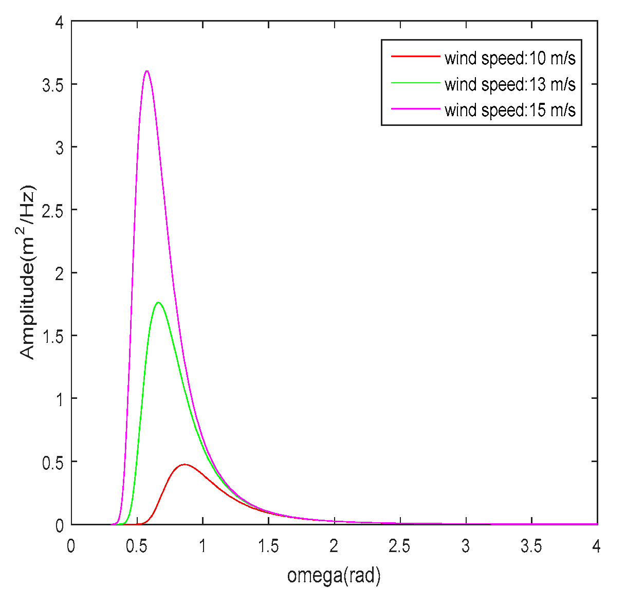
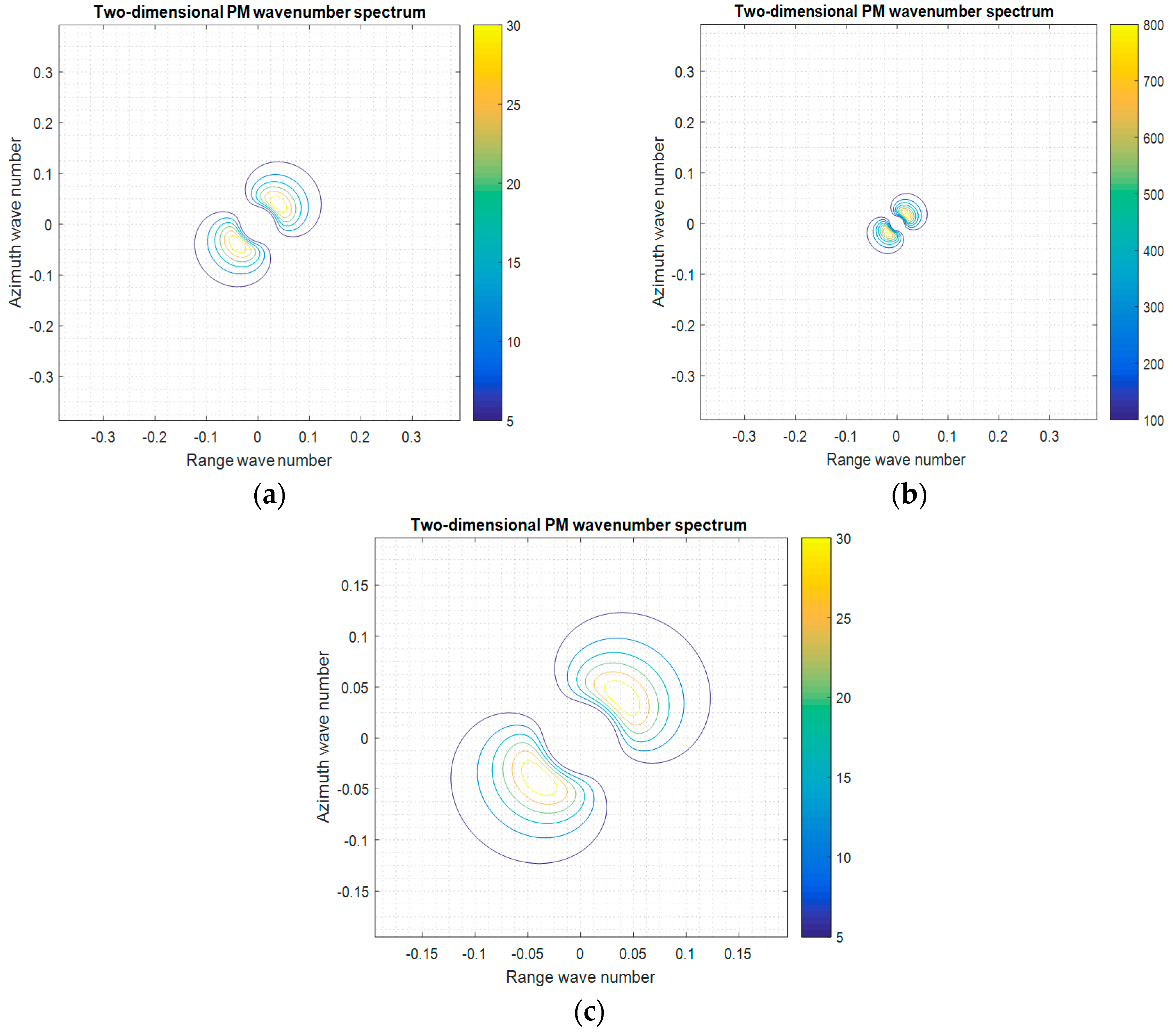
2.1. Wave Spectrum Simulation

In this paper, the Pierson Moskowitz (PM) spectrum was used to complete the wave spectrum simulations. The PM spectrum belongs to the gravity spectra and is also a kind of steady-state sea spectrum. The one-dimensional (1-D) PM wave spectrum model is as follows:

$$S(\omega )=\frac{\mathrm{a}{g}^2}{{\omega }^5}\exp [-b{(\frac{g}{U_{19.5}\omega })}^4]$$

(1)

where a = 0.0081, b = 0.74, g is the acceleration due to gravity, $U_{19.5}$ represents the wind speed at a height of 19.5 m above the sea surface, $\mathsf{\omega }$ is the frequency and $\mathrm{S}\left(\mathsf{\omega }\right)$ is the value of the PM spectrum. However, in the calculation of ocean waves, the wind speed at a height of 10 m ($U_{10}$) above the sea surface is usually selected, and the conversion relationship between the wind speeds [24] is as follows:

$$U_h=U_{10}·(1+2.5{\log }_{10}^{0.1*h}(\sqrt{0.0015/[1+\exp \left(-\frac{U_{10}-1.25}{1.56}\right)}]+0.00104))$$

(2)

where h is the sea surface height and $U_h$ represents the wind speed at different sea surface heights, except 10 m.

It is necessary to describe the waves in the different propagation directions by means of a direction function. The 1D wave spectrum is multiplied by the normalized direction function to obtain the two-dimensional (2D) wave direction spectrum. The direction function selected in this paper is as follows:

$$G_{PM}(\varphi )=\frac{2}{\pi }{\cos }^2(\frac{\varphi -{\varphi }_m}{2})$$

(3)

where $\varphi$ denotes the wave propagation direction, ${\varphi }_m$ is the wave direction of the main wave, usually taken as the wind direction angle, so $\varphi -{\varphi }_m$ represents the angle between $\varphi$ and ${\varphi }_m$, which is usually called the azimuth angle. According to the relationship to gravity dispersion, the 2D wave direction spectrum is converted into a 2D wavenumber direction spectrum, and the expression is as follows:

$${\mathrm{S}}_{PM}(\mathrm{K},\varphi )=\frac{a}{2K^4}\exp (-\frac{b{g}^2}{K^2{U}_{19.5}^4})·\frac{2}{\pi }{\cos }^2(\frac{\varphi -{\varphi }_m}{2})$$

(4)

In the equation, the values of a, b, and g are the same as those in Equation (1), K denotes the wavenumber, and $S_{PM}\left(K,\varphi \right)$ represents the wavenumber direction spectrum.

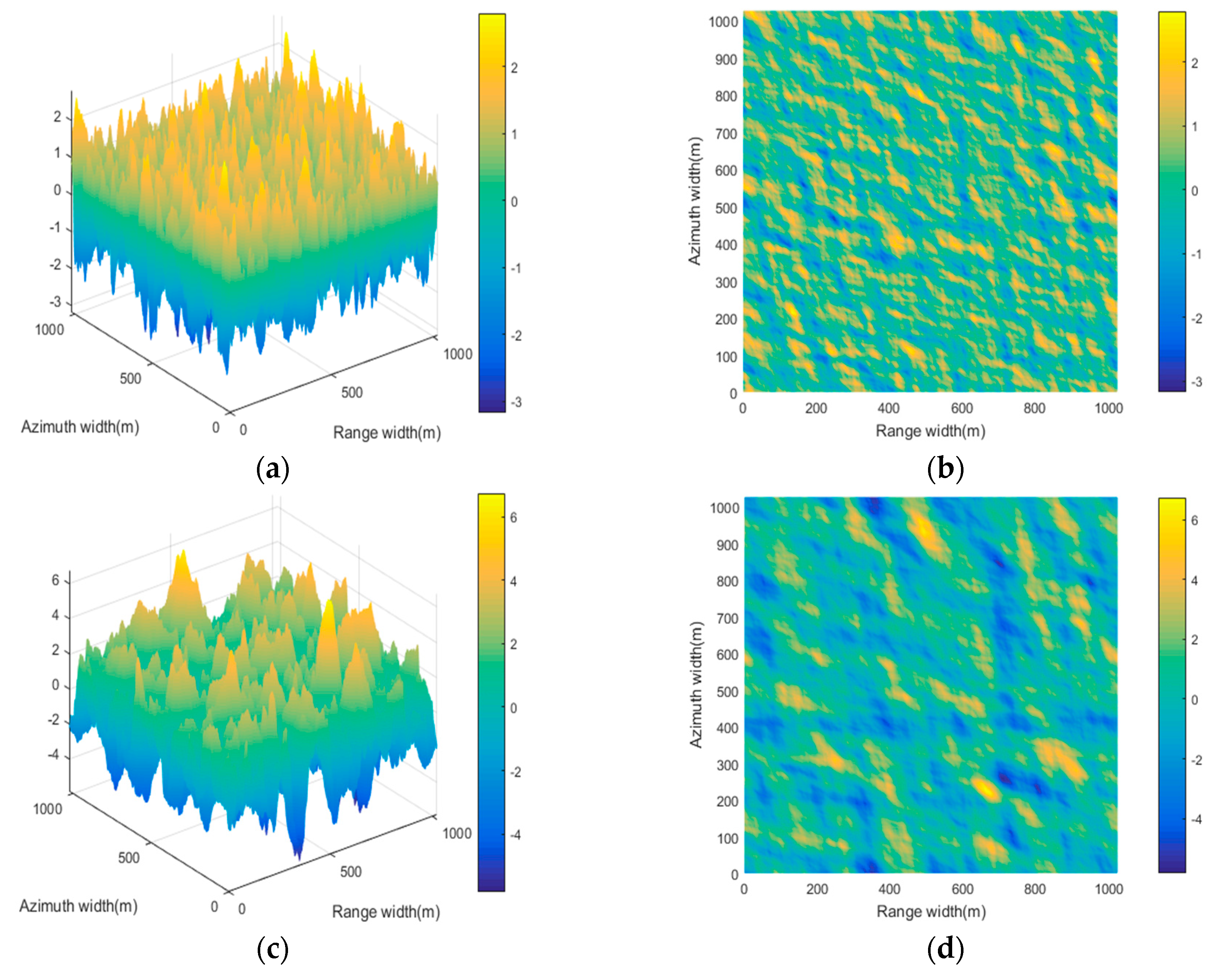
2.2. Ocean Surface Simulation

The accuracy of the constructed ocean surface directly determines the accuracy of the ocean surface backscatter coefficient. In this paper, the Monte Carlo method was used to complete the simulation of the 2D ocean surface. The fast Fourier transform (FFT) expression equation of the ocean surface height fluctuation function is as follows [25]:

$$\begin{array}{ll}F\left(k_{m_k},k_{n_k}\right)=& 2\pi {\left[L_x{L}_{y}S\left(k_{m_k},k_{n_k}\right)\right]}^{1/2}\\ & \times \{\begin{array}{ll}\frac{\left[N\left(0,1\right)+iN\left(0,1\right)\right]}{\sqrt{2}},& m_k\ne 0,M/2\mathrm{and}{n}_k\ne 0,N/2\\ N\left(0,1\right),& m_k=0,M/2\mathrm{or}{n}_k=0,N/2\end{array}\end{array}$$

(5)

where $L_x\mathrm{and} L_y$ represent the length of the 2D ocean surface in the range direction and azimuth direction, respectively; M and N represent the sampling points of the ocean surface in the range and azimuth directions, respectively; $m_k \mathrm{and} n_k$ represent the range of the sampling points; $\mathrm{S}\left(k_{m_k},k_{n_k}\right)$ is the 2D PM wavenumber spectrum; $k_{m_k}=2\pi m_k/L_x \mathrm{and}{k}_{n_k}=2\pi n_k/L_y$ are the range and azimuth wavenumbers, respectively; and N(0, 1) represents a random number obeying a Gaussian distribution with a mean of 0 and a variance of 1. By performing the inverse Fourier transform (IFFT), the sea surface height fluctuation function $\mathrm{f}\left(x_m,y_n\right)$ can be simulated. The expression equation is as follows [25]:

$$f\left(x_m,y_n\right)=\frac{1}{L_x{L}_y}{\displaystyle \sum _{m_k=-M/2+1}^{M/2}{\displaystyle \sum _{n_k=-N/2+1}^{N/2}F\left(k_{m_k},k_{n_k}\right)\exp \left[i\left(k_{m_k}{x}_m+k_{n_k}{y}_n\right)\right]}}$$

(6)

where $\left(x_m,y_n\right)$ indicates the coordinates of the sea surface and the other variables have the same meaning as in Equation (5).

2.3. SAR Echo Signal Simulation

In the process of ocean surface echo signal simulation, there are two key problems to be solved. One problem is the calculation of the ocean surface backscattering coefficient, and the other problem is the generation of echo signals. Among these problems, the calculation of the backscattering coefficient is the basis of the echo signals.

2.3.1. Generation of the Ocean Surface Backscattering Coefficient

In this paper, a two-scale electromagnetic scattering model was used to calculate the ocean surface backscattering coefficient, and the SAR working mode was defined as vertical (VV) polarization. The backscattering coefficient under VV polarization can be expressed as follows [26]:

$${\sigma }_{VV}^0({\theta }_i)=\frac{1}{MN}{\sigma }_{BVV}^0({\theta }^{\prime })\frac{{[\sin {\theta }_i-\alpha (x,y)\cos {\theta }_i]}^4[1+\alpha (x,y)\tan {\theta }_i]}{{\{\beta {(x,y)}^2+{[\sin {\theta }_i-\alpha (x,y)\cos {\theta }_i]}^2\}}^2}$$

(7)

where $\mathsf{\alpha }\left(\mathrm{x},\mathrm{y}\right)\mathrm{and}\mathsf{\beta }\left(\mathrm{x},\mathrm{y}\right)$ represent the slopes of the ocean surface at point (x, y), which can be obtained by differentiating, and ${\mathsf{\sigma }}_{BVV}^0\left({\theta }^{\prime }\right)$ is the backscatter coefficient obtained by the perturbation method in the local coordinate system [27] as follows:

$$\begin{array}{l}{\sigma }_{BVV}^0({\theta }_i^{\prime })=8k^4{\cos }^4{\theta }_i^{\prime }|{\mathrm{U}}_{VV}{|}^{2}S(2\mathrm{ksin}{\theta }_i^{\prime },0)\\ {\mathrm{U}}_{VV}=\frac{(\epsilon -1)[\sin {\theta }_i^{\prime }{}^2-\epsilon (1+\sin {\theta }_i^{\prime }{}^2)]}{{[\epsilon \cos {\theta }_i^{\prime }+\sqrt{\epsilon -\sin {\theta }_i^{\prime }{}^2}]}^2}\end{array}$$

(8)

where $\mathsf{\epsilon }$ represents the dielectric constant of seawater and can be obtained by the Debye Equation [28] as follows:

$$\epsilon ={\epsilon }_0+\frac{{\epsilon }_s-{\epsilon }_{\infty }}{1+j\omega \tau }-j\frac{\sigma }{\omega {\epsilon }_0}$$

(9)

where ${\mathsf{\epsilon }}_{\infty }$ represents the dielectric constant of seawater when the frequency is infinite; ${\mathsf{\epsilon }}_s$ denotes the static dielectric constant; $\mathsf{\tau }$ represents the relaxation time; $\mathsf{\sigma }$ is the conductivity of seawater; ${\epsilon }_0=8.854\ast {10}^{-12} F/m$ is the free space permittivity; and the above parameters are all related to the seawater temperature or salinity function [29].

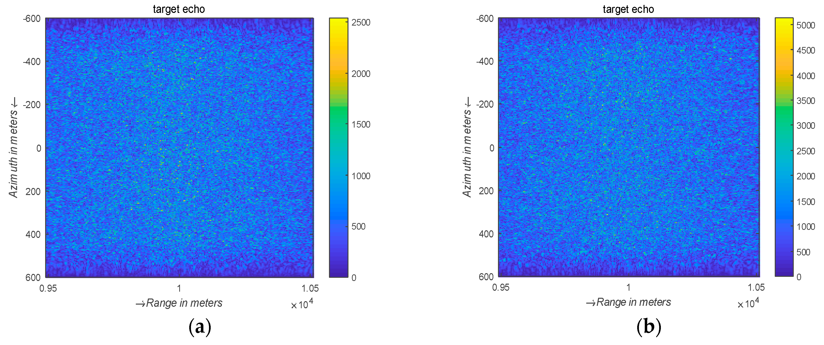
2.3.2. Calculation of the Ocean Surface Echo Signals

The algorithm for simulating echo signals is divided into a time-domain algorithm and frequency-domain algorithm. Among these algorithms, the calculation of the frequency-domain algorithm is relatively small, but the velocity bunching effect cannot be introduced in the process of generating echo signals. The time-domain algorithm simulates the real working process of the SAR receiver and can acquire the original echo signals. Although the calculation amount is large, the generated ocean surface echo signals are the most accurate. Based on the comparison, this paper selected the time-domain algorithm and assumed that the SAR working mode was side-looking to simulate the ocean surface echo signals.

Combined with the SAR operating parameter set in the simulation process, according to the SAR working principle, the 1D echo signal is written in the 2D form with respect to the azimuth and range. After the carrier is removed by quadrature demodulation, the echo of the single-point target can be written as follows [30]:

$$\begin{array}{ll}{s}_r(s,t;r)=& \sigma \cdot rect(\frac{t-2R(s;r)/C}{Tr})\exp [j\pi K_r{(t-2R(s;r)/C)}^2]\cdot \\ & rect(\frac{s}{Tsar})\exp [-j\frac{4\pi }{\lambda }R(s;r)]\end{array}$$

(10)

where PRF is the pulse repetition time, rect represents a rectangular function, C is the speed of light, and σ is the backscattering cross-section of the point target. The echoes of K ideal point targets can be obtained by superposition, as shown in the following Equation [30]:

$$\begin{array}{ll}Sr(n,m)=& {\displaystyle \sum _{k=1}^K\sigma \cdot \exp \{j\pi [t(m)-\frac{2R(n;k)}{C}]\}}\cdot \exp [-j\frac{4\pi }{\lambda }R(n;k)]\\ & 0<[t(m)-\frac{2R(n;k)}{C}]<Tr;|R(n;k)-x(k)|<Tsar\\ & \hfill n=1,2,3\cdots N;m=1,2,3\cdots M\end{array}$$

(11)

where R(n; k) is the slant distance between the SAR and imaging points, Tsar is the SAR integration time, and Tr is the pulse duration. The idea of generating ocean surface echo signals was to calculate the echo signals of all of the points that make up the ocean surface separately and superimpose the echo signals of the points to obtain the echo signals of the whole ocean surface at a certain azimuth, traverse all of the azimuth moments, and finally obtain the echo signals of the entire ocean surface.

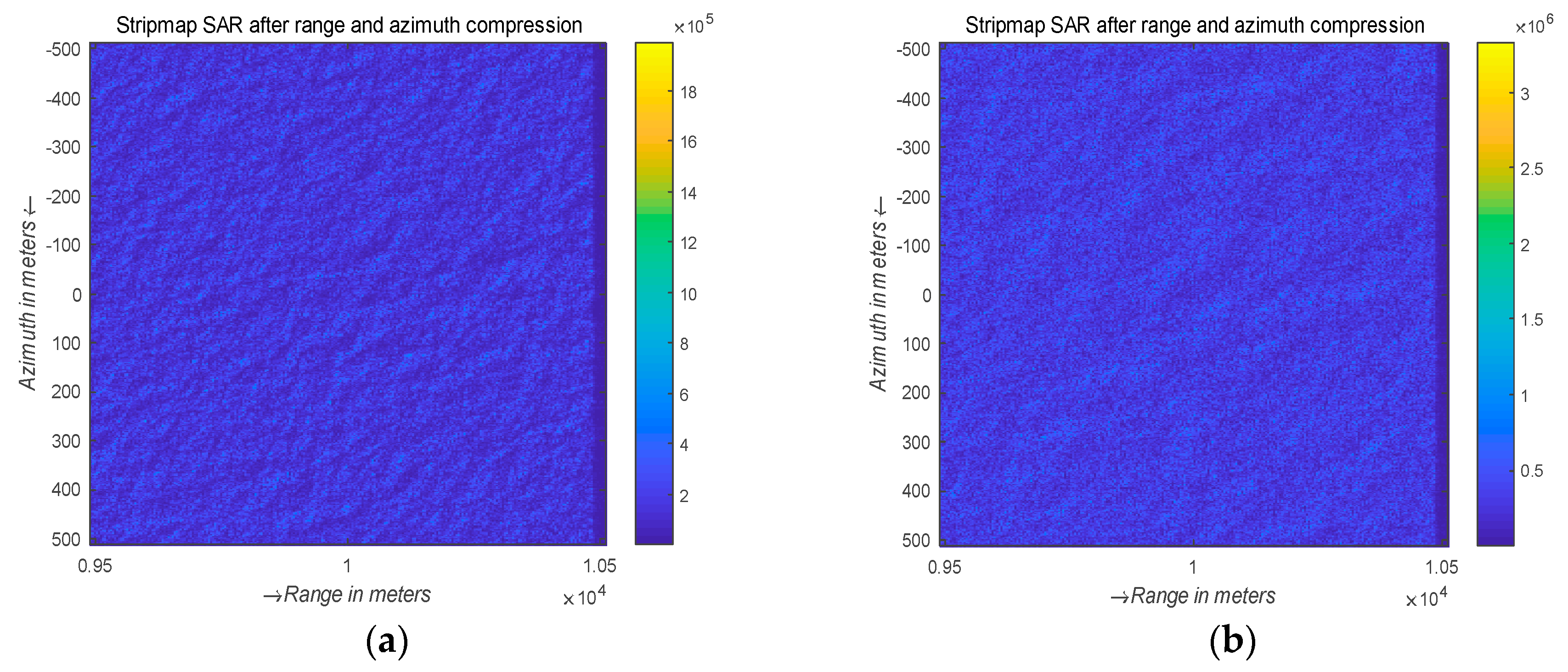
2.4. SAR Imaging of the Ocean Surface

In this paper, ocean surface echo signals were processed by the Range–Doppler (RD) imaging algorithm to obtain ocean SAR images. The RD algorithm consists of three key steps, namely, range compression, range migration correction, and azimuth compression, and the RD algorithm obtains high resolutions in the range and azimuth by pulse compression [31,32].

3. Results and Analysis

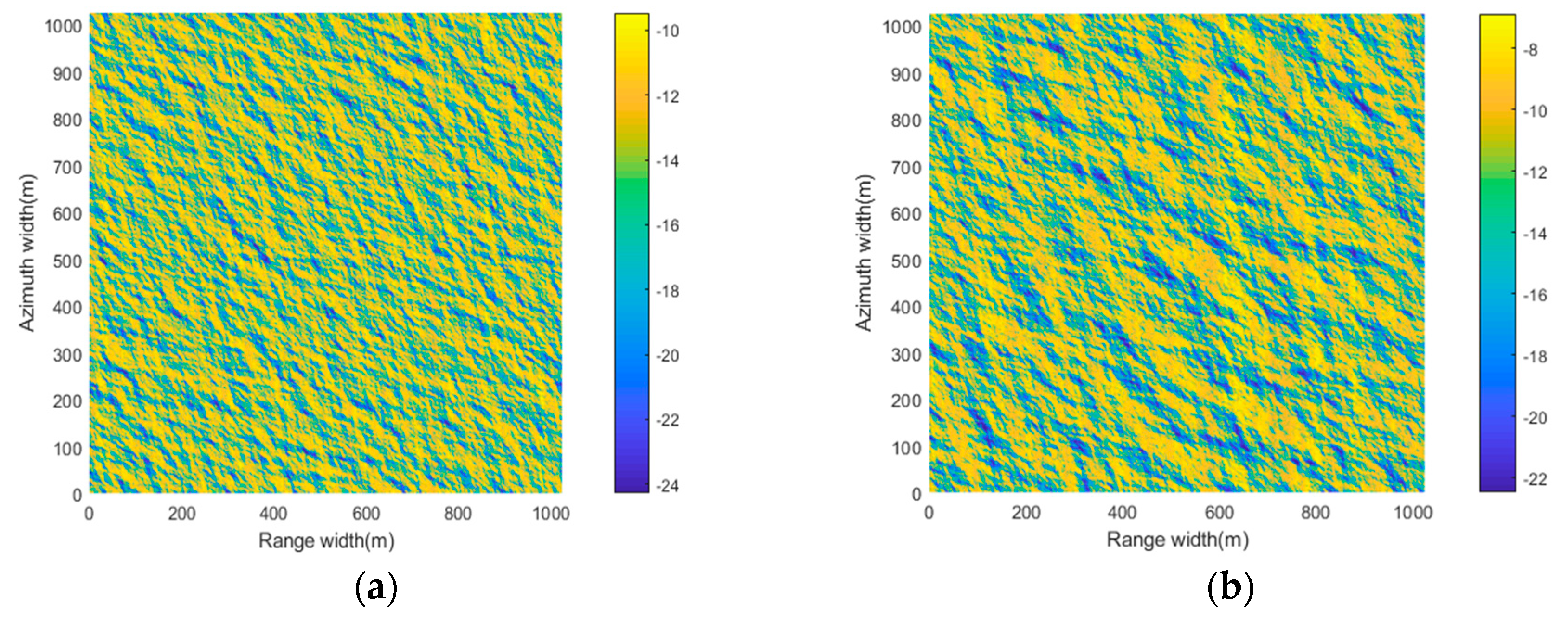
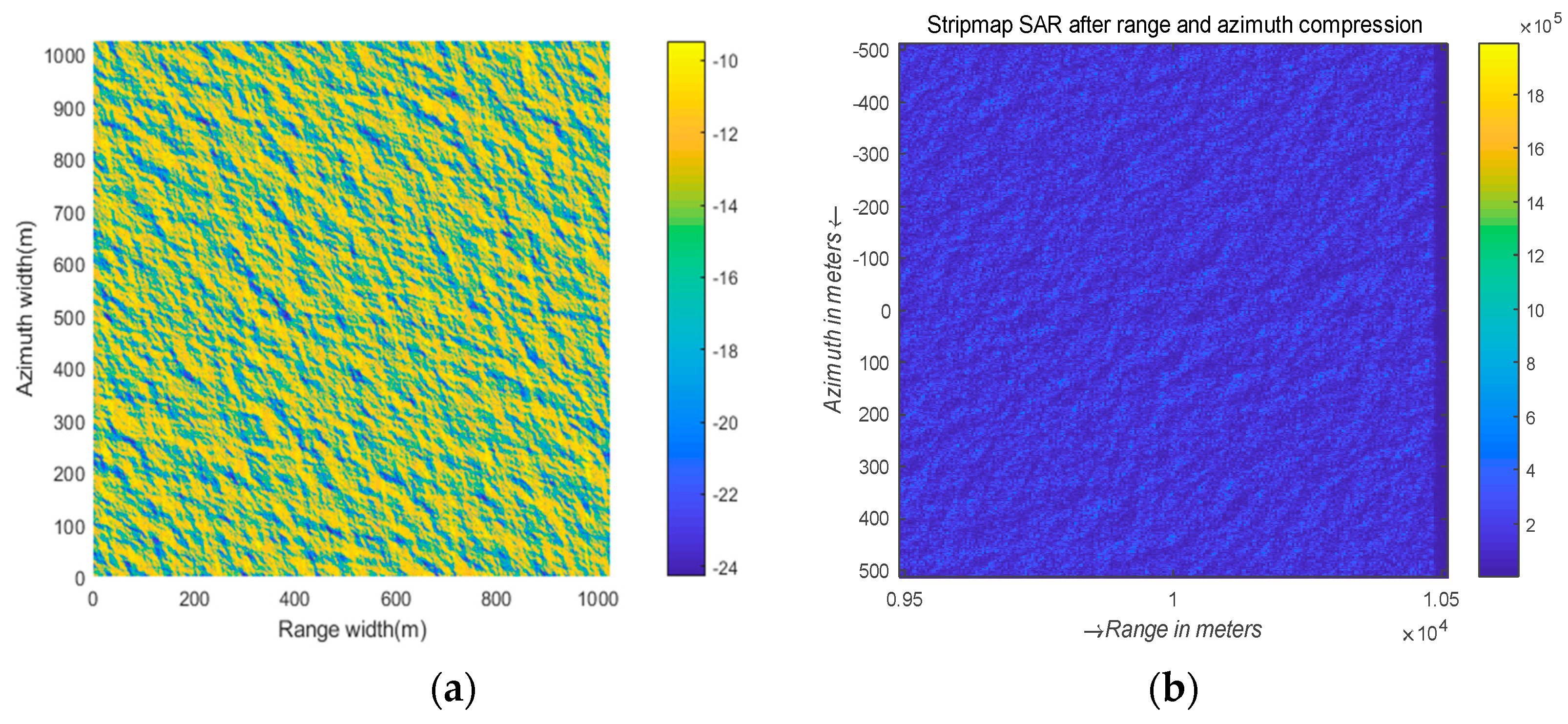
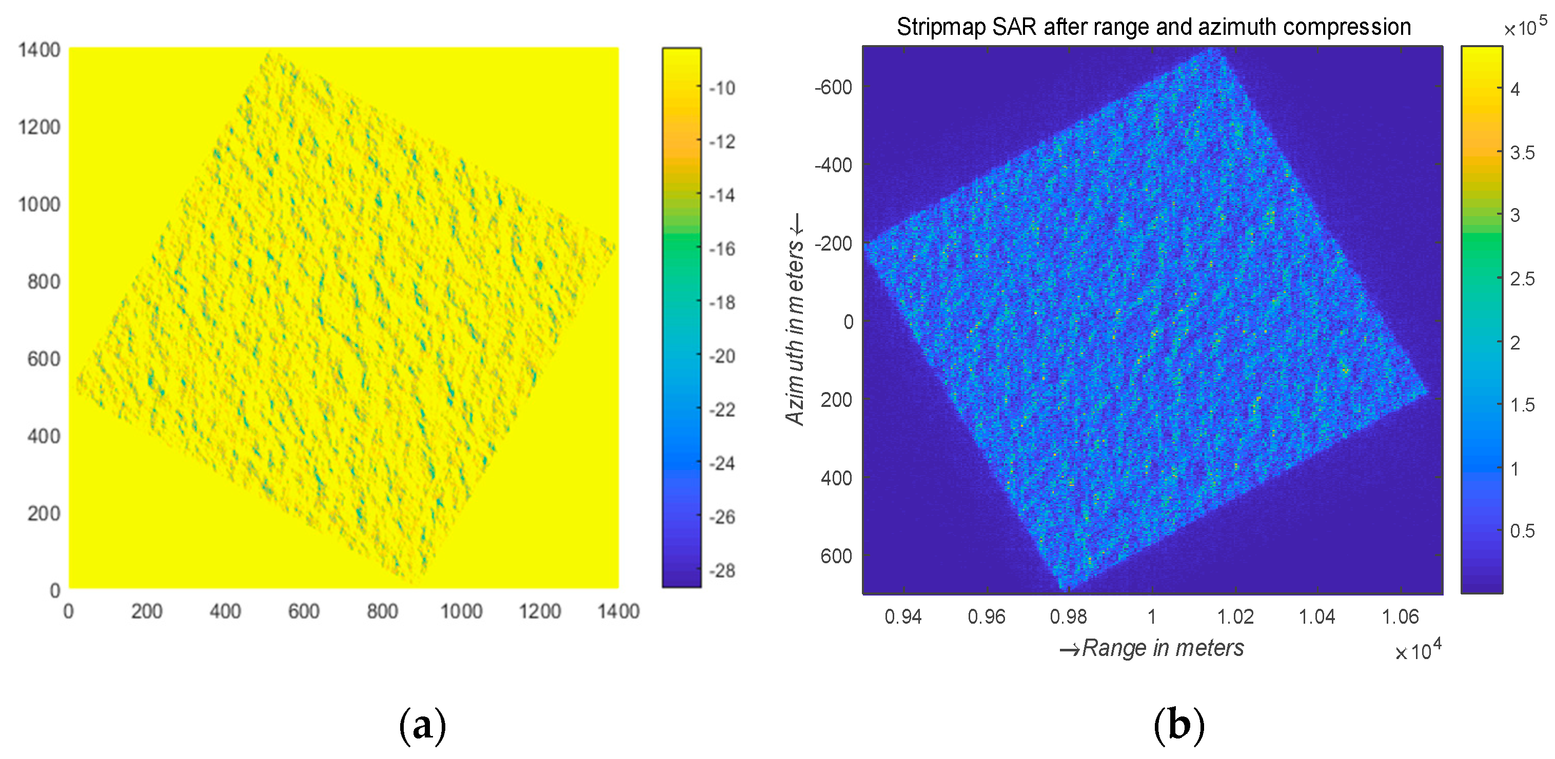
3.1. Analysis of the Single-SAR Imaging Simulation Results

Wind speeds of 10 m/s, 13 m/s, and 15 m/s were assigned Equation (1), and the 1D PM spectrum was simulated, as shown in Figure 1. It can be seen from the figure that although the spectrum in theory includes the constituent waves with frequencies from zero to infinity, a significant portion of the spectrum is concentrated in only a narrow frequency range. The wave height and the period range increase as the wind speed increases, and the position of the peak shifts in the direction of low frequency [33].

A wind direction angle of 45° and wind speeds of 10 m/s and 15 m/s at a height of 10 m were assigned to Equation (4), and the 2D PM wave spectra were simulated. The spectra are shown in the figures below. Wind direction angle is regarded as the direction of wave propagation, defined as the angle to the range direction. The range of the wavenumbers in the azimuth and range directions is determined by the size of the ocean surface and the sampling interval. The color bars on the right side of the figures represent the magnitude of the wavenumber spectrum and represent the energy of the wavenumber spectrum. It can be seen from Figure 2a,b that when the sampling pitch is constant, the wind speed is higher, and the energy of the wave spectrum is stronger and more concentrated. Figure 2a,c show that when the wind speed is constant, the sampling interval is larger and the wavenumber range is smaller. The sampling pitch is inversely proportional to the wavenumber range. According to Figure 1 and the gravity dispersion relation ${\omega }^2=kg$, it can be concluded that the higher the wind speed is, the smaller the wavenumber range corresponding to the PM spectrum.

The 2D ocean surface was simulated by using the 2D PM wave spectrum as the spectral model, as shown in Figure 3a,b. These results are based on Equations (5) and (6). The ocean surface area size is 1024 m × 1024 m, which can be adjusted according to the actual needs, but it is recommended to set the area size to the power of two to facilitate the subsequent FFT. Since the wave propagation direction is perpendicular to the wave stripe, the wave propagation direction in the figure is 45°, which is in accordance with the initial input conditions of the simulation. Moreover, the height fluctuation of the sea surface increases with increasing wind speed, which is consistent with the variation characteristics of the real ocean surface. This result confirms the effectiveness of the Monte Carlo method.

The ocean surface backscattering coefficient of wind speeds of 10 m/s and 15 m/s could be obtained by Equations (7)–(9), as shown in Figure 4. The stripe trend of the backscattering coefficient is basically consistent with the streak trend of the corresponding ocean surface. The trend can show the variation in ocean surface fluctuation by the brightness levels of the trough and the peak, which proves that it is feasible to calculate the ocean surface backscatter coefficient by the two-scale model.

After calculating the backscattering coefficient, the ocean surface echo signals were calculated based on Equations (10) and (11), as shown in Figure 5. The figure does not show any information about the ocean surface. This condition exists because the original echo signals are obscure and must be processed by the imaging algorithm to obtain feature information of the imaging target from the SAR images.

When a SAR images the ocean surface, the scanning band generated by the electromagnetic wave needs to sweep across the ocean surface; that is, the ocean surface needs to be located in the SAR imaging coordinate system. Since the simulated ocean area was approximately 1 km × 1 km, for the SAR, the width was small enough to cause ground bending. Therefore, without considering factors such as the rotation of the Earth and curvature of the ground and taking the subsatellite point as the origin, the projections of the SAR azimuth and range were the x and y axes, and the SAR imaging coordinate system was established. The reason for establishing the coordinate system in this way is that the azimuth and range are perpendicular to each other. Other parameters of the SAR system are the same as those in

Table 1. System parameters.

Parameters	Numerical Value
Platform height	10 km
Speed	200 m/s
Observation angle of incidence	30°
Carrier frequency	3 GHz
Pulse duration	5 μs
Chirp frequency modulation bandwidth	18.75 MHz

.

The ocean surface SAR images obtained by the RD algorithm are shown in Figure 6. The direction of the wave stripe in the figure represents the direction of wave travel, and this direction is the same as those of the initial input parameters of the simulation.

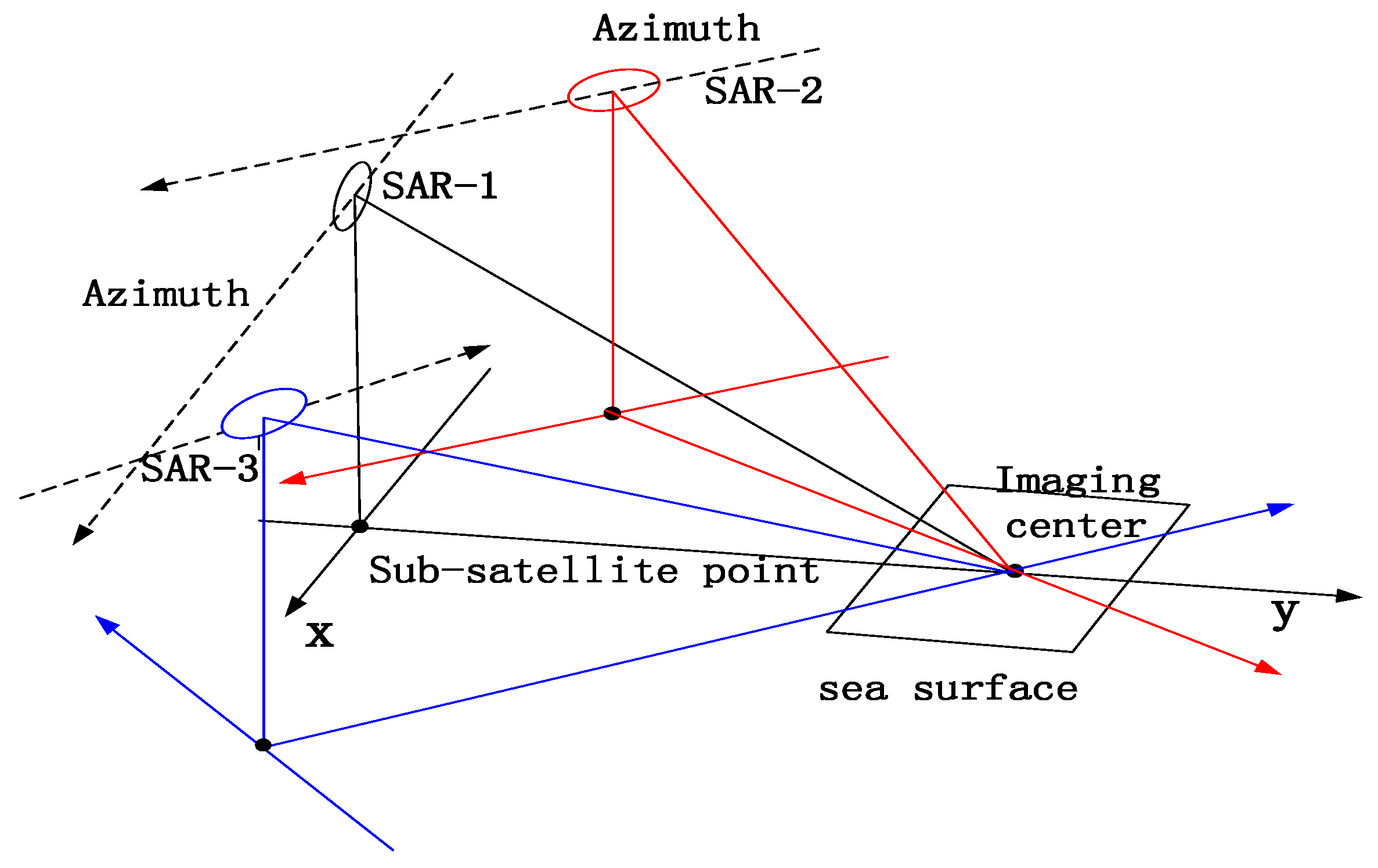
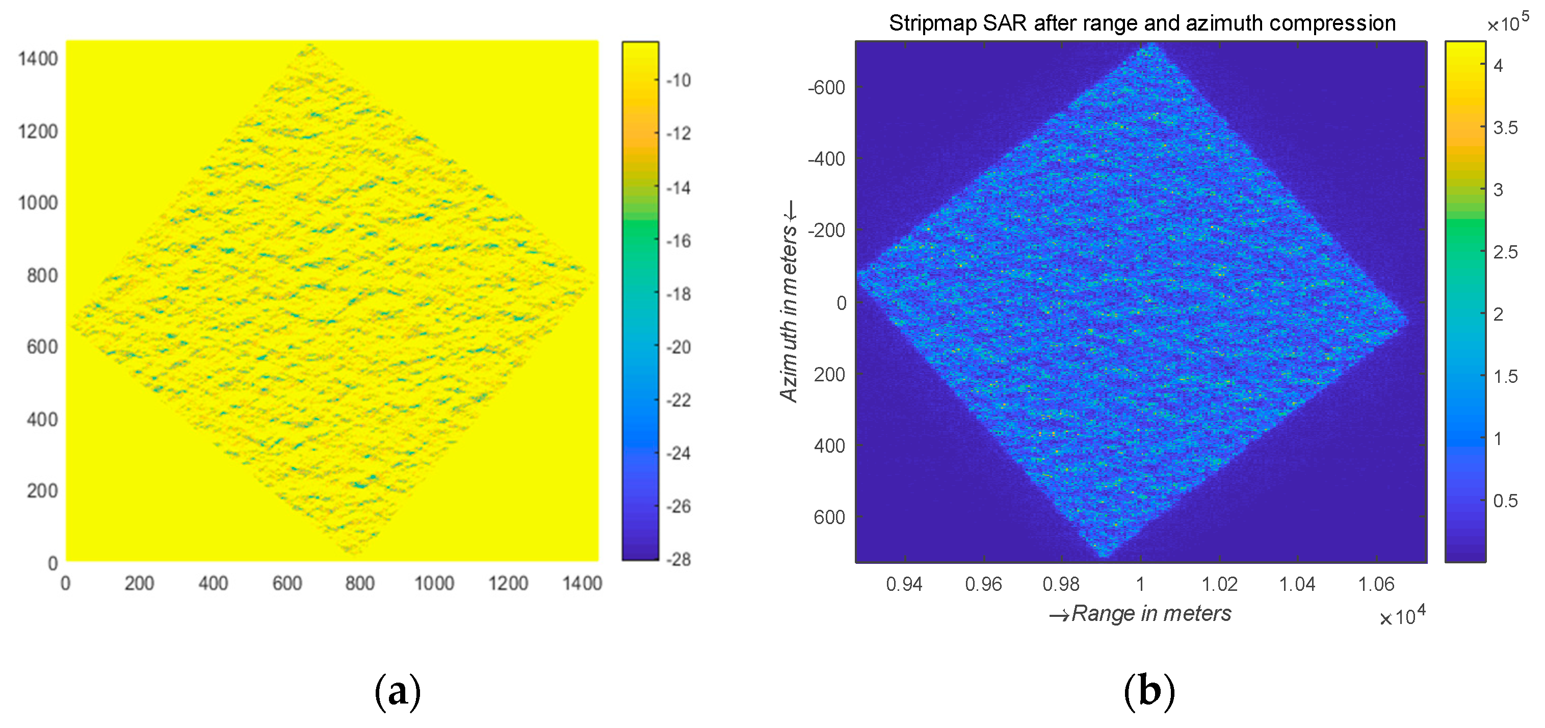
3.2. Simulation of Networked SAR Satellites and Multiview Ocean Wave SAR Synchronization Data

In this paper, a virtual network of satellites consisting of three SARs was simulated, and the SAR synchronized observation data of different orbit directions were simulated by the networked satellite cooperative observation. The SAR that implemented the imaging simulation in the previous section is called SAR-1. Based on the parameters and working principle of SAR-1, the other two SARs with angles of 30° and −50° from the flight direction of SAR-1 were simulated. The angle was positive in the same direction as SAR-1 and negative in the reverse flight. The satellites were named SAR-2 and SAR-3. The SAR-2 and SAR-3 working modes were also side-looking. Based on SAR-1, the position coordinates of the subsatellite point were changed, and the angle of orbit was adjusted according to the relative position between the subsatellite points while ignoring the Earth’s rotation and ground bending. A schematic diagram of the three SAR observations in the same sea area is shown in Figure 7.

The backscattering coefficient images obtained by the networked SAR satellite observations of the ocean surface and the corresponding ocean SAR images are shown in the following figures.

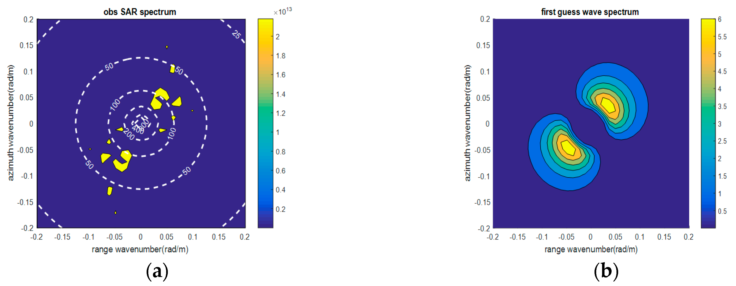
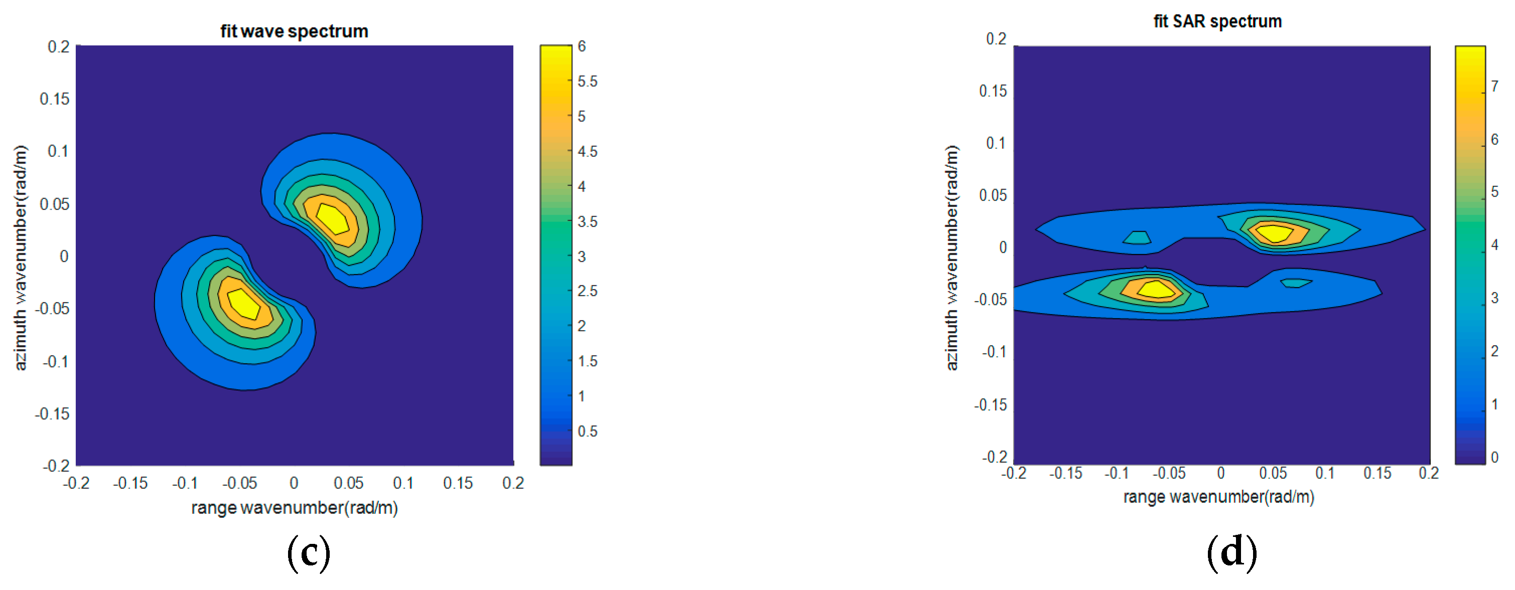
3.3. Accuracy Assessment of the Multiview Ocean Wave SAR Synchronization Data

In Section 3.1 and Section 3.2, we showed the results of the networked SAR imaging simulation, but the feasibility of the data is not clear. In this section, we would evaluate the accuracy of the data to show that the data are usable. For simulated SAR imaging data, the backscatter coefficients are equivalent to the input parameters, and the echo signals are generated in the middle of the simulation process. With this in mind, we only evaluate the accuracy of the backscatter coefficients and the ocean surface SAR images.

The value of the backscatter coefficients is related to the roughness of the ocean surface, while the surface roughness is determined by the wind speed. Therefore, wind speed is the key factor affecting the backscatter coefficients of the ocean surface. When the incident angle of the SAR beam is fixed with the angle of wind direction, the backscatter coefficient increases with the increase of wind speed, however, the growth rate of backscatter coefficient decreases [34]. As can be seen from Figure 4, when the wind speed increases, the backscatter coefficients increase indeed. The simulated results are in agreement with the theory, indicating that the accuracy of the simulated backscattering coefficients is relatively high. As initial input parameters, the accuracy of backscatter coefficients can also be verified by the simulated ocean wave data.

In order to analyze the accuracy of the simulated ocean wave data, we used the Max Plank Institute (MPI) algorithm [35] to invert the wave spectrum of ocean wave data. The MPI algorithm is derived describing the mapping of a 2D ocean wave spectrum into a SAR image spectrum. The inversion results of the ocean wave data observed by SAR-1 are shown in the figures below.

As can be seen from the figures, the direction of wave propagation is consistent with the initial input angle. The first guess wave spectrum is in line with the magnitude and shape of the fit wave spectrum. The fit SAR spectrum is also consistent with the magnitude of the fit wave spectrum. The above phenomenon shows that the wave spectrum inverted from the ocean wave data is ideal.

For SAR-2, the wave propagation direction is the same as the SAR-1, which is also 45°. The orbital angle of SAR-2 and SAR-1 is 30°, and it can be calculated that the angle between the wave propagation direction and the range direction of SAR-2 is 75°. The inversion results of ocean wave data observed by SAR-2 are shown in the figures below.

For SAR-3, the wave propagation direction is also 45°. The orbital angle of SAR-3 and SAR-1 is −50°, and it can be calculated that the angle between the wave propagation direction and the range direction of SAR-3 is 5°. The inversion results of ocean wave data observed by SAR-3 are shown in the figures below.

As can be seen from Figures 11–13, the SAR wave synchronization data obtained by networked SAR satellites can invert the fit wave spectrum and the fit SAR spectrum, ideally. In this way, it can be proved that the accuracy of the SAR imaging simulation data is relatively high.

4. Discussion

In Section 3.1, we analyzed the results of each step of the imaging simulation in detail. The results showed that the ocean surface undulations at different wind speeds are different, reflecting the influence of the wind speed on the ocean surface undulations and conforming to real ocean characteristics, which also proves the effectiveness of the imaging simulation results. The calculation of the echo signals is a difficult problem in the whole SAR imaging simulation process. At present, the echo simulation of point targets is mostly realized in the research work, while the echo simulation of area targets such as the ocean surface is seldom realized. The ocean surface SAR echo simulation in this paper can provide a reference for research work in related fields.

During simulation, discretization of the constructed ocean surface was considered to be a combination of a series of discrete points. Using the discrete ocean surface as the background field, the slope at each point of the ocean surface was calculated. The backscattering coefficients of all points on the ocean surface were calculated according to the slope, and the calculation method had a high precision. Range migration bending is clearly related to the range and azimuth sampling points. The larger the slant distance or the wider the scanning beam is, the wider the range of the sampling points. The longer the synthetic aperture time or the higher the pulse repetition frequency is, the more azimuth sampling points there are. The larger the number of sampling points is, the more notable the range migration is, and the greater the calculation amount is. In the case that the accuracy of the data is not high, range migration correction can be omitted to reduce the amount of calculation.

In Section 3.2, we analyzed the simulation of networked satellites and multiview ocean wave SAR synchronization data in detail. The results showed that the difficulty of simulating was to ensure that the orbits of the three SARs were at an angle based on the orbital parameters of the SARs. After the simulation of the networked satellites, the most important and innovative part of this paper is the generation of the multiview SAR wave synchronization data. The key to this process is that the three SARs can simultaneously observe the same sea area. The working mode of the SAR can be regarded as the stop-go-stop model; therefore, we can make the electromagnetic pulse emission times of the three SARs the same to ensure simultaneous observations. According to Section 2.2, we can summarize the specific steps of the Monte Carlo method. First, the 2D Gaussian white noise is simulated, and then the noise is linearly filtered by the 2D wave spectrum to obtain the FFT of the ocean surface height fluctuation function, and the ocean surface height fluctuation function can be obtained by IFFT. No time factor was added during the ocean simulation, so the Monte Carlo method is used to simulate the freezing ocean surface. Networked SAR satellites can acquire synchronized observation data at the same time and the same place during imaging simulation.

Figure 8, Figure 9 and Figure 10 demonstrate that the ocean surface SAR images and the backscatter coefficient images are horizontally symmetric. This result is because the RD algorithm performs FFTs and IFFTs on the azimuths and ranges of the echo signals, respectively. That’s why the observed SAR spectrum is flipped horizontally. When the SAR images are horizontally flipped, the wave stripe trends of the SAR images are basically the same as the stripe trends of the backscattering coefficient figures, but the degrees of blur are different. This situation is consistent with real ocean physical characteristics.

It can also be seen that for the same sea area, the results observed by the SAR for different flight directions are different, and the clarity of the wave stripes is related to the flight direction of the SAR. Velocity bunching modulation and ocean scene coherence time are the essential causes of the azimuth cutoff. The angle between the direction of wave propagation and the direction of SAR flight is a key factor affecting the azimuth cutoff. When the direction of wave propagation is fixed, the different SAR flight directions have different effects on the azimuth cutoff wavelength. The manifestation in the SAR images is that the images become blurred, and the wave information whose wavelength is smaller than the azimuth cutoff wavelength is lost. However, the degree of azimuth cutoff cannot be intuitively judged from the SAR images. Currently, there is no clear equation for calculating the azimuth cutoff wavelength, which can only be estimated by parameters such as the SWH, wind speed and range-to-velocity ratio (R/V). In future research, wave spectrum inversion can be realized based on simulated SAR data and compared with the buoy omnidirectional spectrum or wave spectrum data provided by the European Centre for Medium-Range Weather Forecasts (ECMWF) to study the energy loss under different degrees of azimuth cutoff. The compensation of the azimuth cutoff wavelength can be realized based on multiview SAR wave synchronization data.

In Section 3.3, we analyzed the accuracy of the SAR wave synchronization data obtained by networked SAR satellites. The results showed that the variation of the backscattering coefficients with wind speed is consistent with the theory. In addition, the results reflected in Figure 11, Figure 12 and Figure 13 verify the accuracy of the simulated SAR ocean wave data. In particular, the shape of the fit SAR spectrum is compressed upward in the azimuth direction. Waves with wavelengths less than a certain value cannot be imaged, which also reflects the effect of azimuth cutoff on SAR imaging. There is another thing that needs to be noted. The results of observed SAR spectrum were obtained through flip horizontal. The reason is derived from the analysis of Figure 8, Figure 9 and Figure 10.

5. Conclusions

In this paper, we simulated ocean surface images from a single SAR satellite at different wind speeds and analyzed the effects of the different wind speeds on the images. The main methods used in this paper were the rough sea model, electromagnetic scattering model, time-domain echo algorithm and imaging algorithm. Aimed at the problem of the azimuth cutoff of ocean waves observed by SARs, networked SAR satellites with three SARs were simulated, and multiview SAR wave synchronization data were obtained, which is the innovation and difficulty of this paper. MPI algorithm was used to verify the accuracy of the SAR multiview wave synchronization data. Although the calculations of complex original echo signals are not avoided, the accuracy of the obtained sea surface SAR images is high. The conclusions that we have reached are as follows:

Firstly, wind speed is the key factor affecting ocean surface fluctuation and backscatter coefficients, and the change trend of stripe can be seen from SAR images.

Secondly, ocean surface SAR images and the backscatter coefficient images are horizontally symmetric. This situation causes the observed SAR spectrum to be horizontally flipped.

Thirdly, azimuth cutoff has a non-linear effect on SAR images, and this effect is irreversible. From the fit SAR spectrum obtained from the MPI algorithm inversion, the influence of the azimuth cutoff can be seen. SAR can only image the ocean waves within a certain wavenumber range, and waves with wavelengths less than the azimuth cutoff wavelength cannot be imaged.

To sum up, the simulation of the multiview SAR ocean wave synchronization data in this paper has important significance in the imaging algorithm research and SAR system scheme design, and we believe that the results in this paper can provide some reference for marine remote sensing. The acquired data can also be used as the basic data source for related research, such as the azimuth cutoff wavelength compensation.

References

1. Li, X.M.; Lehner, S.; Bruns, T. Ocean Wave Integral Parameter Measurements Using Envisat ASAR Wave Mode Data. IEEE Trans. Geosci. Remote Sens. 2010, 49, 155–174. [Google Scholar] [CrossRef] [Green Version]
2. Rani, S.I.; Das Gupta, M.; Sharma, P.; Prasad, V.S. Intercomparison of Oceansat-2 and ASCAT Winds with In Situ Buoy Observations and Short-Term Numerical Forecasts. Atmos. Ocean 2014, 52, 92–102. [Google Scholar] [CrossRef] [Green Version]
3. Tang, W.; Yueh, S.H.; Fore, A.G.; Hayashi, A. Validation of Aquarius sea surface salinity with in situ measurements from Argo floats and moored buoys. J. Geophys. Res. Oceans 2014, 119, 6171–6189. [Google Scholar] [CrossRef]
4. Han, W.X.; Yang, J.G.; Wang, J.Z. Calibration and evaluation of satellite radar altimeter wave heights with in situ buoy data. Acta Oceanol. Sin. 2016, 38, 73–89. [Google Scholar]
5. Shaeb, K.H.B.; Anand, A.; Joshi, A.K.; Bhandari, S.M. Comparison of Near Coastal Significant Wave Height Measurements from SARAL/AltiKa with Wave Rider Buoys in the Indian Region. Mar. Geod. 2015, 38, 422–436. [Google Scholar] [CrossRef]
6. Woo, H.J.; Park, K.A. Long-term trend of satellite-observed significant wave height and impact on ecosystem in the East/Japan Sea. Deep Sea Res. Part II Top. Stud. Oceanogr. 2016, 143, 1–14. [Google Scholar] [CrossRef]
7. Mathew, T.; Chakraborty, A.; Sarkar, A.; Kumar, R. Comparison of oceanic winds measured by space-borne scatterometers and altimeters. Remote Sens. Lett. 2012, 3, 6. [Google Scholar] [CrossRef]
8. Kim, D.J.; Moon, W.M.; Moller, D.; Imel, D.A. Measurements of ocean surface waves and currents using L- and C-band along-track interferometric SAR. IEEE Trans. Geosci. Remote Sens. 2003, 41, 2821–2832. [Google Scholar]
9. Zhang, B.; Perrie, W.; He, Y.J. Validation of RADARSAT-2 fully polarimetric SAR measurements of ocean surface waves. J. Geophys. Res. Oceans 2010, 115. [Google Scholar] [CrossRef]
10. Lehner, S.; Pleskachevsky, A.; Gebhardt, C.; Rosenthal, W.; Bruns, T.; Hoffmann, P.; Kieser, J. High resolution wind and wave measurements from TerraSAR-X and Tandem-X satellites in comparison to marine forecast. In Proceedings of the 2015 IEEE International Geoscience and Remote Sensing Symposium (IGARSS), Milan, Italy, 26–31 July 2015; pp. 2519–2522. [Google Scholar]
11. Yoshida, T.; Rheem, C.K. SAR Image Simulation in the Time Domain for Moving Ocean Surfaces. Sensors 2013, 13, 4450–4467. [Google Scholar] [CrossRef] [Green Version]
12. Lin, B.; Shao, W.; Li, X.; Li, H.; Du, X.; Ji, Q.; Cai, L. Development and validation of an ocean wave retrieval algorithm for VV-polarization Sentinel-1 SAR data. Acta Oceanol. Sin. 2017, 36, 95–101. [Google Scholar] [CrossRef]
13. Grieco, G.; Lin, W.; Migliaccio, M.; Nirchio, F.; Portabella, M. Dependency of the Sentinel-1 azimuth wavelength cut-off on significant wave height and wind speed. Int. J. Remote Sens. 2016, 37, 5086–5104. [Google Scholar] [CrossRef]
14. Dowd, M.; Vachon, P.W.; Dobson, F.W.; Olsen, R.B. Ocean wave extraction from RADARSAT synthetic aperture radar inter-look image cross-spectra. IEEE Trans. Geosci. Remote Sens. 2002, 39, 21–37. [Google Scholar] [CrossRef]
15. Kerbaol, V.; Chapron, B.; El Fouhaily, T.; Garello, R. Fetch and wind dependence of SAR azimuth cutoff and higher order statistics in a mistral wind case. In Proceedings of the 1996 International Geoscience and Remote Sensing Symposium (IGARSS’96), Lincoln, NE, USA, 31 May 1996. [Google Scholar]
16. Ren, L.; Yang, J.S.; Zheng, G.; Wang, J. Significant wave height estimation using azimuth cutoff of C-band RADARSAT-2 single-polarization SAR images. Acta Oceanol. Sin. 2015, 34, 93–101. [Google Scholar] [CrossRef]
17. Stopa, J.E.; Ardhuin, F.; Chapron, B.; Collard, F. Estimating wave orbital velocity through the azimuth cutoff from space-borne satellites. J. Geophys. Res. Oceans 2015, 120, 7616–7634. [Google Scholar] [CrossRef]
18. Liu, B.C.; He, Y.J. SAR Raw Data Simulation for Ocean Scenes Using Inverse Omega-K Algorithm. IEEE Trans. Geosci. Remote Sens. 2016, 54, 6151–6169. [Google Scholar] [CrossRef]
19. Zhao, Z.Q.; Luo, X.Y.; Nie, Z.P. Simulation of polarization SAR imaging of sea wave using two-Scale model. J. Univ. Electron. Sci. Technol. China 2009, 38, 651–655. [Google Scholar]
20. Guo, D.; YU, T.; Fernado, N. Simulation of polarization SAR imaging of ocean surface based on the two-scale model. J. Electron. Meas. Instrum. 2011, 25, 81–88. [Google Scholar] [CrossRef]
21. Franceschetti, G.; Migliaccio, M.; Riccio, D. On ocean SAR raw signal simulation. IEEE Trans. Geosci. Remote Sens. 1998, 36, 84–100. [Google Scholar] [CrossRef]
22. Zhu, M.B.; Zou, J.W.; Dong, W. Imaging simulation of dynamic sea surface with missile-borne SAR. Chin. J. Radio Sci. 2012, 3, 592–597. [Google Scholar]
23. Fan, W.N.; Zhang, M.; Li, J.X. Highly squinted SAR imaging simulation of ship-ocean scene based on EM scattering mechanism. IET Microw. Antennas Propag. 2018, 12, 1160–1165. [Google Scholar] [CrossRef]
24. Xu, X.J.; Li, X.F. Radar Phenomenological Models for Ships on Time-Evolving Sea Surface; National Defense Industry Press: Beijing, China, 2013; pp. 5–6. [Google Scholar]
25. Mao, C.; Qiu, Z.M.; Liu, Z.; Lu, F.X. Monte Carlo simulation of three-dimensional random rough sea surface. Ship Sci. Technol. 2013, 35, 25–28. [Google Scholar]
26. He, Z.H. Study on Ocean Modeling, Imaging and Along-Track InSAR. Master’s Thesis, National University of Defense Technology, Hunan, China, 2007. [Google Scholar]
27. Huang, Y.K. Modeling Simulation and System Design of Synthetic Aperture Radar Echo Simulator. Master’s Thesis, University of Electronic Science and Technology of China, Sichuan, China, 2008. [Google Scholar]
28. Klein, L.; Swift, C.T. An improved model for the dielectric constant of sea water at microwave frequencies. IEEE Trans. Antennas Propag. 2003, 25, 104–111. [Google Scholar] [CrossRef]
29. Zhang, Y.D. Study on Electromagnetic and Light Scattering Characteristics of Sea Surface. Ph.D. Thesis, Xidian University, Shanxi, China, 2004. [Google Scholar]
30. Guo, D. SAR Imaging Simulations Based on the Ocean Scenes and The Electromagnetic Scattering Study. Ph.D. Thesis, University of Electronic Science and Technology of China, Sichuan, China, 2011. [Google Scholar]
31. Pi, Y.M.; Yang, J.Y.; Fu, Y.S.; Yang, X.B. Synthetic Aperture Radar Imaging Principle; University of Electronic Science and Technology of China Press: Sichuan, China, 2007; pp. 78–82. [Google Scholar]
32. Cumming, I.G.; Wong, F.H. Digital Processing of Synthetic Aperture Radar Data: Algorithhms and Implementation; Publishing house of electronics industry: Beijng, China, 2012; pp. 154–166. [Google Scholar]
33. Wen, S.C.; Yu, Z.W. Wave Theory and Calculation Principle; Science Press: Beijing, China, 1984; pp. 142–149. [Google Scholar]
34. Hersbach, H.; Stoffelen, A.; Haan, S.D. An improved C-band scatterometer ocean geophysical model function: CMOD5. J. Geophys. Res. Oceans 2007, 112. [Google Scholar] [CrossRef]
35. Hasselmann, K.; Hasselmann, S. On the nonlinear mapping of an ocean wave spectrum into a synthetic aperture radar image spectrum and its inversion. J. Geophys. Res. 1991, 96, 10713. [Google Scholar] [CrossRef]
Figure 1. The one-dimensional (1D) Pierson Moskowitz (PM) spectra at different wind speeds.
Jmse 07 00180 g001
Figure 2. Two-dimensional (2D) PM wavenumber spectrum as follows: (a) 2D PM wavenumber spectrum at a wind speed of 10 m/s and a sampling pitch of 8 m, (b) 2D PM wavenumber spectrum at a wind speed of 15 m/s and a sampling pitch of 8 m, and (c) 2D PM wavenumber spectrum at a wind speed of 10 m/s and a sampling distance of 16 m.
Jmse 07 00180 g002
Figure 3. 2D ocean surface diagram as follows: (a) 2D sea surface at a wind speed of 10 m/s, (b) top view of (a), (c) 2D sea surface at a wind speed of 15 m/s, and (d) top view of (c). The color bars on the right side of the figure represent the height fluctuations of the ocean surface.
Jmse 07 00180 g003
Figure 4. Ocean surface backscatter coefficient as follows: (a) wind speed of 10 m/s and (b) wind speed of 15 m/s.
Jmse 07 00180 g004
Figure 5. Ocean surface echo signals as follows: (a) wind speed of 10 m/s and (b) wind speed of 15 m/s.
Jmse 07 00180 g005
Figure 6. Ocean surface synthetic aperture radar (SAR) images as follows: (a) wind speed of 10 m/s and (b) wind speed of 15 m/s.
Jmse 07 00180 g006
Figure 7. Networked SAR satellite observations of the same sea area.
Jmse 07 00180 g007
Figure 8. Data observed by SAR-1 as follows: (a) ocean surface backscattering coefficient and (b) ocean SAR image.
Jmse 07 00180 g008
Figure 9. Data observed by SAR-2 as follows: (a) ocean surface backscattering coefficient and (b) ocean SAR image.
Jmse 07 00180 g009
Figure 10. Data observed by SAR-3 as follows: (a) ocean surface backscattering coefficient and (b) ocean SAR image.
Jmse 07 00180 g010
Figure 11. SAR-1: Max Plank Institute (MPI) algorithm inversion results as follows: (a) Observed SAR spectrum (after horizontal flip), (b) first guess PM wave spectrum, (c) fit PM wave spectrum, and (d) fit SAR spectrum.
Jmse 07 00180 g011aJmse 07 00180 g011b
Figure 12. SAR-2: MPI algorithm inversion results as follows: (a) Observed SAR spectrum (after horizontal flip), (b) first guess PM wave spectrum, (c) fit PM wave spectrum, and (d) fit SAR spectrum.
Jmse 07 00180 g012
Figure 13. SAR-3: MPI algorithm inversion results as follows: (a) Observed SAR spectrum (after horizontal flip), (b) first guess PM wave spectrum, (c) fit PM wave spectrum, and (d) fit SAR spectrum.
Jmse 07 00180 g013