Efficient Image Registration for Underwater Optical Mapping Using Geometric Invariants


Abstract
1. Introduction
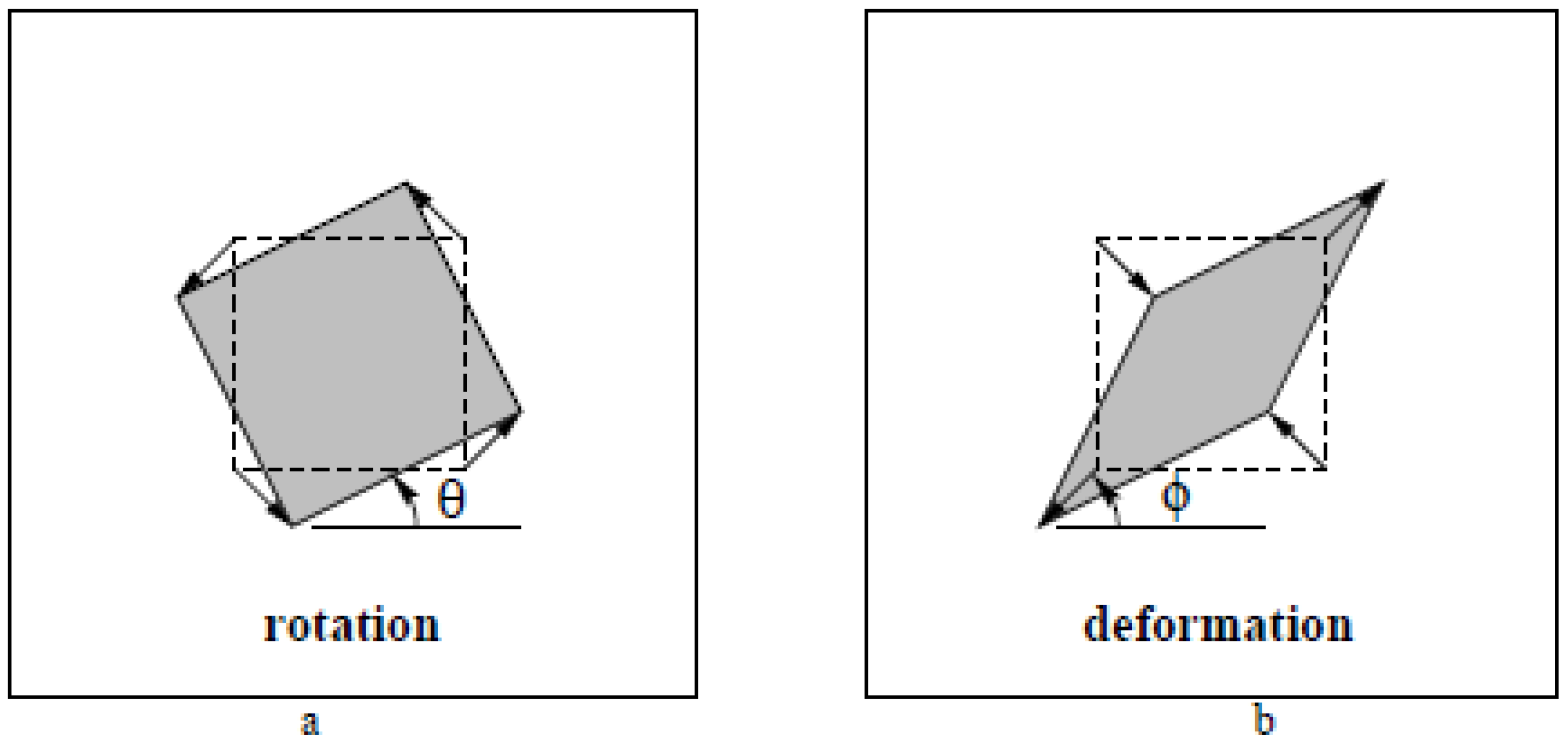
2. Overview of Used Planar Transformations
- Similarity Transformations
- A Similarity transformation is a scale included version of Euclidean transformation. The rotation is around an optical axis and scale in our context refers to the altitude changes of an underwater robot. A similarity transformation can be decomposed as follows [3]:where is for rotation, s is uniform scaling on both the x- and y-axes while is a translation vector making four DOFs in total.
- Affine Transformations
- An affine transformation has six DOFs and it can be decomposed as follows [3]:where is the rotations and non-isotropic scalings while is the translation on the x- and y-axes. Further decomposition of can be done as follows:
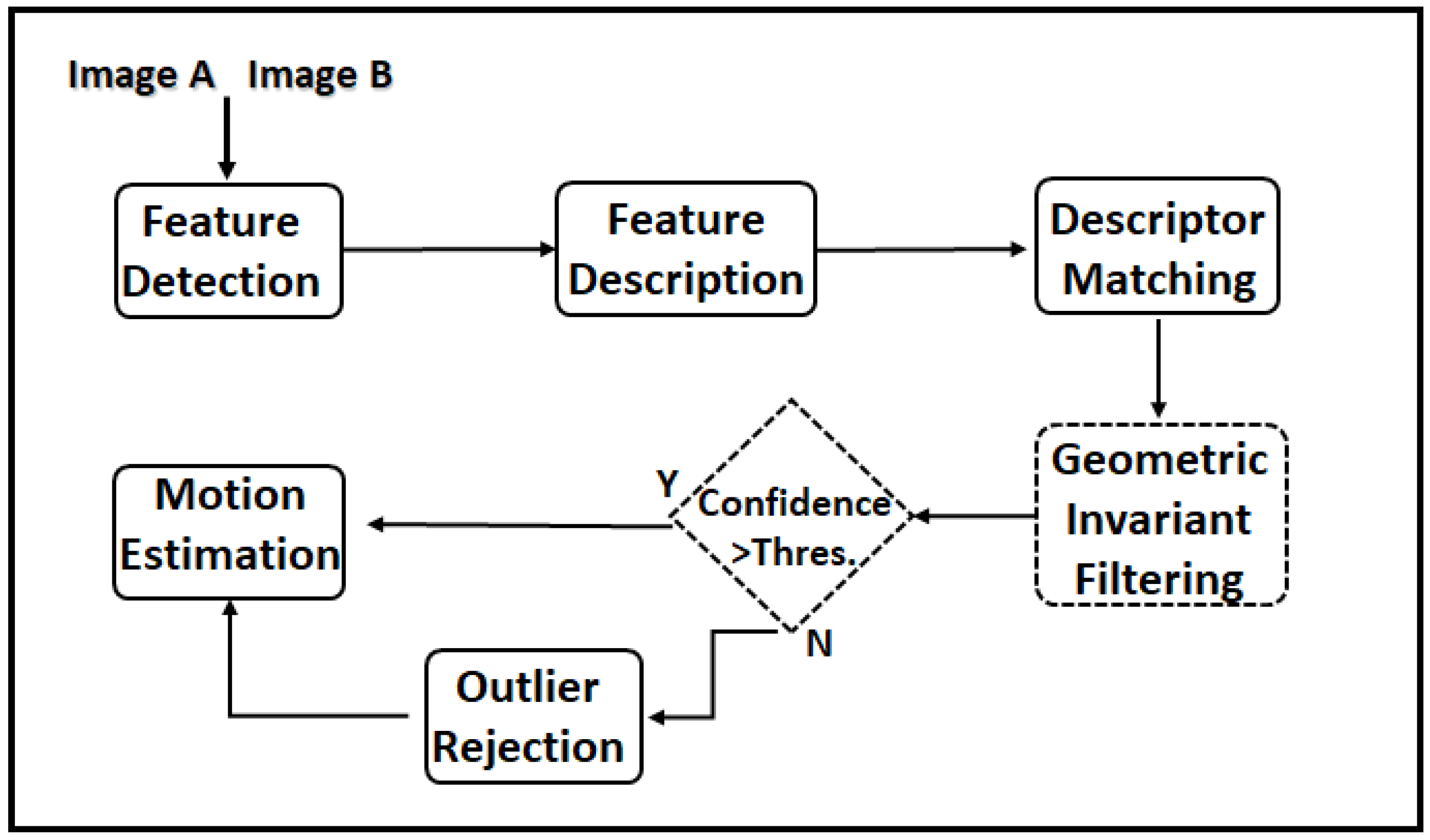
3. Geometrical Invariant Extraction from Overlapping Images
- Ratio of Lengths
- We compute the distance between all matched points in the same image:where and . Since we are interested in the ratio of lengths, we compute . If the feature matching was free of outliers, the computed r values would be the same and/or very close to each other. Some extreme values are filtered out (e.g., ) assuming that the ratio does not have such extreme values. In order to find a ratio of lengths, we compute the median of r values. As r values may suffer truncation and/or rounding errors, we repeat the same for values in order to verify. Once median of and values are found, we select all of the feature points that provide the ratio value in a small neighborhood of selected r value (e.g., ). Then, we sort the selected feature points according to their number of appearance in descending order and keep the first m of them. If the m is too small then, in the next step of the pipeline, robust estimation might fail due to not being able to find enough inliers, especially for the cases where outlier ratio is bigger than inlier ratio. If the value of m is close to the total number of correspondences (n), the total number of iteration in the robust estimation would be the same as using all correspondences and there would be no benefit of using the proposed filtering step. To decide m, we use some descriptive statistical measures (e.g., mean and standard deviation) to choose the threshold and keep the ones that appeared more than the threshold (e.g., ). We also compute a confidence level as a ratio of number of entries in and all possible r values after eliminating the extreme values.
- Angle
- In order to use this geometric invariant, we use triangles similar to those in [10]. As descriptor matching provides putative correspondences, we use Delaunay triangulation and compute triangles in one image using correspondences. Triangles are formed by the feature positions e.g., , and and similarly their correspondences in the second image, , and . The error between angles of corresponding triangles are computed as follows:where represents the correspondences indices forming a triangle and angles can be computed using either law of cosine or difference of angles of two intersecting line segments. Indices of correspondences are selected accordingly their error value in Equation (5) smaller than a certain threshold value. We use . We sort the features according to their number of appearance in triangles that are satisfying error threshold and keep the first m of them. The confidence level is similarly computed as a ratio of the total number of satisfying triangles and the total number of triangles used.
- Ratio of Areas
- Similar to angles, we form triangles and compute the ratio of the areas of triangles. Afterward, we follow similar steps to the ratio of lengths.
- Parallelism
- Parallel lines stay parallel after applying a transformation (except the projective model). To use this invariant, we compute the angles of all line segments of features extracted from images separately and group them with an increment of in . Therefore, each group is composed of line segments that are approximately parallel. For each group, we check if they are also parallel in the second image. If they are identified as parallel, the points composing the line segments are kept in a list and at the end they are ranked according to the total number of parallel line segments in which they were involved. Similarly, we select the first m entries from the list.
- Confidence Level
- The confidence level measure is motivated from the question “How many of the Areas/Lines out of all possibilities are following/forming the selected value of the corresponding geometric invariant?”. Let us assume that n putative correspondences are identified by the descriptor matching process and is the outlier ratio. Therefore, the total number of inliers is . Theoretically, the ratio of the total number of triangles formed by inliers to be formed by all points assuming that points that are not collinear can be calculated using the combination formula:Similarly, the ratio of lengths can be computed as follows:From our experiments, in the presence of a maximum of 50–60% of outliers, geometrical invariant computations are safe to continue without using robust estimators. In our experiments with real-images, we use the upper limit values computed using for each geometric invariant. If the computed confidence level value is greater than the upper limit computed using , this means that the outlier ratio is likely to be less than the .
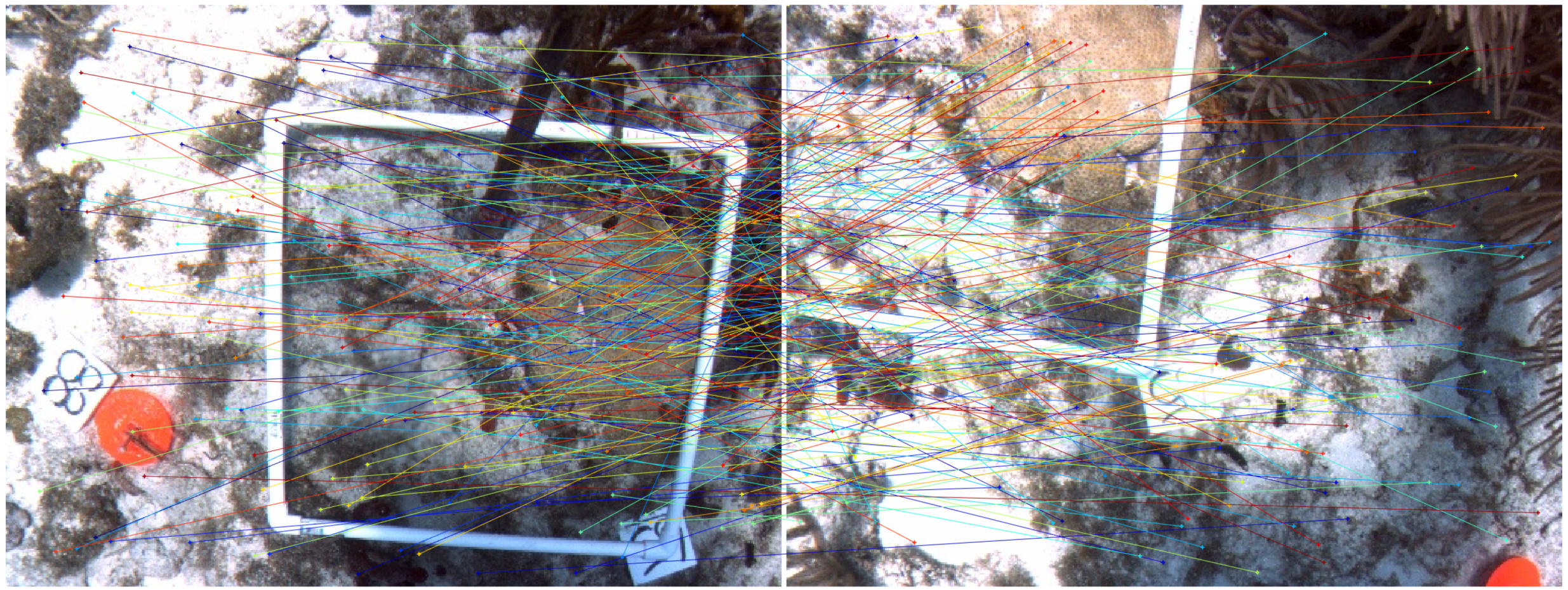
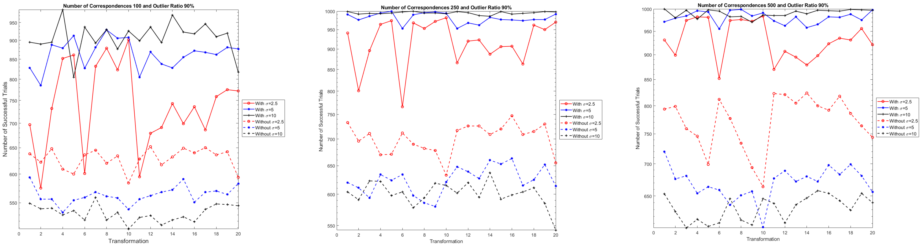
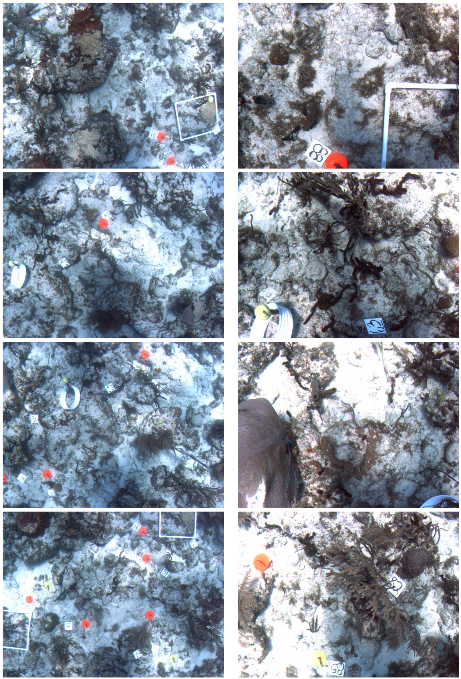
4. Experimental Results
4.1. Experiment 1
| Algorithm 1: Experimental Simulations |
 |
| Algorithm 2: Experimental Simulations |
 |
4.2. Experiment 2
5. Conclusions
Author Contributions
Funding
Acknowledgments
Conflicts of Interest
Abbreviations
| DOF | Degree of Freedom |
| RANSAC | Random Sampling Consensus |
| MSAC | M-estimator Sample Consensus |
| MLESAC | Maximum Likelihood Estimator Sample Consensus |
| PROSAC | Progressive Sample Consensus |
| SIFT | Scale Invariant Feature Transform |
Appendix A. List of Transformations Used in Experiments

| Transformation | (In Rad.) | (In Rad.) | ||
|---|---|---|---|---|
| 1 | 0.89 | 0.88 | −0.24 | 0.97 |
| 2 | 0.74 | 0.73 | −0.69 | −2.51 |
| 3 | 0.54 | 0.53 | −1.39 | −2.45 |
| 4 | 0.43 | 0.42 | 0.15 | −3.06 |
| 5 | 0.39 | 0.33 | −0.71 | −2.88 |
| 6 | 0.82 | 0.82 | −0.55 | −2.36 |
| 7 | 0.57 | 0.52 | 2.62 | −0.25 |
| 8 | 0.41 | 0.40 | −2.09 | −0.61 |
| 9 | 0.33 | 0.33 | −0.40 | 1.85 |
| 10 | 0.26 | 0.23 | 2.68 | 0.10 |
| 11 | 1.01 | 0.87 | −0.27 | 1.13 |
| 12 | 1.07 | 0.82 | 0.34 | 1.33 |
| 13 | 1.22 | 0.61 | −0.47 | 1.28 |
| 14 | 1.20 | 0.60 | 0.09 | 1.29 |
| 15 | 1.23 | 0.60 | 0.66 | 1.43 |
| 16 | 0.92 | 0.79 | −0.02 | 1.63 |
| 17 | 0.90 | 0.67 | −0.04 | 1.66 |
| 18 | 0.88 | 0.55 | −0.05 | 1.67 |
| 19 | 0.87 | 0.41 | −0.09 | 1.68 |
| 20 | 0.91 | 0.26 | −0.11 | 1.68 |
 |  |  |  |
| 1 | 2 | 3 | 4 |
 |  |  |  |
| 5 | 6 | 7 | 8 |
 |  |  |  |
| 9 | 10 | 11 | 12 |
 |  |  |  |
| 13 | 14 | 15 | 16 |
 |  |  |  |
| 17 | 18 | 19 | 20 |
References
- Zitová, B.; Flusser, J. Image registration methods: A survey. Image Vis. Comput. 2003, 21, 977–1000. [Google Scholar] [CrossRef]
- Fischler, M.A.; Bolles, R.C. Random sample consensus: A paradigm for model fitting with applications to image analysis and automated cartography. Commun. ACM 1981, 24, 381–395. [Google Scholar] [CrossRef]
- Hartley, R.; Zisserman, A. Multiple View Geometry in Computer Vision, 2nd ed.; Cambridge University Press: Cambridge, UK, 2004. [Google Scholar]
- Torr, P.; Zisserman, A. MLESAC: A New Robust Estimator with Application to Estimating Image Geometry. Comput. Vis. Image Underst. 2000, 78, 138–156. [Google Scholar] [CrossRef]
- Tordoff, B.J.; Murray, D.W. Guided-MLESAC: Faster Image Transform Estimation by Using Matching Priors. IEEE Trans. Pattern Anal. Mach. Intell. 2005, 27, 1523–1535. [Google Scholar] [CrossRef] [PubMed]
- Chum, O.; Matas, J. Matching with PROSAC. Proc. Comput. Vis. Pattern Recognit. 2005, 1, 220–226. [Google Scholar]
- Raguram, R.; Frahm, J.-M.; Pollefeys, M. A Comparative Analysis of RANSAC Techniques Leading to Adaptive Real-Time Random Sample Consensus. In Computer Vision—ECCV 2008; Lecture Notes in Computer Science; Springer: Berlin/Heidelberg, Germany, 2008; Volume 5303, pp. 500–513. [Google Scholar]
- Senthilnath, J.; Kalro, N.P.; Benediktsson, J.A. Accurate point matching based on multi-objective Genetic Algorithm for multi-sensor satellite imagery. Appl. Math. Comput. 2014, 236, 546–564. [Google Scholar] [CrossRef]
- Le, V.-H.; Vu, H.; Nguyen, T.T.; Le, T.-L.; Tran, T.-H. Acquiring qualified samples for RANSAC using geometrical constraints. Pattern Recognit. Lett. 2018, 102, 58–66. [Google Scholar]
- Marszalek, M.; Rokita, P. Pattern matching with differential voting and median transformation derivation improved point-pattern matching algorithm for two-dimensional coordinate lists. Comput. Imaging Vis. 2006, 32, 1002–1007. [Google Scholar]
- Reiss, T.H. Recognizing Planar Objects Using Invariant Image Features; Lecture Notes in Computer Science; Springer: Berlin/Heidelberg, Germany, 1993; Volume 676. [Google Scholar]
- Byer, O.; Lazebnik, F.; Smeltzer, D.L. Methods for Euclidean Geometry; Mathematical Association of America: Washington, DC, USA, 2010. [Google Scholar]
- Gracias, N.; Negahdaripour, S. Underwater mosaic creation using video sequences from different altitudes. In Proceedings of the OCEANS 2005 MTS/IEEE, Washington, DC, USA, 17–23 September 2005; Volume 2, pp. 1295–1300. [Google Scholar]
- Lowe, D.G. Distinctive image features from scale-invariant keypoints. Int. J. Comput. Vis. 2004, 60, 91–110. [Google Scholar] [CrossRef]
- Datasets from Visual Geometry Group, Department of Engineering Science, University of Oxford. Available online: http://www.robots.ox.ac.uk/~vgg/data/data-aff.html (accessed on 30 November 2018).
- Kovesi, P.D. MATLAB and Octave Functions for Computer Vision and Image Processing. Available online: http://www.peterkovesi.com/matlabfns/ (accessed on 30 November 2018).
- Choukroun, A.; Charvillat, V. Bucketing Techniques in Robust Regression for Computer Vision; Lecture Notes in Computer Science; Springer: Berlin/Heidelberg, Germany, 2003; Volume 2749, pp. 609–616. [Google Scholar]


| Number of Corresp. | Transformation | Outlier Ratio | |||||||||||||||
|---|---|---|---|---|---|---|---|---|---|---|---|---|---|---|---|---|---|
| 75% | 80% | 85% | 90% | ||||||||||||||
| Number of | Average Number of | Number of | Average Number of | Number of | Average Number of | Number of | Average Number of | ||||||||||
| Successful Trials | Iterations in RANSAC | Successful Trials | Iterations in RANSAC | Successful Trials | Iterations in RANSAC | Successful Trials | Iterations in RANSAC | ||||||||||
| without | with | without | with | without | with | without | with | without | with | without | with | without | with | without | with | ||
| 100 | 1 | 1000 | 1000 | 438.87 | 1.09 | 999 | 1000 | 860.18 | 4.19 | 939 | 1000 | 1000 | 22.09 | 631 | 964 | 1000 | 152.89 |
| 2 | 1000 | 1000 | 438.72 | 1.73 | 1000 | 1000 | 860.13 | 6.74 | 932 | 1000 | 1000 | 26.96 | 659 | 954 | 1000 | 176.96 | |
| 3 | 1000 | 1000 | 438.60 | 1.48 | 1000 | 1000 | 859.56 | 6.27 | 943 | 1000 | 1000 | 26.73 | 647 | 960 | 1000 | 156.50 | |
| 4 | 1000 | 1000 | 438.96 | 1.34 | 999 | 1000 | 860.68 | 5.54 | 943 | 1000 | 1000 | 24.92 | 629 | 966 | 1000 | 169.10 | |
| 5 | 1000 | 1000 | 438.77 | 1.52 | 998 | 1000 | 860.82 | 6.19 | 927 | 1000 | 1000 | 26.07 | 631 | 957 | 1000 | 182.35 | |
| 6 | 1000 | 1000 | 438.64 | 1.69 | 999 | 1000 | 860.67 | 6.97 | 938 | 1000 | 1000 | 26.95 | 649 | 949 | 1000 | 173.58 | |
| 7 | 1000 | 1000 | 438.83 | 1.55 | 998 | 1000 | 860.57 | 6.36 | 946 | 1000 | 1000 | 27.62 | 630 | 963 | 1000 | 165.56 | |
| 8 | 1000 | 1000 | 438.61 | 1.41 | 997 | 1000 | 860.49 | 5.91 | 936 | 1000 | 1000 | 26.04 | 615 | 958 | 1000 | 178.13 | |
| 9 | 1000 | 1000 | 438.88 | 2.02 | 999 | 1000 | 859.84 | 7.56 | 931 | 1000 | 1000 | 28.32 | 639 | 951 | 1000 | 180.55 | |
| 10 | 1000 | 1000 | 438.90 | 1.49 | 999 | 1000 | 860.00 | 6.45 | 951 | 1000 | 1000 | 26.00 | 650 | 961 | 1000 | 167.25 | |
| 11 | 1000 | 1000 | 438.71 | 1.63 | 999 | 1000 | 860.78 | 6.63 | 929 | 1000 | 1000 | 25.82 | 632 | 962 | 1000 | 163.30 | |
| 12 | 1000 | 1000 | 438.89 | 1.48 | 999 | 1000 | 860.33 | 6.33 | 941 | 1000 | 1000 | 25.43 | 638 | 966 | 1000 | 162.66 | |
| 13 | 1000 | 1000 | 438.85 | 1.87 | 997 | 1000 | 859.65 | 7.59 | 962 | 1000 | 1000 | 28.39 | 644 | 936 | 1000 | 178.02 | |
| 14 | 1000 | 1000 | 438.90 | 1.91 | 999 | 1000 | 860.88 | 7.49 | 943 | 1000 | 1000 | 28.16 | 643 | 955 | 1000 | 171.39 | |
| 15 | 1000 | 1000 | 438.86 | 1.76 | 999 | 1000 | 860.50 | 7.11 | 943 | 1000 | 1000 | 27.54 | 635 | 955 | 1000 | 175.68 | |
| 16 | 1000 | 1000 | 439.22 | 1.56 | 998 | 1000 | 860.77 | 6.51 | 940 | 1000 | 1000 | 26.79 | 609 | 963 | 1000 | 173.69 | |
| 17 | 1000 | 1000 | 438.84 | 1.41 | 1000 | 1000 | 860.29 | 6.07 | 932 | 1000 | 1000 | 25.42 | 635 | 969 | 1000 | 160.51 | |
| 18 | 1000 | 1000 | 438.81 | 1.51 | 1000 | 1000 | 860.08 | 6.12 | 930 | 1000 | 1000 | 26.26 | 647 | 957 | 1000 | 172.25 | |
| 19 | 1000 | 1000 | 438.83 | 1.73 | 1000 | 1000 | 860.53 | 7.10 | 943 | 1000 | 1000 | 27.62 | 645 | 963 | 1000 | 165.88 | |
| 20 | 1000 | 1000 | 439.06 | 2.78 | 998 | 1000 | 860.72 | 9.28 | 937 | 999 | 1000 | 32.41 | 632 | 945 | 1000 | 184.38 | |
| 250 | 1 | 1000 | 1000 | 429.09 | 1.00 | 999 | 1000 | 859.87 | 1.00 | 968 | 1000 | 1000 | 1.03 | 654 | 1000 | 1000 | 8.54 |
| 2 | 1000 | 1000 | 428.86 | 1.01 | 1000 | 1000 | 860.10 | 1.03 | 971 | 1000 | 1000 | 1.22 | 642 | 1000 | 1000 | 16.78 | |
| 3 | 1000 | 1000 | 428.86 | 1.00 | 1000 | 1000 | 860.33 | 1.01 | 972 | 1000 | 1000 | 1.16 | 629 | 1000 | 1000 | 15.93 | |
| 4 | 1000 | 1000 | 428.81 | 1.00 | 1000 | 1000 | 860.46 | 1.00 | 955 | 1000 | 1000 | 1.10 | 632 | 1000 | 1000 | 13.14 | |
| 5 | 1000 | 1000 | 428.90 | 1.00 | 999 | 1000 | 860.50 | 1.01 | 958 | 1000 | 1000 | 1.19 | 633 | 1000 | 1000 | 17.27 | |
| 6 | 1000 | 1000 | 428.88 | 1.03 | 998 | 1000 | 860.83 | 1.02 | 965 | 1000 | 1000 | 1.22 | 632 | 1000 | 1000 | 19.33 | |
| 7 | 1000 | 1000 | 428.96 | 1.01 | 1000 | 1000 | 860.25 | 1.02 | 962 | 1000 | 1000 | 1.15 | 624 | 999 | 1000 | 17.91 | |
| 8 | 1000 | 1000 | 428.74 | 1.00 | 1000 | 1000 | 860.10 | 1.02 | 952 | 1000 | 1000 | 1.13 | 643 | 1000 | 1000 | 13.64 | |
| 9 | 1000 | 1000 | 428.85 | 1.01 | 999 | 1000 | 860.45 | 1.05 | 964 | 1000 | 1000 | 1.42 | 622 | 1000 | 1000 | 21.92 | |
| 10 | 1000 | 1000 | 428.79 | 1.01 | 999 | 1000 | 860.34 | 1.02 | 958 | 1000 | 1000 | 1.17 | 611 | 1000 | 1000 | 18.21 | |
| 11 | 1000 | 1000 | 428.69 | 1.01 | 1000 | 1000 | 860.13 | 1.02 | 949 | 1000 | 1000 | 1.23 | 665 | 1000 | 1000 | 15.70 | |
| 12 | 1000 | 1000 | 428.62 | 1.00 | 1000 | 1000 | 860.15 | 1.01 | 972 | 1000 | 1000 | 1.12 | 610 | 1000 | 1000 | 14.29 | |
| 13 | 1000 | 1000 | 428.82 | 1.00 | 1000 | 1000 | 860.45 | 1.05 | 960 | 1000 | 1000 | 1.82 | 632 | 1000 | 1000 | 28.41 | |
| 14 | 1000 | 1000 | 428.67 | 1.01 | 1000 | 1000 | 859.85 | 1.02 | 971 | 1000 | 1000 | 1.65 | 647 | 999 | 1000 | 25.02 | |
| 15 | 1000 | 1000 | 428.76 | 1.01 | 1000 | 1000 | 860.30 | 1.03 | 950 | 1000 | 1000 | 1.44 | 636 | 1000 | 1000 | 23.54 | |
| 16 | 1000 | 1000 | 428.80 | 1.00 | 1000 | 1000 | 860.25 | 1.02 | 964 | 1000 | 1000 | 1.18 | 640 | 1000 | 1000 | 14.33 | |
| 17 | 1000 | 1000 | 428.78 | 1.00 | 1000 | 1000 | 860.10 | 1.02 | 961 | 1000 | 1000 | 1.15 | 632 | 1000 | 1000 | 13.39 | |
| 18 | 1000 | 1000 | 428.81 | 1.00 | 999 | 1000 | 860.19 | 1.02 | 970 | 1000 | 1000 | 1.14 | 634 | 1000 | 1000 | 13.53 | |
| 19 | 1000 | 1000 | 428.70 | 1.00 | 1000 | 1000 | 860.01 | 1.03 | 971 | 1000 | 1000 | 1.36 | 660 | 999 | 1000 | 22.09 | |
| 20 | 1000 | 1000 | 428.81 | 1.02 | 1000 | 1000 | 860.35 | 1.10 | 953 | 1000 | 1000 | 3.13 | 653 | 999 | 1000 | 32.08 | |
| 500 | 1 | 1000 | 1000 | 438.68 | 2.79 | 999 | 1000 | 860.26 | 3.34 | 950 | 1000 | 1000 | 5.96 | 643 | 1000 | 1000 | 30.36 |
| 2 | 1000 | 1000 | 438.83 | 2.85 | 999 | 1000 | 860.23 | 3.53 | 965 | 1000 | 1000 | 8.95 | 657 | 1000 | 1000 | 35.72 | |
| 3 | 1000 | 1000 | 438.70 | 2.76 | 1000 | 1000 | 860.09 | 3.52 | 963 | 1000 | 1000 | 8.44 | 652 | 1000 | 1000 | 35.79 | |
| 4 | 1000 | 1000 | 439.00 | 2.82 | 1000 | 1000 | 860.15 | 3.32 | 962 | 1000 | 1000 | 7.21 | 614 | 999 | 1000 | 34.25 | |
| 5 | 1000 | 1000 | 438.88 | 2.87 | 1000 | 1000 | 860.09 | 3.44 | 961 | 1000 | 1000 | 8.23 | 635 | 1000 | 1000 | 38.62 | |
| 6 | 1000 | 1000 | 438.90 | 2.84 | 999 | 1000 | 860.53 | 3.50 | 958 | 1000 | 1000 | 8.70 | 629 | 1000 | 1000 | 38.56 | |
| 7 | 1000 | 1000 | 438.73 | 2.82 | 1000 | 1000 | 860.12 | 3.59 | 969 | 1000 | 1000 | 8.57 | 631 | 1000 | 1000 | 37.47 | |
| 8 | 1000 | 1000 | 438.89 | 2.81 | 1000 | 1000 | 860.09 | 3.43 | 962 | 1000 | 1000 | 8.10 | 667 | 1000 | 1000 | 34.73 | |
| 9 | 1000 | 1000 | 438.75 | 2.81 | 1000 | 1000 | 860.04 | 3.65 | 957 | 1000 | 1000 | 9.53 | 634 | 1000 | 1000 | 39.19 | |
| 10 | 1000 | 1000 | 439.13 | 2.76 | 1000 | 1000 | 860.41 | 3.51 | 965 | 1000 | 1000 | 8.72 | 629 | 1000 | 1000 | 36.94 | |
| 11 | 1000 | 1000 | 438.68 | 2.80 | 1000 | 1000 | 860.04 | 3.46 | 960 | 1000 | 1000 | 8.54 | 630 | 1000 | 1000 | 36.04 | |
| 12 | 1000 | 1000 | 438.79 | 2.75 | 1000 | 1000 | 860.50 | 3.47 | 961 | 1000 | 1000 | 7.94 | 620 | 1000 | 1000 | 35.04 | |
| 13 | 1000 | 1000 | 438.60 | 2.81 | 1000 | 1000 | 860.26 | 3.61 | 953 | 1000 | 1000 | 9.62 | 641 | 1000 | 1000 | 39.41 | |
| 14 | 1000 | 1000 | 438.81 | 2.83 | 1000 | 1000 | 860.22 | 3.60 | 949 | 1000 | 1000 | 9.86 | 647 | 1000 | 1000 | 39.41 | |
| 15 | 1000 | 1000 | 438.73 | 2.78 | 1000 | 1000 | 860.28 | 3.56 | 955 | 1000 | 1000 | 9.26 | 626 | 1000 | 1000 | 37.94 | |
| 16 | 1000 | 1000 | 438.62 | 2.81 | 1000 | 1000 | 860.25 | 3.43 | 963 | 1000 | 1000 | 8.04 | 635 | 1000 | 1000 | 34.24 | |
| 17 | 1000 | 1000 | 438.73 | 2.83 | 999 | 1000 | 860.49 | 3.46 | 968 | 1000 | 1000 | 7.47 | 654 | 1000 | 1000 | 33.28 | |
| 18 | 1000 | 1000 | 438.72 | 2.74 | 999 | 1000 | 860.44 | 3.50 | 964 | 1000 | 1000 | 7.36 | 636 | 1000 | 1000 | 34.14 | |
| 19 | 1000 | 1000 | 438.79 | 2.80 | 999 | 1000 | 859.89 | 3.58 | 959 | 1000 | 1000 | 9.03 | 633 | 1000 | 1000 | 37.85 | |
| 20 | 1000 | 1000 | 438.77 | 2.85 | 999 | 1000 | 860.34 | 4.11 | 965 | 1000 | 1000 | 12.90 | 634 | 1000 | 1000 | 41.79 | |
| Number of Corresp. | Noise | Transformation | Outlier Ratio | |||||||||||||||
|---|---|---|---|---|---|---|---|---|---|---|---|---|---|---|---|---|---|---|
| 75% | 80% | 85% | 90% | |||||||||||||||
| Number of | Average Number of | Number of | Average Number of | Number of | Average Number of | Number of | Average Number of | |||||||||||
| Successful Trials | Iterations in RANSAC | Successful Trials | Iterations in RANSAC | Successful Trials | Iterations in RANSAC | Successful Trials | Iterations in RANSAC | |||||||||||
| without | with | without | with | without | with | without | with | without | with | without | with | without | with | without | with | |||
| 100 | 2.5 | 1 | 1000 | 1000 | 422.38 | 17.12 | 1000 | 998 | 822.24 | 22.25 | 973 | 979 | 1000 | 66.44 | 638 | 697 | 1000 | 247.77 |
| 2 | 1000 | 1000 | 427.47 | 26.68 | 998 | 1000 | 824.89 | 45.24 | 966 | 990 | 1000 | 75.14 | 622 | 575 | 1000 | 403.28 | ||
| 3 | 1000 | 1000 | 430.38 | 15.48 | 1000 | 1000 | 839.92 | 31.65 | 952 | 997 | 1000 | 54.92 | 648 | 732 | 1000 | 331.70 | ||
| 4 | 1000 | 1000 | 432.22 | 13.46 | 1000 | 1000 | 844.44 | 24.24 | 961 | 998 | 1000 | 50.04 | 609 | 852 | 1000 | 262.85 | ||
| 5 | 1000 | 1000 | 434.62 | 14.17 | 999 | 1000 | 847.44 | 23.59 | 963 | 998 | 1000 | 51.14 | 600 | 861 | 1000 | 281.51 | ||
| 6 | 1000 | 998 | 424.53 | 26.90 | 1000 | 990 | 825.58 | 48.63 | 957 | 953 | 1000 | 134.35 | 636 | 601 | 1000 | 365.58 | ||
| 7 | 1000 | 1000 | 430.12 | 15.80 | 1000 | 999 | 835.41 | 34.53 | 960 | 995 | 1000 | 65.38 | 645 | 832 | 1000 | 245.39 | ||
| 8 | 1000 | 1000 | 433.27 | 17.51 | 1000 | 1000 | 845.14 | 21.94 | 953 | 1000 | 1000 | 49.53 | 620 | 879 | 1000 | 269.25 | ||
| 9 | 1000 | 1000 | 434.17 | 16.24 | 1000 | 1000 | 848.40 | 26.46 | 965 | 1000 | 1000 | 44.74 | 634 | 823 | 1000 | 318.33 | ||
| 10 | 1000 | 1000 | 436.62 | 11.60 | 999 | 1000 | 854.00 | 22.50 | 961 | 1000 | 1000 | 36.90 | 584 | 902 | 1000 | 286.92 | ||
| 11 | 1000 | 1000 | 422.47 | 26.58 | 999 | 992 | 815.03 | 40.11 | 969 | 953 | 1000 | 103.61 | 628 | 595 | 999 | 353.94 | ||
| 12 | 1000 | 1000 | 422.35 | 20.47 | 1000 | 994 | 813.67 | 47.30 | 966 | 964 | 1000 | 98.23 | 652 | 679 | 1000 | 283.07 | ||
| 13 | 1000 | 999 | 423.85 | 25.81 | 999 | 1000 | 824.05 | 43.80 | 964 | 979 | 1000 | 109.86 | 617 | 691 | 1000 | 368.18 | ||
| 14 | 1000 | 1000 | 425.23 | 21.80 | 999 | 998 | 824.60 | 40.44 | 969 | 970 | 1000 | 117.16 | 632 | 743 | 1000 | 328.18 | ||
| 15 | 1000 | 1000 | 424.09 | 28.28 | 1000 | 997 | 826.24 | 50.82 | 967 | 966 | 1000 | 111.34 | 649 | 699 | 1000 | 364.10 | ||
| 16 | 1000 | 1000 | 423.53 | 23.23 | 999 | 995 | 825.22 | 38.66 | 960 | 963 | 1000 | 94.46 | 640 | 736 | 999 | 280.46 | ||
| 17 | 1000 | 999 | 425.46 | 21.62 | 1000 | 996 | 828.31 | 31.28 | 966 | 984 | 1000 | 82.94 | 650 | 686 | 1000 | 294.11 | ||
| 18 | 1000 | 999 | 426.26 | 18.53 | 1000 | 1000 | 831.02 | 31.60 | 978 | 979 | 1000 | 83.28 | 636 | 759 | 1000 | 299.63 | ||
| 19 | 1000 | 1000 | 429.59 | 20.74 | 999 | 1000 | 835.25 | 35.59 | 970 | 990 | 1000 | 71.29 | 642 | 775 | 1000 | 336.23 | ||
| 20 | 1000 | 1000 | 432.04 | 20.80 | 1000 | 1000 | 843.39 | 31.85 | 964 | 996 | 1000 | 82.86 | 594 | 772 | 1000 | 438.50 | ||
| 100 | 5 | 1 | 1000 | 1000 | 434.59 | 9.24 | 999 | 999 | 850.68 | 19.81 | 945 | 1000 | 1000 | 40.58 | 594 | 828 | 999 | 286.74 |
| 2 | 1000 | 1000 | 435.73 | 16.67 | 999 | 1000 | 852.04 | 26.87 | 949 | 1000 | 1000 | 60.01 | 556 | 785 | 999 | 342.96 | ||
| 3 | 1000 | 1000 | 436.75 | 12.13 | 1000 | 1000 | 854.93 | 20.63 | 940 | 1000 | 1000 | 52.16 | 556 | 888 | 1000 | 272.93 | ||
| 4 | 1000 | 1000 | 437.33 | 11.00 | 1000 | 1000 | 857.50 | 17.41 | 957 | 1000 | 1000 | 38.96 | 534 | 879 | 1000 | 303.93 | ||
| 5 | 1000 | 1000 | 438.09 | 9.94 | 1000 | 1000 | 858.35 | 18.96 | 956 | 1000 | 1000 | 40.14 | 554 | 913 | 1000 | 288.07 | ||
| 6 | 1000 | 999 | 435.23 | 14.62 | 1000 | 999 | 853.42 | 28.07 | 949 | 995 | 1000 | 68.56 | 559 | 827 | 1000 | 304.31 | ||
| 7 | 1000 | 1000 | 436.66 | 12.62 | 1000 | 1000 | 853.73 | 22.03 | 951 | 998 | 1000 | 48.92 | 568 | 881 | 1000 | 285.86 | ||
| 8 | 1000 | 1000 | 437.73 | 11.49 | 1000 | 1000 | 857.93 | 18.35 | 936 | 1000 | 1000 | 38.41 | 561 | 929 | 1000 | 233.94 | ||
| 9 | 1000 | 1000 | 437.83 | 12.62 | 998 | 1000 | 858.48 | 21.28 | 949 | 999 | 1000 | 42.14 | 558 | 906 | 1000 | 281.63 | ||
| 10 | 1000 | 1000 | 438.31 | 9.17 | 1000 | 1000 | 859.51 | 18.78 | 947 | 1000 | 1000 | 37.64 | 539 | 908 | 1000 | 262.63 | ||
| 11 | 1000 | 1000 | 434.53 | 15.93 | 1000 | 1000 | 850.21 | 27.40 | 942 | 997 | 1000 | 58.08 | 556 | 805 | 1000 | 315.21 | ||
| 12 | 1000 | 1000 | 434.91 | 14.62 | 997 | 999 | 851.59 | 27.66 | 960 | 991 | 1000 | 61.29 | 562 | 869 | 1000 | 270.01 | ||
| 13 | 1000 | 1000 | 435.16 | 17.53 | 999 | 1000 | 851.54 | 31.34 | 946 | 999 | 1000 | 63.62 | 568 | 838 | 1000 | 358.61 | ||
| 14 | 1000 | 1000 | 435.37 | 17.86 | 999 | 1000 | 852.95 | 25.48 | 939 | 1000 | 1000 | 58.41 | 572 | 828 | 1000 | 356.95 | ||
| 15 | 1000 | 1000 | 434.58 | 19.03 | 999 | 1000 | 850.59 | 29.86 | 949 | 995 | 1000 | 72.93 | 591 | 855 | 1000 | 325.13 | ||
| 16 | 1000 | 1000 | 435.41 | 16.71 | 998 | 1000 | 851.03 | 24.07 | 955 | 996 | 1000 | 56.25 | 551 | 872 | 1000 | 258.49 | ||
| 17 | 1000 | 1000 | 435.76 | 15.41 | 1000 | 1000 | 853.31 | 25.86 | 954 | 1000 | 1000 | 54.36 | 568 | 868 | 1000 | 259.37 | ||
| 18 | 1000 | 1000 | 436.06 | 13.21 | 1000 | 1000 | 854.21 | 21.20 | 950 | 998 | 1000 | 59.14 | 570 | 862 | 1000 | 297.56 | ||
| 19 | 1000 | 1000 | 437.17 | 13.34 | 1000 | 1000 | 853.18 | 23.59 | 950 | 1000 | 1000 | 44.79 | 564 | 881 | 1000 | 306.86 | ||
| 20 | 1000 | 1000 | 437.97 | 15.31 | 1000 | 1000 | 856.75 | 28.14 | 942 | 1000 | 1000 | 51.78 | 583 | 877 | 1000 | 390.24 | ||
| 100 | 10 | 1 | 1000 | 1000 | 438.25 | 8.76 | 999 | 1000 | 858.73 | 19.29 | 940 | 1000 | 1000 | 35.93 | 549 | 895 | 1000 | 277.67 |
| 2 | 1000 | 1000 | 438.65 | 12.09 | 1000 | 1000 | 859.00 | 22.09 | 949 | 1000 | 1000 | 37.03 | 540 | 890 | 1000 | 299.06 | ||
| 3 | 1000 | 1000 | 438.41 | 9.75 | 1000 | 1000 | 859.70 | 17.45 | 937 | 1000 | 1000 | 40.06 | 541 | 895 | 999 | 325.11 | ||
| 4 | 1000 | 1000 | 438.39 | 8.03 | 1000 | 1000 | 860.09 | 15.71 | 949 | 1000 | 1000 | 36.14 | 530 | 988 | 1000 | 101.85 | ||
| 5 | 1000 | 1000 | 438.52 | 6.90 | 1000 | 1000 | 860.27 | 14.94 | 937 | 1000 | 1000 | 37.63 | 537 | 805 | 1000 | 423.70 | ||
| 6 | 1000 | 1000 | 438.37 | 12.89 | 999 | 1000 | 859.49 | 22.05 | 956 | 1000 | 1000 | 36.71 | 522 | 937 | 1000 | 198.73 | ||
| 7 | 1000 | 1000 | 439.22 | 9.08 | 999 | 1000 | 859.61 | 19.64 | 935 | 1000 | 1000 | 36.97 | 559 | 893 | 1000 | 308.48 | ||
| 8 | 1000 | 1000 | 438.85 | 6.67 | 1000 | 1000 | 859.79 | 17.87 | 943 | 1000 | 1000 | 36.00 | 522 | 930 | 1000 | 255.70 | ||
| 9 | 1000 | 1000 | 438.66 | 9.24 | 1000 | 1000 | 860.50 | 20.30 | 948 | 1000 | 1000 | 37.63 | 534 | 877 | 1000 | 328.77 | ||
| 10 | 1000 | 1000 | 439.06 | 6.91 | 1000 | 1000 | 860.35 | 15.48 | 943 | 1000 | 1000 | 34.40 | 508 | 926 | 1000 | 249.76 | ||
| 11 | 1000 | 1000 | 438.12 | 11.08 | 998 | 1000 | 859.15 | 21.56 | 950 | 1000 | 1000 | 46.94 | 526 | 899 | 1000 | 283.15 | ||
| 12 | 1000 | 1000 | 437.84 | 13.51 | 1000 | 1000 | 856.90 | 19.14 | 949 | 1000 | 1000 | 39.72 | 529 | 937 | 1000 | 240.97 | ||
| 13 | 1000 | 1000 | 438.60 | 11.10 | 999 | 1000 | 858.78 | 20.63 | 947 | 1000 | 1000 | 42.65 | 514 | 894 | 999 | 314.33 | ||
| 14 | 1000 | 1000 | 438.12 | 12.28 | 998 | 1000 | 859.39 | 21.90 | 939 | 1000 | 1000 | 40.07 | 522 | 972 | 1000 | 179.03 | ||
| 15 | 1000 | 1000 | 438.06 | 11.84 | 1000 | 1000 | 857.70 | 21.95 | 935 | 1000 | 1000 | 39.19 | 527 | 923 | 1000 | 271.82 | ||
| 16 | 1000 | 1000 | 438.12 | 11.18 | 999 | 1000 | 858.92 | 22.29 | 951 | 1000 | 1000 | 38.02 | 519 | 918 | 1000 | 277.09 | ||
| 17 | 1000 | 1000 | 438.31 | 12.03 | 1000 | 1000 | 859.14 | 20.45 | 942 | 1000 | 1000 | 40.12 | 539 | 946 | 1000 | 225.12 | ||
| 18 | 1000 | 1000 | 438.00 | 10.32 | 999 | 1000 | 858.27 | 19.62 | 943 | 1000 | 1000 | 39.50 | 548 | 910 | 1000 | 277.68 | ||
| 19 | 1000 | 1000 | 438.82 | 10.24 | 999 | 1000 | 859.80 | 21.59 | 954 | 1000 | 1000 | 36.81 | 547 | 920 | 1000 | 280.26 | ||
| 20 | 1000 | 1000 | 438.71 | 10.74 | 1000 | 1000 | 860.16 | 19.79 | 933 | 1000 | 1000 | 39.29 | 545 | 817 | 1000 | 449.70 | ||
| Number of Corresp. | Noise | Transformation | Outlier Ratio | |||||||||||||||
|---|---|---|---|---|---|---|---|---|---|---|---|---|---|---|---|---|---|---|
| 75% | 80% | 85% | 90% | |||||||||||||||
| Number of | Average Number of | Number of | Average Number of | Number of | Average Number of | Number of | Average Number of | |||||||||||
| Successful Trials | Iterations in RANSAC | Successful Trials | Iterations in RANSAC | Successful Trials | Iterations in RANSAC | Successful Trials | Iterations in RANSAC | |||||||||||
| without | with | without | with | without | with | without | with | without | with | without | with | without | with | without | with | |||
| 250 | 2.5 | 1 | 1000 | 1000 | 433.28 | 7.73 | 1000 | 1000 | 819.85 | 12.78 | 983 | 994 | 1000 | 32.14 | 733 | 941 | 1000 | 86.58 |
| 2 | 1000 | 997 | 435.94 | 32.31 | 1000 | 998 | 824.42 | 37.53 | 978 | 982 | 1000 | 69.99 | 696 | 801 | 1000 | 267.96 | ||
| 3 | 1000 | 1000 | 440.31 | 10.15 | 999 | 1000 | 837.23 | 15.05 | 970 | 998 | 1000 | 29.51 | 711 | 896 | 1000 | 154.72 | ||
| 4 | 1000 | 1000 | 442.37 | 8.22 | 999 | 1000 | 844.88 | 12.33 | 978 | 1000 | 1000 | 24.63 | 670 | 964 | 1000 | 113.48 | ||
| 5 | 1000 | 1000 | 444.53 | 6.40 | 998 | 1000 | 847.38 | 11.59 | 968 | 1000 | 1000 | 18.90 | 671 | 974 | 1000 | 112.26 | ||
| 6 | 1000 | 1000 | 433.31 | 36.66 | 999 | 998 | 822.78 | 59.31 | 969 | 956 | 1000 | 125.89 | 712 | 766 | 1000 | 305.23 | ||
| 7 | 1000 | 1000 | 440.80 | 9.28 | 1000 | 1000 | 836.15 | 15.18 | 979 | 998 | 1000 | 28.18 | 690 | 968 | 1000 | 101.58 | ||
| 8 | 1000 | 1000 | 443.20 | 8.26 | 1000 | 1000 | 844.56 | 12.82 | 963 | 1000 | 1000 | 23.14 | 682 | 953 | 1000 | 130.63 | ||
| 9 | 1000 | 1000 | 444.99 | 10.60 | 1000 | 1000 | 848.88 | 15.65 | 970 | 999 | 1000 | 31.74 | 678 | 972 | 1000 | 115.78 | ||
| 10 | 1000 | 1000 | 446.77 | 5.47 | 1000 | 1000 | 853.80 | 8.71 | 957 | 1000 | 1000 | 20.62 | 633 | 982 | 1000 | 109.07 | ||
| 11 | 1000 | 1000 | 432.11 | 13.37 | 1000 | 998 | 816.18 | 20.74 | 985 | 992 | 1000 | 52.45 | 717 | 866 | 1000 | 152.35 | ||
| 12 | 1000 | 1000 | 432.17 | 11.18 | 1000 | 1000 | 816.97 | 19.86 | 985 | 991 | 1000 | 37.95 | 726 | 920 | 1000 | 111.43 | ||
| 13 | 1000 | 1000 | 432.93 | 11.03 | 1000 | 1000 | 818.91 | 24.94 | 984 | 992 | 1000 | 55.25 | 726 | 923 | 1000 | 171.26 | ||
| 14 | 1000 | 1000 | 434.90 | 18.87 | 1000 | 998 | 821.12 | 20.56 | 983 | 991 | 1000 | 47.00 | 709 | 887 | 1000 | 185.86 | ||
| 15 | 1000 | 1000 | 435.20 | 13.29 | 1000 | 1000 | 821.99 | 27.17 | 992 | 993 | 1000 | 47.11 | 720 | 906 | 1000 | 179.29 | ||
| 16 | 1000 | 1000 | 433.88 | 11.84 | 1000 | 1000 | 819.17 | 17.55 | 979 | 992 | 1000 | 43.37 | 747 | 907 | 1000 | 137.29 | ||
| 17 | 1000 | 999 | 435.12 | 11.64 | 1000 | 1000 | 825.55 | 18.50 | 984 | 995 | 1000 | 43.38 | 709 | 863 | 1000 | 161.55 | ||
| 18 | 1000 | 1000 | 437.65 | 10.33 | 1000 | 999 | 829.66 | 15.99 | 975 | 994 | 1000 | 31.88 | 715 | 962 | 1000 | 103.18 | ||
| 19 | 1000 | 1000 | 440.25 | 11.88 | 1000 | 999 | 834.00 | 15.45 | 981 | 1000 | 1000 | 34.77 | 730 | 950 | 1000 | 124.94 | ||
| 20 | 1000 | 1000 | 442.36 | 10.05 | 1000 | 1000 | 840.73 | 20.81 | 977 | 999 | 1000 | 36.88 | 655 | 970 | 1000 | 145.78 | ||
| 250 | 5 | 1 | 1000 | 1000 | 446.02 | 5.62 | 1000 | 1000 | 850.43 | 8.983 | 962 | 998 | 1000 | 15.56 | 620 | 991 | 1000 | 66.05 |
| 2 | 1000 | 1000 | 446.76 | 8.88 | 1000 | 1000 | 853.51 | 16.215 | 969 | 1000 | 1000 | 25.50 | 611 | 976 | 1000 | 119.56 | ||
| 3 | 1000 | 1000 | 447.96 | 5.79 | 1000 | 1000 | 855.34 | 9.192 | 960 | 1000 | 1000 | 19.73 | 594 | 986 | 1000 | 77.27 | ||
| 4 | 1000 | 1000 | 448.23 | 4.52 | 1000 | 1000 | 856.72 | 6.996 | 952 | 1000 | 1000 | 15.21 | 634 | 995 | 1000 | 81.61 | ||
| 5 | 1000 | 1000 | 448.78 | 4.15 | 1000 | 1000 | 857.39 | 6.413 | 968 | 1000 | 1000 | 14.64 | 624 | 1000 | 1000 | 55.80 | ||
| 6 | 1000 | 1000 | 445.89 | 14.11 | 1000 | 1000 | 851.11 | 19.352 | 967 | 1000 | 1000 | 35.50 | 634 | 953 | 1000 | 161.34 | ||
| 7 | 1000 | 1000 | 447.80 | 5.64 | 999 | 1000 | 854.32 | 9.014 | 952 | 1000 | 1000 | 16.34 | 598 | 990 | 1000 | 74.82 | ||
| 8 | 1000 | 1000 | 448.36 | 4.48 | 1000 | 1000 | 857.26 | 7.388 | 968 | 1000 | 1000 | 13.89 | 586 | 996 | 1000 | 54.56 | ||
| 9 | 1000 | 1000 | 448.78 | 5.72 | 1000 | 1000 | 858.02 | 10.126 | 949 | 1000 | 1000 | 15.22 | 580 | 998 | 1000 | 65.13 | ||
| 10 | 1000 | 1000 | 449.21 | 2.60 | 1000 | 1000 | 858.85 | 5.584 | 954 | 1000 | 1000 | 12.99 | 621 | 994 | 1000 | 72.94 | ||
| 11 | 1000 | 1000 | 445.52 | 10.20 | 1000 | 1000 | 848.65 | 12.948 | 967 | 998 | 1000 | 24.80 | 648 | 953 | 1000 | 129.81 | ||
| 12 | 1000 | 1000 | 445.22 | 7.81 | 1000 | 1000 | 848.99 | 13.473 | 971 | 999 | 1000 | 26.42 | 639 | 968 | 1000 | 111.93 | ||
| 13 | 1000 | 1000 | 446.30 | 10.47 | 1000 | 1000 | 850.77 | 17.686 | 974 | 999 | 1000 | 35.46 | 627 | 962 | 1000 | 164.56 | ||
| 14 | 1000 | 1000 | 446.30 | 8.96 | 999 | 1000 | 850.11 | 14.528 | 959 | 999 | 1000 | 29.74 | 660 | 983 | 1000 | 122.98 | ||
| 15 | 1000 | 1000 | 446.04 | 7.99 | 1000 | 1000 | 852.35 | 15.486 | 977 | 998 | 1000 | 28.23 | 653 | 977 | 1000 | 116.60 | ||
| 16 | 1000 | 1000 | 445.77 | 8.10 | 999 | 1000 | 850.49 | 13.961 | 962 | 1000 | 1000 | 27.57 | 663 | 976 | 1000 | 105.22 | ||
| 17 | 1000 | 1000 | 445.95 | 7.75 | 999 | 1000 | 853.24 | 11.681 | 958 | 1000 | 1000 | 20.57 | 615 | 974 | 1000 | 93.35 | ||
| 18 | 1000 | 1000 | 446.97 | 7.37 | 1000 | 1000 | 852.21 | 11.06 | 963 | 1000 | 1000 | 20.70 | 625 | 977 | 1000 | 113.94 | ||
| 19 | 1000 | 1000 | 447.65 | 7.08 | 1000 | 1000 | 854.52 | 12.457 | 960 | 1000 | 1000 | 21.00 | 652 | 977 | 1000 | 113.21 | ||
| 20 | 1000 | 1000 | 448.11 | 8.35 | 999 | 1000 | 857.03 | 12.463 | 951 | 1000 | 1000 | 25.87 | 614 | 992 | 1000 | 100.31 | ||
| 250 | 10 | 1 | 1000 | 1000 | 449.12 | 3.11 | 999 | 1000 | 858.17 | 5.36 | 960 | 1000 | 1000 | 12.62 | 604 | 999 | 1000 | 50.60 |
| 2 | 1000 | 1000 | 449.08 | 5.05 | 999 | 1000 | 858.84 | 8.75 | 965 | 1000 | 1000 | 16.60 | 591 | 992 | 1000 | 75.63 | ||
| 3 | 1000 | 1000 | 449.52 | 2.96 | 998 | 1000 | 859.58 | 5.58 | 955 | 1000 | 1000 | 13.35 | 623 | 994 | 1000 | 58.33 | ||
| 4 | 1000 | 1000 | 449.74 | 2.08 | 998 | 1000 | 860.16 | 3.86 | 956 | 1000 | 1000 | 9.17 | 622 | 993 | 1000 | 93.89 | ||
| 5 | 1000 | 1000 | 449.65 | 1.77 | 1000 | 1000 | 859.80 | 3.67 | 958 | 1000 | 1000 | 10.32 | 598 | 995 | 1000 | 90.75 | ||
| 6 | 1000 | 1000 | 449.58 | 5.86 | 999 | 1000 | 858.52 | 9.79 | 955 | 1000 | 1000 | 21.17 | 604 | 998 | 1000 | 57.01 | ||
| 7 | 1000 | 1000 | 449.37 | 3.04 | 1000 | 1000 | 859.70 | 5.53 | 959 | 1000 | 1000 | 12.81 | 578 | 1000 | 1000 | 41.49 | ||
| 8 | 1000 | 1000 | 449.56 | 1.94 | 1000 | 1000 | 859.85 | 3.85 | 954 | 1000 | 1000 | 9.46 | 594 | 995 | 1000 | 78.09 | ||
| 9 | 1000 | 1000 | 449.66 | 2.41 | 999 | 1000 | 860.26 | 4.78 | 942 | 1000 | 1000 | 11.86 | 619 | 995 | 1000 | 53.26 | ||
| 10 | 1000 | 1000 | 450.09 | 1.31 | 1000 | 1000 | 860.60 | 2.42 | 962 | 1000 | 1000 | 8.14 | 615 | 993 | 1000 | 92.71 | ||
| 11 | 1000 | 1000 | 449.14 | 5.84 | 1000 | 1000 | 858.21 | 9.68 | 965 | 1000 | 1000 | 15.63 | 602 | 999 | 1000 | 50.76 | ||
| 12 | 1000 | 1000 | 449.17 | 5.57 | 1000 | 1000 | 857.86 | 9.08 | 955 | 1000 | 1000 | 16.88 | 620 | 996 | 1000 | 68.86 | ||
| 13 | 1000 | 1000 | 449.04 | 5.90 | 1000 | 1000 | 858.30 | 11.06 | 959 | 1000 | 1000 | 19.49 | 595 | 988 | 1000 | 117.74 | ||
| 14 | 1000 | 1000 | 449.26 | 6.13 | 1000 | 1000 | 858.49 | 10.95 | 954 | 1000 | 1000 | 18.51 | 637 | 986 | 1000 | 123.33 | ||
| 15 | 1000 | 1000 | 448.80 | 5.37 | 998 | 1000 | 858.77 | 9.77 | 957 | 1000 | 1000 | 21.27 | 592 | 999 | 1000 | 54.57 | ||
| 16 | 1000 | 1000 | 449.27 | 4.10 | 1000 | 1000 | 858.49 | 8.17 | 960 | 1000 | 1000 | 15.94 | 599 | 992 | 1000 | 80.88 | ||
| 17 | 1000 | 1000 | 449.08 | 4.02 | 1000 | 1000 | 858.20 | 7.50 | 956 | 1000 | 1000 | 15.94 | 604 | 994 | 1000 | 77.48 | ||
| 18 | 1000 | 1000 | 449.31 | 4.04 | 1000 | 1000 | 858.70 | 7.69 | 959 | 1000 | 1000 | 15.51 | 611 | 996 | 1000 | 71.31 | ||
| 19 | 1000 | 1000 | 449.56 | 3.96 | 998 | 1000 | 859.78 | 6.54 | 957 | 1000 | 1000 | 15.68 | 585 | 999 | 1000 | 62.72 | ||
| 20 | 1000 | 1000 | 449.54 | 4.07 | 999 | 1000 | 859.79 | 7.55 | 945 | 1000 | 1000 | 16.71 | 543 | 998 | 1000 | 44.11 | ||
| Number of Corresp. | Noise | Transformation | Outlier Ratio | |||||||||||||||
|---|---|---|---|---|---|---|---|---|---|---|---|---|---|---|---|---|---|---|
| 75% | 80% | 85% | 90% | |||||||||||||||
| Number of | Average Number of | Number of | Average Number of | Number of | Average Number of | Number of | Average Number of | |||||||||||
| Successful Trials | Iterations in RANSAC | Successful Trials | Iterations in RANSAC | Successful Trials | Iterations in RANSAC | Successful Trials | Iterations in RANSAC | |||||||||||
| without | with | without | with | without | with | without | with | without | with | without | with | without | with | without | with | |||
| 500 | 2.5 | 1 | 1000 | 999 | 423.79 | 11.58 | 1000 | 1000 | 816.46 | 15.84 | 994 | 996 | 1000 | 30.47 | 794 | 931 | 1000 | 119.65 |
| 2 | 1000 | 1000 | 425.48 | 18.04 | 1000 | 1000 | 824.93 | 28.88 | 995 | 992 | 1000 | 59.54 | 799 | 899 | 1000 | 202.91 | ||
| 3 | 1000 | 1000 | 430.17 | 11.75 | 1000 | 1000 | 836.86 | 23.05 | 991 | 999 | 1000 | 28.79 | 759 | 974 | 1000 | 112.30 | ||
| 4 | 1000 | 1000 | 432.21 | 10.94 | 999 | 1000 | 843.61 | 14.80 | 984 | 1000 | 1000 | 28.14 | 746 | 982 | 1000 | 101.92 | ||
| 5 | 1000 | 1000 | 433.70 | 8.66 | 1000 | 1000 | 846.70 | 17.75 | 978 | 999 | 1000 | 29.09 | 699 | 981 | 1000 | 87.64 | ||
| 6 | 1000 | 999 | 423.46 | 25.10 | 1000 | 998 | 821.96 | 39.43 | 996 | 990 | 1000 | 66.67 | 812 | 852 | 1000 | 222.88 | ||
| 7 | 1000 | 1000 | 430.42 | 12.41 | 1000 | 1000 | 837.60 | 17.33 | 990 | 999 | 1000 | 29.88 | 777 | 974 | 1000 | 124.03 | ||
| 8 | 1000 | 1000 | 433.19 | 11.36 | 1000 | 1000 | 843.51 | 15.25 | 986 | 1000 | 1000 | 30.49 | 734 | 976 | 1000 | 107.25 | ||
| 9 | 1000 | 1000 | 434.39 | 12.84 | 1000 | 1000 | 848.51 | 18.13 | 985 | 1000 | 1000 | 32.57 | 694 | 972 | 1000 | 125.78 | ||
| 10 | 1000 | 1000 | 436.36 | 7.01 | 1000 | 1000 | 853.78 | 12.93 | 976 | 1000 | 1000 | 18.81 | 664 | 984 | 1000 | 114.13 | ||
| 11 | 1000 | 999 | 421.46 | 14.13 | 1000 | 999 | 815.82 | 26.83 | 992 | 994 | 1000 | 45.39 | 823 | 870 | 1000 | 157.58 | ||
| 12 | 1000 | 1000 | 421.61 | 11.82 | 1000 | 997 | 815.72 | 20.49 | 998 | 991 | 1000 | 49.12 | 821 | 907 | 1000 | 141.68 | ||
| 13 | 1000 | 999 | 423.54 | 18.67 | 1000 | 993 | 822.36 | 30.44 | 996 | 981 | 1000 | 64.86 | 805 | 895 | 1000 | 151.15 | ||
| 14 | 1000 | 1000 | 424.02 | 17.39 | 1000 | 1000 | 819.90 | 30.34 | 990 | 989 | 1000 | 59.79 | 824 | 879 | 1000 | 182.19 | ||
| 15 | 1000 | 1000 | 424.60 | 15.58 | 1000 | 999 | 821.47 | 27.16 | 993 | 994 | 1000 | 46.53 | 800 | 898 | 1000 | 187.97 | ||
| 16 | 1000 | 1000 | 423.42 | 14.89 | 1000 | 996 | 818.55 | 24.88 | 994 | 991 | 1000 | 43.72 | 792 | 923 | 1000 | 143.92 | ||
| 17 | 1000 | 1000 | 425.17 | 11.68 | 1000 | 999 | 823.24 | 23.64 | 985 | 996 | 1000 | 42.86 | 818 | 935 | 1000 | 130.19 | ||
| 18 | 1000 | 1000 | 426.42 | 14.04 | 1000 | 1000 | 828.49 | 20.46 | 994 | 998 | 1000 | 33.29 | 786 | 931 | 1000 | 129.03 | ||
| 19 | 1000 | 1000 | 429.28 | 14.14 | 1000 | 1000 | 832.88 | 21.06 | 991 | 999 | 1000 | 37.41 | 764 | 956 | 1000 | 135.25 | ||
| 20 | 1000 | 1000 | 431.89 | 15.06 | 1000 | 999 | 842.12 | 21.52 | 983 | 998 | 1000 | 38.55 | 744 | 921 | 1000 | 233.27 | ||
| 500 | 5 | 1 | 1000 | 1000 | 434.93 | 7.78 | 1000 | 1000 | 850.33 | 13.99 | 981 | 1000 | 1000 | 24.37 | 720 | 971 | 1000 | 120.87 |
| 2 | 1000 | 1000 | 435.99 | 10.93 | 1000 | 1000 | 851.88 | 19.45 | 967 | 1000 | 1000 | 27.31 | 676 | 979 | 1000 | 97.61 | ||
| 3 | 1000 | 1000 | 436.62 | 7.51 | 1000 | 1000 | 855.04 | 13.35 | 970 | 1000 | 1000 | 23.28 | 681 | 984 | 1000 | 111.50 | ||
| 4 | 1000 | 1000 | 437.56 | 6.12 | 1000 | 1000 | 856.59 | 12.46 | 981 | 1000 | 1000 | 20.62 | 654 | 996 | 1000 | 64.90 | ||
| 5 | 1000 | 1000 | 438.16 | 7.45 | 1000 | 1000 | 858.04 | 12.50 | 976 | 1000 | 1000 | 19.43 | 664 | 993 | 1000 | 68.05 | ||
| 6 | 1000 | 1000 | 435.18 | 14.57 | 1000 | 1000 | 851.13 | 21.66 | 971 | 1000 | 1000 | 34.07 | 659 | 955 | 1000 | 168.24 | ||
| 7 | 1000 | 1000 | 436.98 | 6.26 | 1000 | 1000 | 854.50 | 12.43 | 972 | 1000 | 1000 | 24.27 | 637 | 997 | 1000 | 71.15 | ||
| 8 | 1000 | 1000 | 437.50 | 6.84 | 999 | 1000 | 856.76 | 11.53 | 981 | 1000 | 1000 | 20.59 | 651 | 999 | 1000 | 54.86 | ||
| 9 | 1000 | 1000 | 437.78 | 9.97 | 1000 | 1000 | 857.82 | 13.45 | 968 | 1000 | 1000 | 24.37 | 657 | 984 | 1000 | 99.33 | ||
| 10 | 1000 | 1000 | 438.34 | 6.37 | 999 | 1000 | 859.31 | 11.54 | 974 | 1000 | 1000 | 19.00 | 605 | 991 | 1000 | 82.95 | ||
| 11 | 1000 | 1000 | 434.32 | 9.57 | 1000 | 1000 | 849.61 | 18.56 | 985 | 999 | 1000 | 36.72 | 677 | 973 | 1000 | 126.36 | ||
| 12 | 1000 | 1000 | 434.77 | 12.02 | 1000 | 1000 | 848.47 | 16.56 | 977 | 1000 | 1000 | 36.06 | 689 | 962 | 1000 | 141.92 | ||
| 13 | 1000 | 1000 | 435.45 | 15.03 | 1000 | 1000 | 850.44 | 22.30 | 983 | 1000 | 1000 | 39.98 | 672 | 982 | 1000 | 132.29 | ||
| 14 | 1000 | 1000 | 435.30 | 11.21 | 1000 | 1000 | 851.38 | 18.60 | 976 | 1000 | 1000 | 36.10 | 680 | 958 | 1000 | 164.39 | ||
| 15 | 1000 | 1000 | 434.89 | 10.89 | 1000 | 1000 | 850.91 | 18.55 | 983 | 1000 | 1000 | 34.46 | 672 | 965 | 1000 | 151.29 | ||
| 16 | 1000 | 1000 | 435.21 | 11.15 | 1000 | 1000 | 850.69 | 21.00 | 987 | 999 | 1000 | 32.54 | 698 | 982 | 1000 | 105.75 | ||
| 17 | 1000 | 1000 | 435.37 | 11.08 | 1000 | 1000 | 851.89 | 17.74 | 985 | 1000 | 1000 | 24.61 | 683 | 981 | 1000 | 112.17 | ||
| 18 | 1000 | 1000 | 436.00 | 10.20 | 1000 | 1000 | 852.62 | 12.60 | 981 | 1000 | 1000 | 28.83 | 699 | 988 | 1000 | 84.40 | ||
| 19 | 1000 | 1000 | 437.05 | 9.17 | 1000 | 1000 | 854.41 | 17.55 | 979 | 1000 | 1000 | 29.13 | 681 | 975 | 1000 | 142.21 | ||
| 20 | 1000 | 1000 | 437.28 | 12.54 | 1000 | 1000 | 856.12 | 14.87 | 976 | 1000 | 1000 | 32.35 | 656 | 998 | 1000 | 69.47 | ||
| 500 | 10 | 1 | 1000 | 1000 | 438.04 | 5.67 | 1000 | 1000 | 858.27 | 12.42 | 975 | 1000 | 1000 | 17.65 | 653 | 1000 | 1000 | 56.22 |
| 2 | 1000 | 1000 | 438.09 | 7.25 | 999 | 1000 | 859.15 | 11.79 | 968 | 1000 | 1000 | 23.78 | 627 | 980 | 1000 | 136.20 | ||
| 3 | 1000 | 1000 | 438.45 | 5.08 | 1000 | 1000 | 859.17 | 9.55 | 959 | 1000 | 1000 | 19.30 | 604 | 997 | 1000 | 58.39 | ||
| 4 | 1000 | 1000 | 438.62 | 3.30 | 1000 | 1000 | 860.10 | 8.90 | 961 | 1000 | 1000 | 17.42 | 616 | 977 | 1000 | 116.75 | ||
| 5 | 1000 | 1000 | 438.89 | 4.90 | 1000 | 1000 | 860.12 | 8.91 | 965 | 1000 | 1000 | 18.03 | 606 | 998 | 1000 | 47.00 | ||
| 6 | 1000 | 1000 | 437.97 | 7.77 | 1000 | 1000 | 858.30 | 14.24 | 971 | 1000 | 1000 | 20.05 | 611 | 995 | 1000 | 74.06 | ||
| 7 | 1000 | 1000 | 438.75 | 6.31 | 1000 | 1000 | 859.36 | 11.08 | 958 | 1000 | 1000 | 17.98 | 646 | 982 | 1000 | 104.44 | ||
| 8 | 1000 | 1000 | 438.62 | 4.69 | 998 | 1000 | 860.49 | 7.34 | 973 | 1000 | 1000 | 18.66 | 615 | 983 | 1000 | 102.88 | ||
| 9 | 1000 | 1000 | 438.64 | 5.73 | 1000 | 1000 | 860.13 | 9.39 | 969 | 1000 | 1000 | 19.50 | 608 | 970 | 1000 | 121.62 | ||
| 10 | 1000 | 1000 | 438.92 | 3.77 | 1000 | 1000 | 860.39 | 4.56 | 960 | 1000 | 1000 | 14.94 | 646 | 986 | 1000 | 79.16 | ||
| 11 | 1000 | 1000 | 437.94 | 6.58 | 1000 | 1000 | 857.99 | 13.74 | 969 | 1000 | 1000 | 24.45 | 639 | 985 | 1000 | 121.74 | ||
| 12 | 1000 | 1000 | 437.79 | 8.21 | 1000 | 1000 | 858.15 | 12.89 | 976 | 1000 | 1000 | 29.12 | 611 | 985 | 1000 | 106.40 | ||
| 13 | 1000 | 1000 | 438.33 | 8.46 | 1000 | 1000 | 858.16 | 14.34 | 958 | 1000 | 1000 | 22.82 | 637 | 995 | 1000 | 96.97 | ||
| 14 | 1000 | 1000 | 438.02 | 6.15 | 1000 | 1000 | 858.23 | 11.75 | 977 | 1000 | 1000 | 22.35 | 647 | 989 | 1000 | 104.91 | ||
| 15 | 1000 | 1000 | 438.10 | 7.88 | 1000 | 1000 | 858.51 | 14.89 | 967 | 1000 | 1000 | 23.00 | 658 | 997 | 1000 | 87.27 | ||
| 16 | 1000 | 1000 | 437.88 | 7.72 | 999 | 1000 | 858.28 | 11.93 | 967 | 1000 | 1000 | 20.67 | 654 | 996 | 1000 | 68.42 | ||
| 17 | 1000 | 1000 | 438.24 | 7.74 | 1000 | 1000 | 858.55 | 10.11 | 968 | 1000 | 1000 | 19.67 | 643 | 995 | 1000 | 67.35 | ||
| 18 | 1000 | 1000 | 438.41 | 5.58 | 1000 | 1000 | 858.96 | 12.08 | 966 | 1000 | 1000 | 21.02 | 629 | 999 | 1000 | 54.84 | ||
| 19 | 1000 | 1000 | 438.47 | 5.78 | 999 | 1000 | 859.52 | 11.18 | 976 | 1000 | 1000 | 22.41 | 654 | 998 | 1000 | 56.64 | ||
| 20 | 1000 | 1000 | 438.65 | 7.39 | 1000 | 1000 | 859.62 | 11.69 | 976 | 1000 | 1000 | 26.25 | 640 | 997 | 1000 | 50.63 | ||
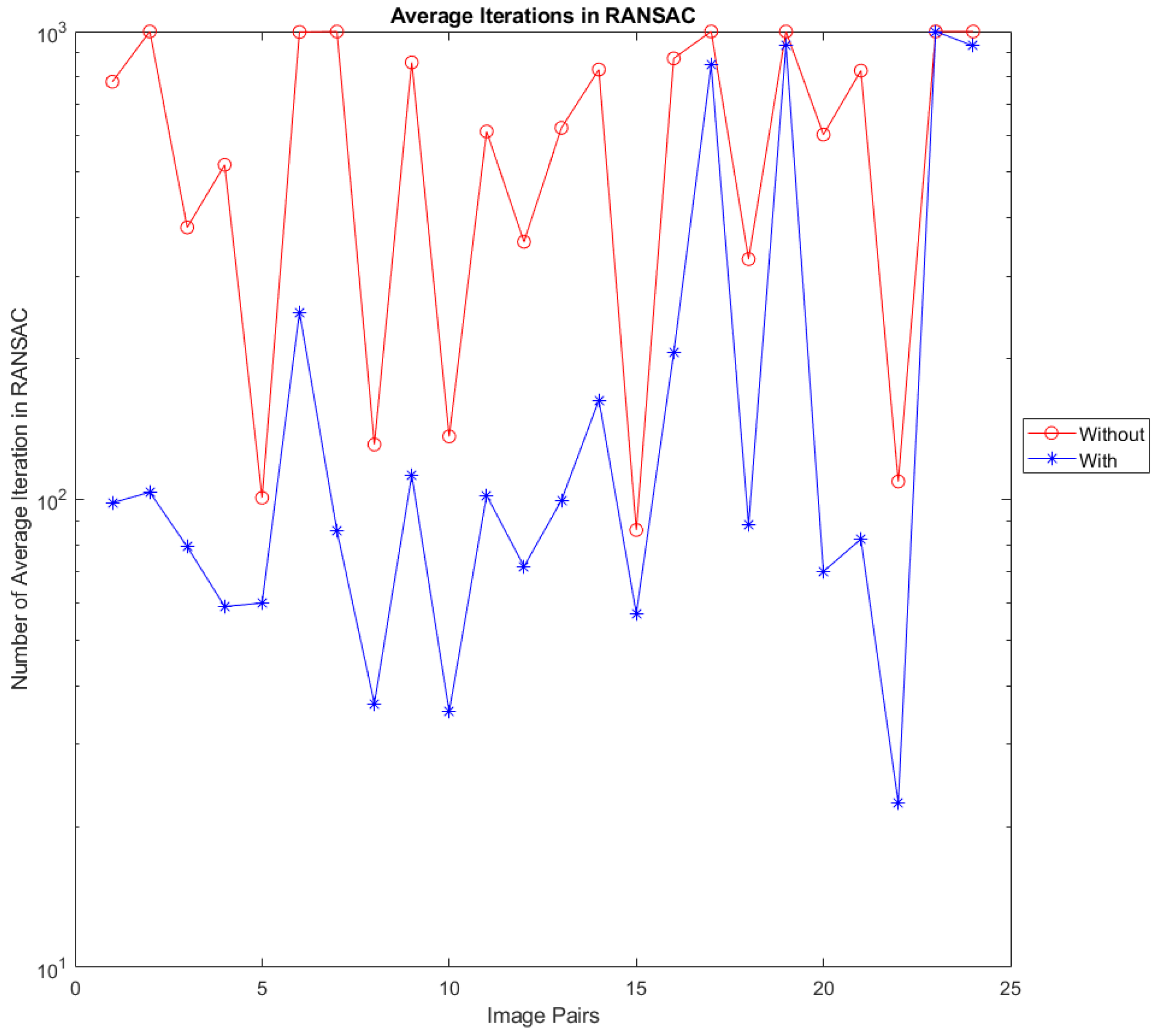
| Image Pair | Number of Corresp. | Number of Iterations in RANSAC | Number of Inliers | ||||||||||||||
|---|---|---|---|---|---|---|---|---|---|---|---|---|---|---|---|---|---|
| without | with | without | with | ||||||||||||||
| Min. | Max. | Avg. | Std. | Min. | Max. | Avg. | Std. | Min. | Max. | Avg. | Std. | Min. | Max. | Avg. | Std. | ||
| 1 | 236 | 514 | 1000 | 780.74 | 105.39 | 60 | 156 | 98.36 | 16.3 | 59 | 91 | 81.65 | 3.65 | 60 | 91 | 80.81 | 3.44 |
| 2 | 148 | 1000 | 1000 | 1000.00 | 0.00 | 89 | 208 | 103.60 | 15.3 | 6 | 19 | 16.78 | 2.92 | 17 | 19 | 18.33 | 0.70 |
| 3 | 354 | 234 | 635 | 381.24 | 63.43 | 52 | 124 | 79.21 | 12.8 | 109 | 148 | 134.34 | 4.68 | 80 | 146 | 131.45 | 6.98 |
| 4 | 526 | 356 | 732 | 518.77 | 68.83 | 40 | 94 | 59.04 | 9.08 | 110 | 140 | 130.93 | 5.35 | 77 | 124 | 107.60 | 7.22 |
| 5 | 680 | 68 | 152 | 100.81 | 14.14 | 41 | 87 | 60.05 | 8.25 | 255 | 315 | 300.17 | 9.9 | 258 | 314 | 300.06 | 9.08 |
| 6 | 252 | 881 | 1000 | 997.41 | 14.44 | 176 | 391 | 251.09 | 32 | 37 | 52 | 46.82 | 2.95 | 21 | 38 | 26.56 | 2.37 |
| 7 | 223 | 961 | 1000 | 999.84 | 2.46 | 50 | 166 | 85.69 | 17.8 | 32 | 50 | 48.66 | 2.82 | 45 | 51 | 49.32 | 0.60 |
| 8 | 375 | 84 | 230 | 131.02 | 24.90 | 24 | 70 | 36.61 | 7.78 | 171 | 194 | 184.26 | 2.7 | 167 | 191 | 184.84 | 1.62 |
| 9 | 268 | 583 | 1000 | 858.85 | 119.29 | 68 | 183 | 112.66 | 17.9 | 30 | 49 | 45.78 | 4.18 | 24 | 49 | 34.85 | 4.44 |
| 10 | 306 | 83 | 243 | 136.33 | 26.13 | 18 | 65 | 35.20 | 7.62 | 155 | 164 | 159.09 | 1.99 | 156 | 163 | 159.78 | 0.80 |
| 11 | 249 | 385 | 903 | 611.46 | 85.97 | 71 | 158 | 101.98 | 15 | 55 | 84 | 77.00 | 2.54 | 70 | 82 | 76.28 | 2.46 |
| 12 | 293 | 261 | 554 | 355.28 | 49.98 | 48 | 114 | 71.88 | 11.4 | 94 | 111 | 102.77 | 2.45 | 69 | 105 | 95.56 | 5.21 |
| 13 | 304 | 406 | 942 | 622.35 | 80.30 | 57 | 152 | 99.56 | 16.6 | 39 | 65 | 54.69 | 3.91 | 39 | 66 | 56.15 | 4.38 |
| 14 | 360 | 582 | 1000 | 829.27 | 92.79 | 114 | 223 | 163.05 | 21.7 | 79 | 106 | 92.63 | 3.77 | 80 | 106 | 91.42 | 3.27 |
| 15 | 839 | 53 | 128 | 86.03 | 13.04 | 36 | 91 | 57.06 | 9.34 | 327 | 417 | 390.33 | 15.3 | 320 | 416 | 390.99 | 15.47 |
| 16 | 266 | 570 | 1000 | 876.05 | 102.93 | 162 | 367 | 205.72 | 35.5 | 54 | 77 | 66.06 | 3.07 | 22 | 61 | 43.79 | 9.97 |
| 17 | 166 | 1000 | 1000 | 1000.00 | 0.00 | 699 | 1000 | 847.74 | 97.9 | 18 | 31 | 25.24 | 2.9 | 14 | 24 | 21.89 | 1.73 |
| 18 | 406 | 198 | 554 | 326.17 | 57.14 | 47 | 151 | 88.10 | 15.7 | 139 | 179 | 167.56 | 6.96 | 127 | 180 | 166.12 | 7.99 |
| 19 | 138 | 1000 | 1000 | 1000.00 | 0.00 | 680 | 1000 | 933.63 | 125 | 5 | 16 | 13.10 | 2.09 | 5 | 16 | 13.30 | 1.95 |
| 20 | 200 | 414 | 913 | 601.97 | 71.21 | 44 | 111 | 70.13 | 9.96 | 55 | 67 | 58.14 | 2.76 | 55 | 66 | 58.16 | 2.00 |
| 21 | 196 | 531 | 1000 | 824.81 | 118.15 | 46 | 130 | 82.28 | 14.9 | 26 | 40 | 36.37 | 2.72 | 19 | 36 | 29.98 | 2.08 |
| 22 | 290 | 69 | 194 | 109.24 | 18.91 | 13 | 44 | 22.47 | 4.35 | 90 | 116 | 109.81 | 4.34 | 95 | 116 | 109.37 | 4.17 |
| 23 | 171 | 1000 | 1000 | 1000.00 | 0.00 | 1000 | 1000 | 1000.00 | 0 | 13 | 32 | 24.75 | 3.43 | 13 | 31 | 25.70 | 4.08 |
| 24 | 148 | 1000 | 1000 | 1000.00 | 0.00 | 737 | 1000 | 931.62 | 112 | 4 | 16 | 11.80 | 2.12 | 10 | 14 | 11.39 | 1.56 |
| Image Pair | Number of Corresp. | Number of Iterations in RANSAC | Number of Inliers | ||||||||||||||
|---|---|---|---|---|---|---|---|---|---|---|---|---|---|---|---|---|---|
| without | with | without | with | ||||||||||||||
| Min. | Max. | Avg. | Std. | Min. | Max. | Avg. | Std. | Min. | Max. | Avg. | Std. | Min. | Max. | Avg. | Std. | ||
| 2 | 533 | 1000 | 1000 | 1000 | 0 | 21 | 57 | 29.00 | 4.88 | 47 | 93 | 88.62 | 3.31 | 84 | 91 | 88.807 | 1.04 |
| 17 | 545 | 1000 | 1000 | 1000 | 0 | 59 | 214 | 122.04 | 22.70 | 5 | 60 | 38.23 | 10.53 | 35 | 57 | 49.284 | 4.94 |
| 19 | 406 | 1000 | 1000 | 1000 | 0 | 459 | 1000 | 680.11 | 135.27 | 4 | 23 | 10.37 | 5.25 | 14 | 24 | 21.879 | 0.65 |
| 21 | 500 | 1000 | 1000 | 1000 | 0 | 86 | 292 | 160.86 | 36.00 | 30 | 57 | 50.80 | 6.43 | 24 | 35 | 31.176 | 2.23 |
| 23 | 457 | 1000 | 1000 | 1000 | 0 | 356 | 916 | 650.29 | 94.78 | 8 | 49 | 36.64 | 7.34 | 21 | 48 | 42.496 | 3.62 |
| 24 | 439 | 1000 | 1000 | 1000 | 0 | 1000 | 1000 | 1000.00 | 0.00 | 4 | 25 | 15.24 | 5.46 | 0 | 4 | 2.336 | 1.97 |
© 2019 by the authors. Licensee MDPI, Basel, Switzerland. This article is an open access article distributed under the terms and conditions of the Creative Commons Attribution (CC BY) license (http://creativecommons.org/licenses/by/4.0/).
Share and Cite
Elibol, A.; Chong, N.Y. Efficient Image Registration for Underwater Optical Mapping Using Geometric Invariants. J. Mar. Sci. Eng. 2019, 7, 178. https://doi.org/10.3390/jmse7060178
Elibol A, Chong NY. Efficient Image Registration for Underwater Optical Mapping Using Geometric Invariants. Journal of Marine Science and Engineering. 2019; 7(6):178. https://doi.org/10.3390/jmse7060178
Chicago/Turabian StyleElibol, Armagan, and Nak Young Chong. 2019. "Efficient Image Registration for Underwater Optical Mapping Using Geometric Invariants" Journal of Marine Science and Engineering 7, no. 6: 178. https://doi.org/10.3390/jmse7060178
APA StyleElibol, A., & Chong, N. Y. (2019). Efficient Image Registration for Underwater Optical Mapping Using Geometric Invariants. Journal of Marine Science and Engineering, 7(6), 178. https://doi.org/10.3390/jmse7060178