Kelvin-Helmholtz Billows Induced by Shear Instability along the North Passage of the Yangtze River Estuary, China


Abstract
1. Introduction
2. Methodology
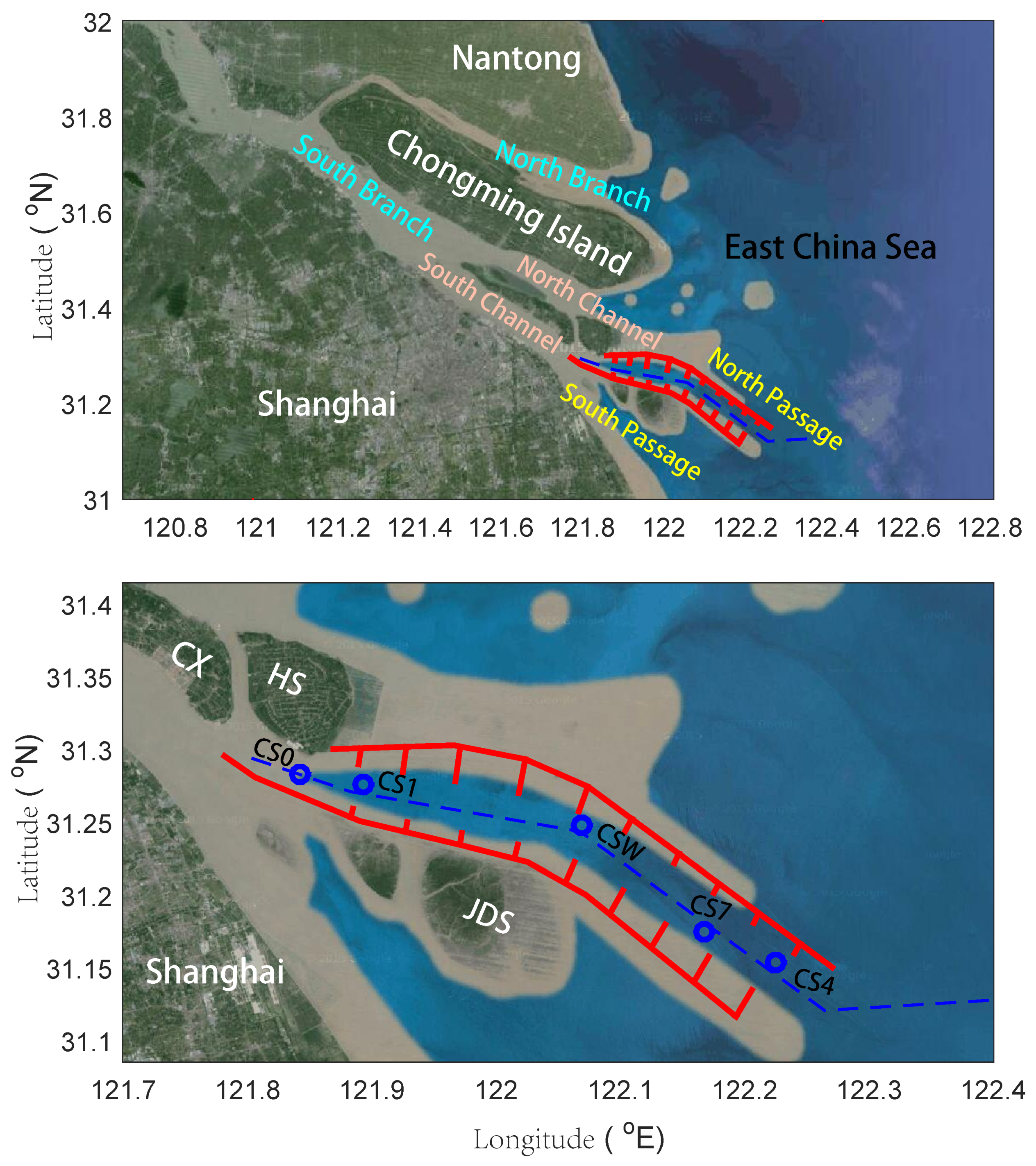
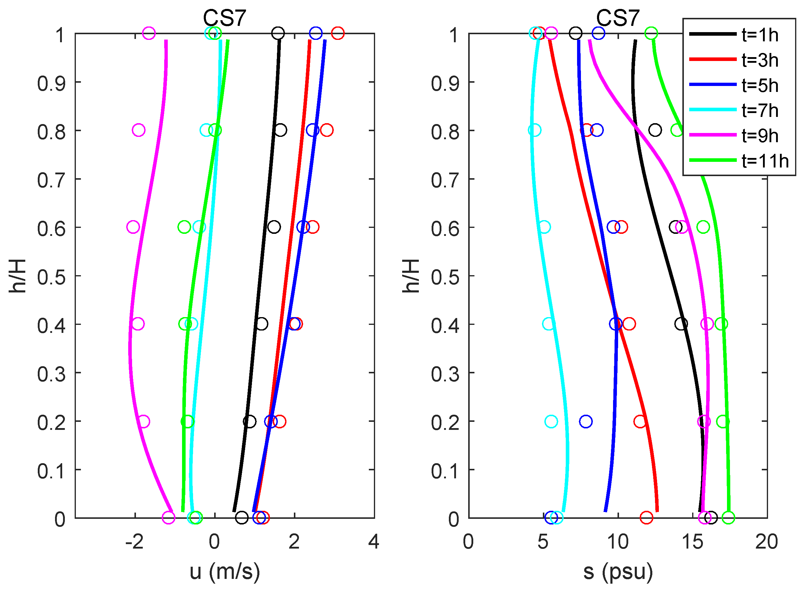
2.1. Study Area
2.2. Numerical Model
2.2.1. Governing Equations
2.2.2. Numerical Approach
2.3. Model Setup
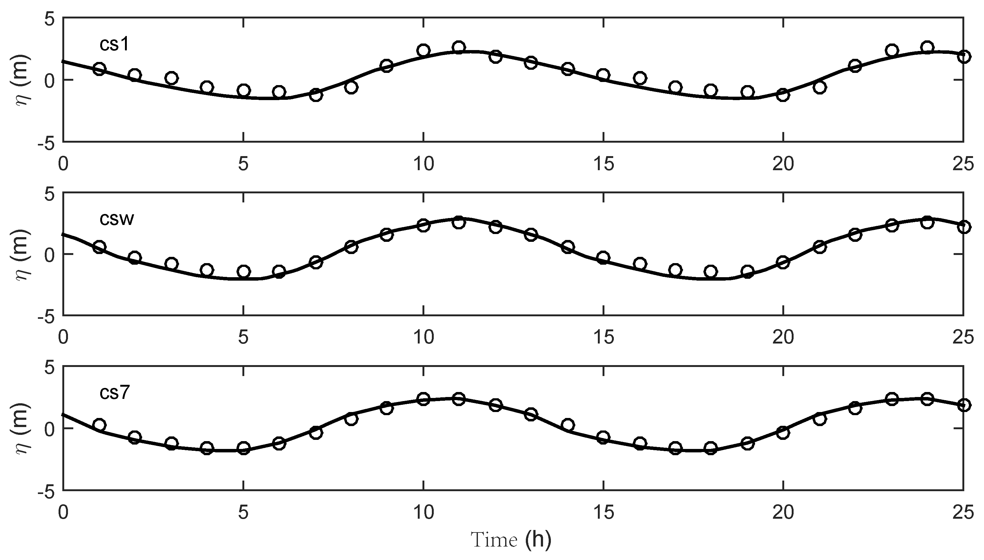
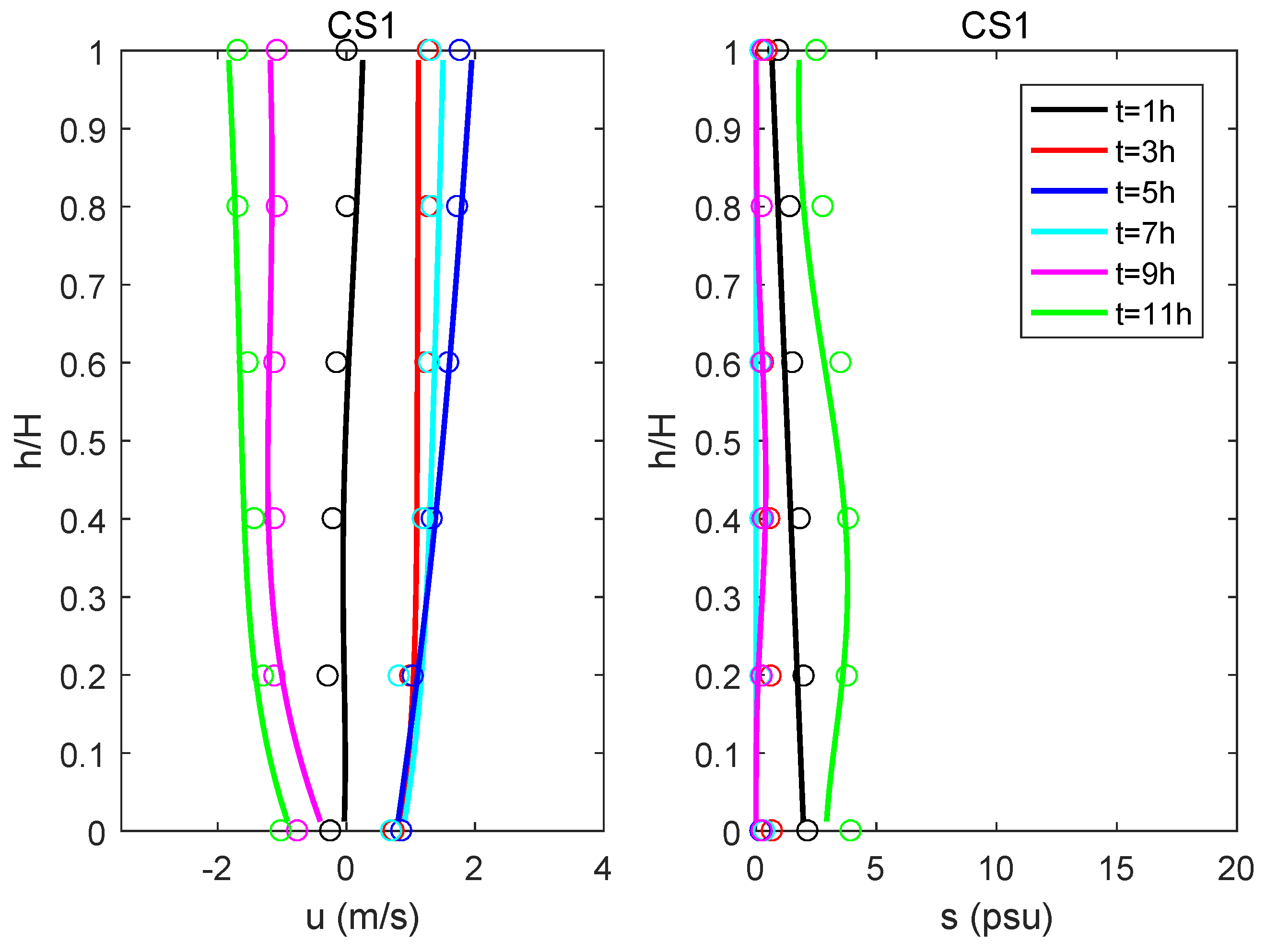
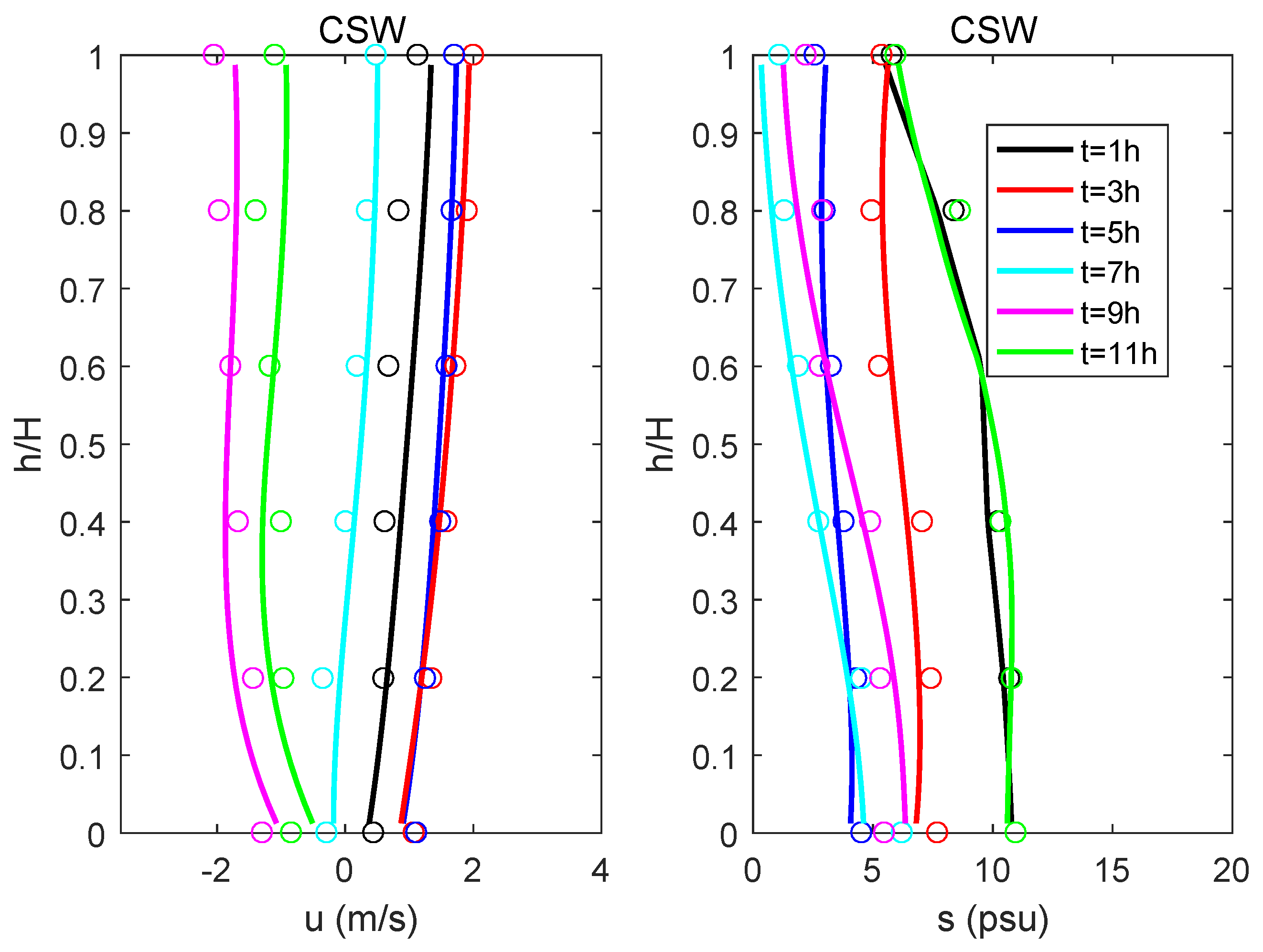
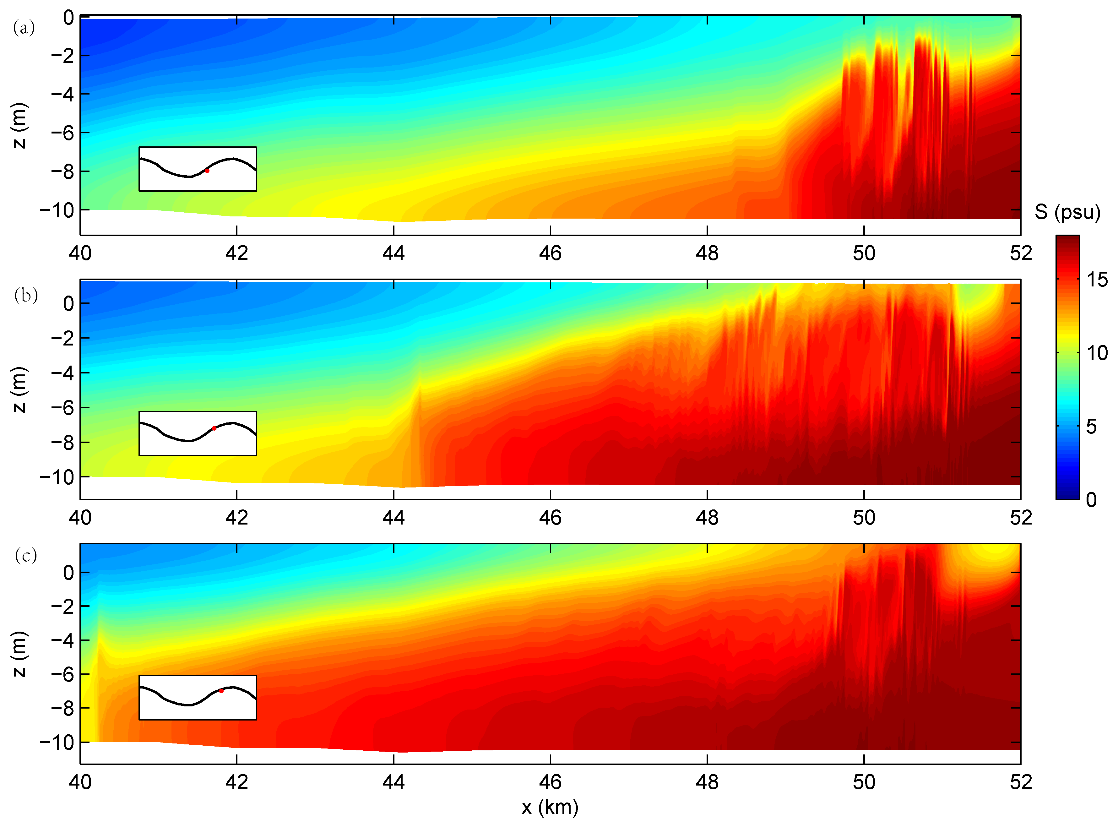
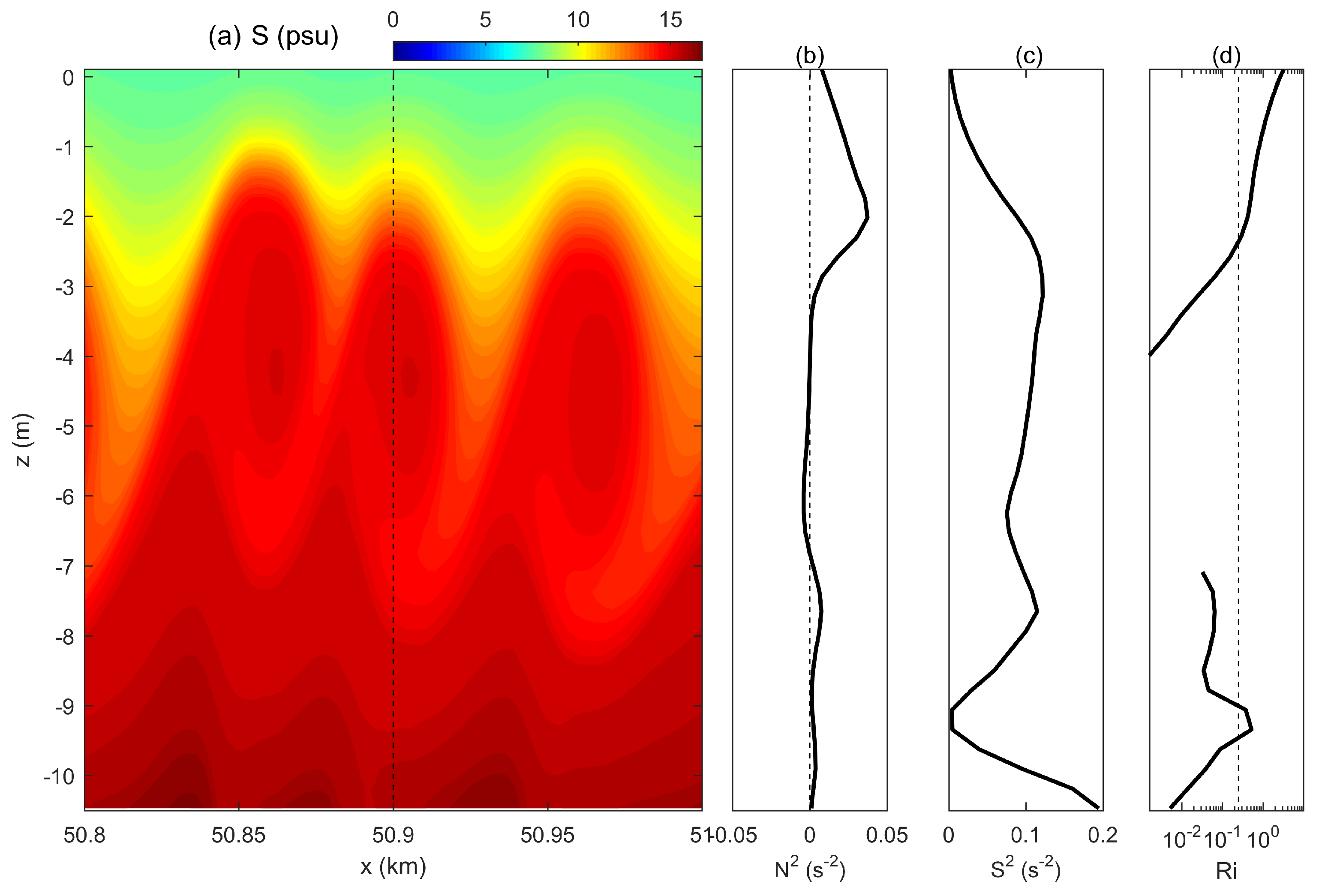
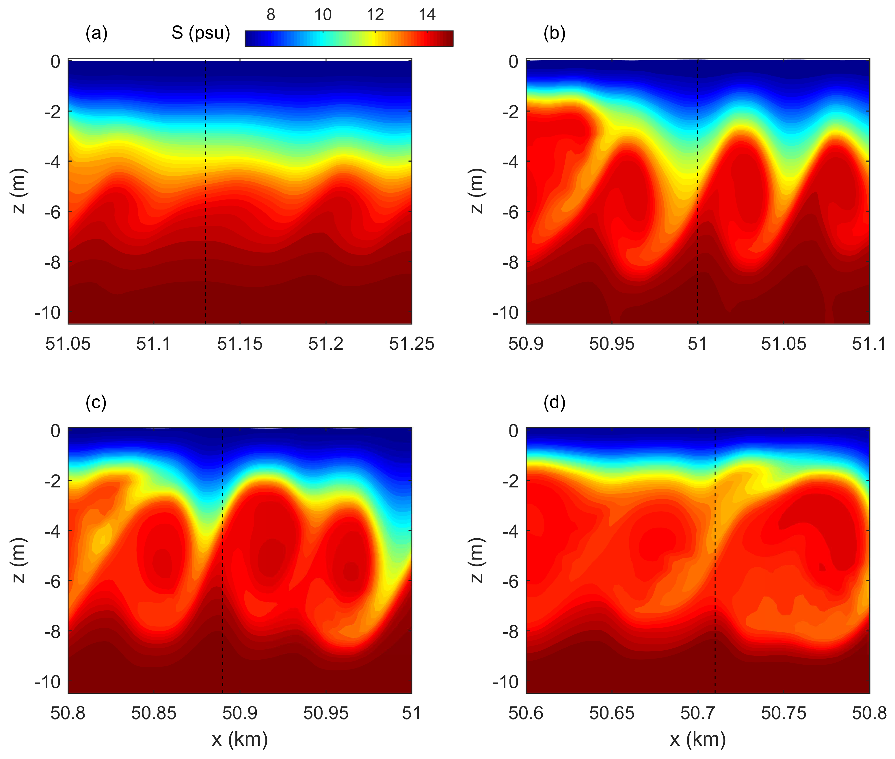
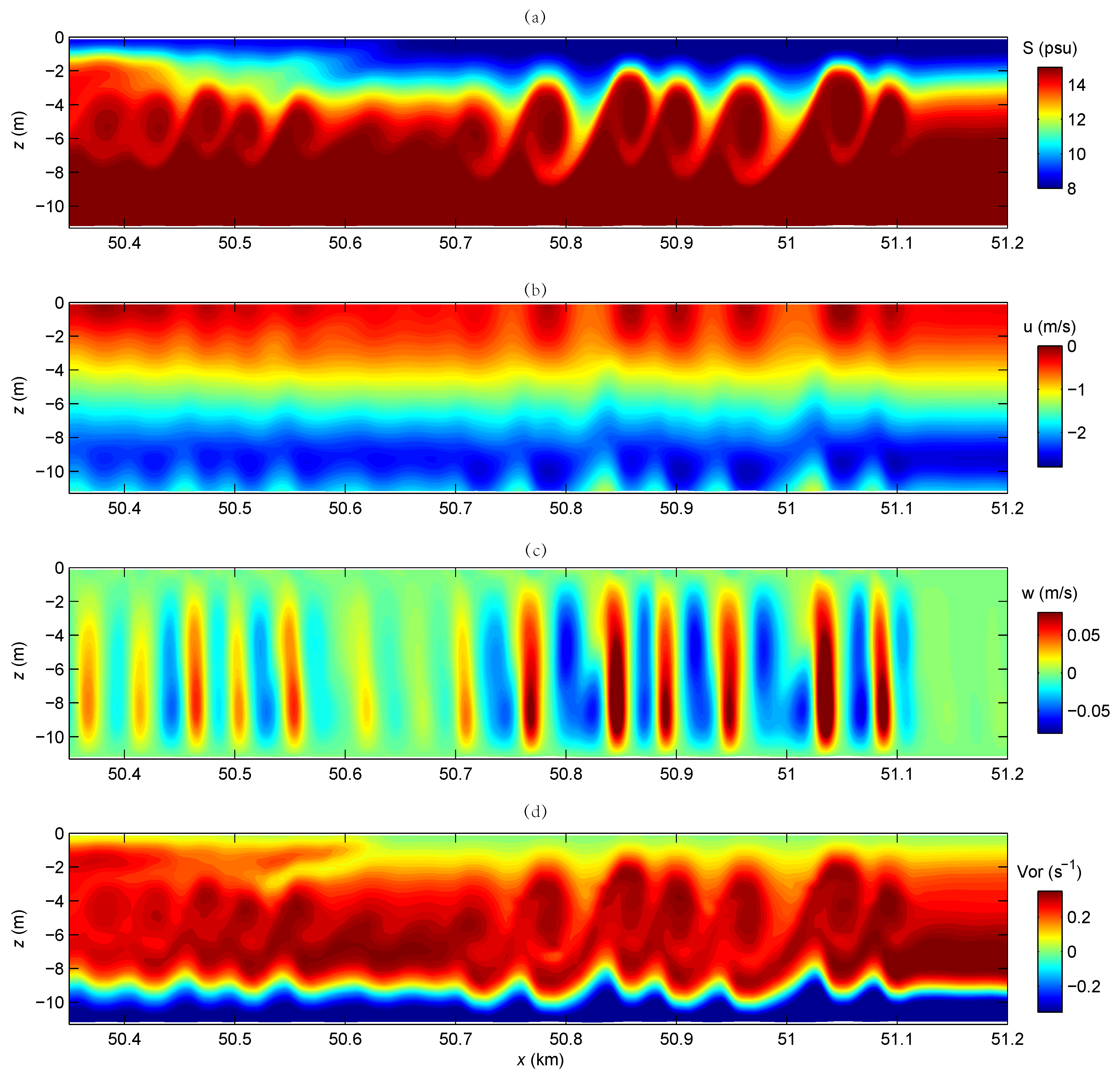
3. Model Results
4. Discussion
4.1. The Existence of K-H Instability
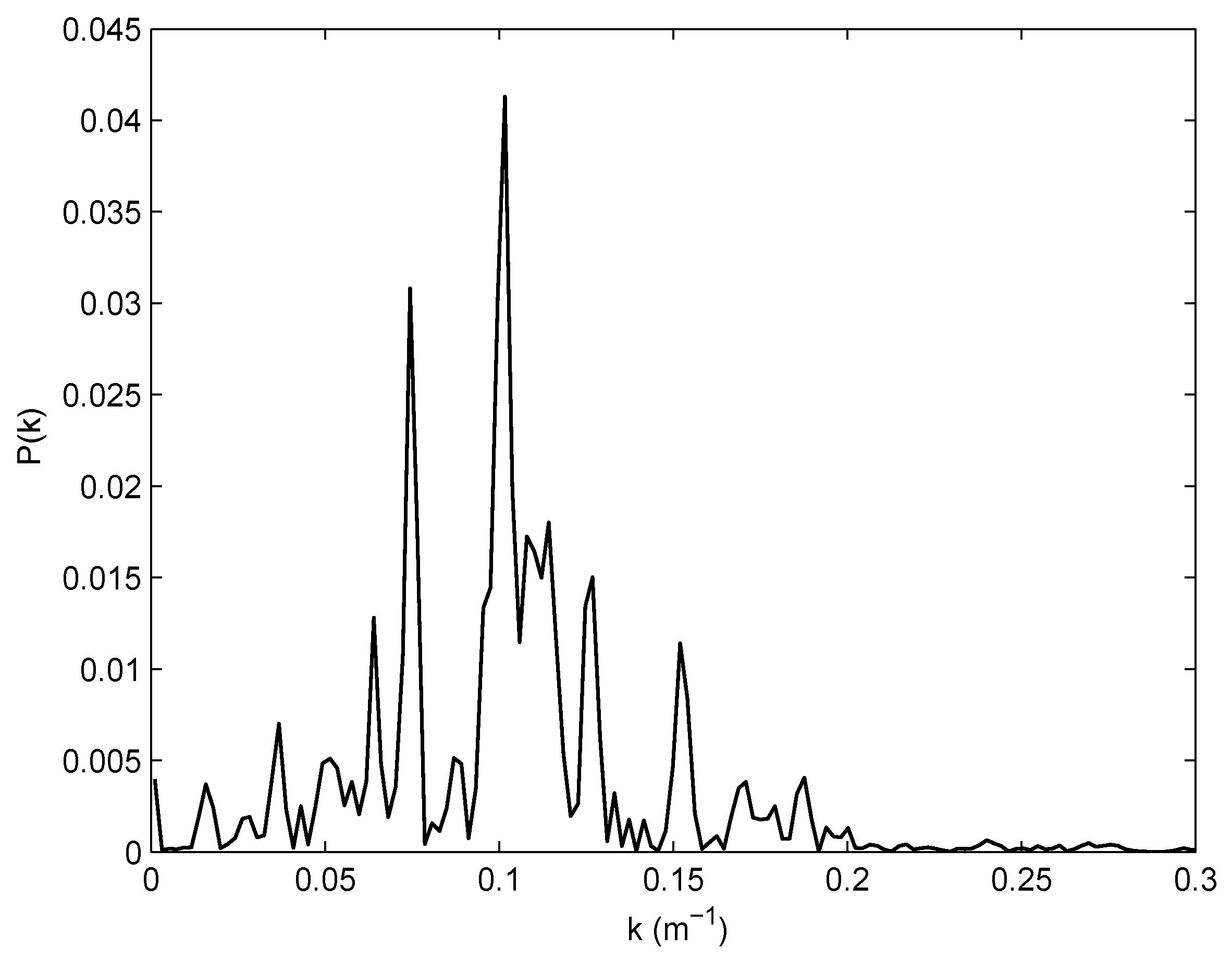
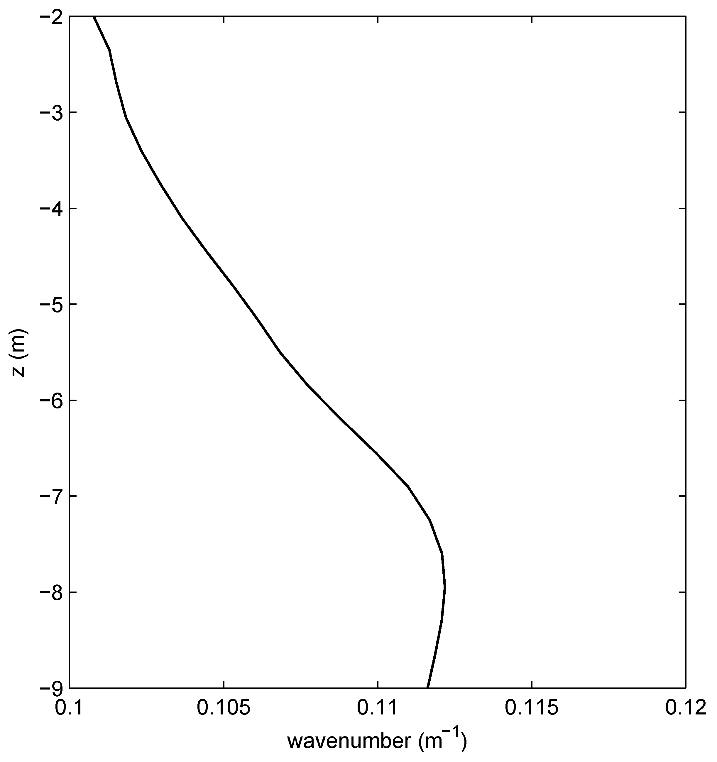
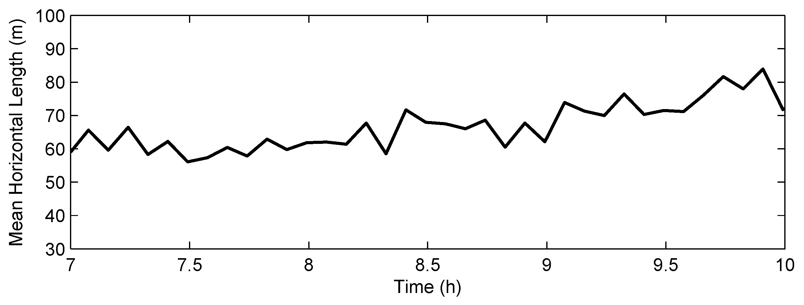
4.2. The Spatial and Temporal Scales of the K-H Billows
4.3. Mixing Efficiency
5. Conclusions
Author Contributions
Funding
Acknowledgments
Conflicts of Interest
References
- Hu, K.; Ding, P.; Wang, Z.; Yang, S. A 2D/3D hydrodynamic and sediment transport model for the Yangtze Estuary, China. J. Mar. Syst. 2009, 77, 114–136. [Google Scholar] [CrossRef]
- Zheng, J.; Zhang, C.; Demirbilek, Z.; Lin, L. Numerical study of sandbar migration under wave-undertow interaction. J. Waterw. Port Coast. Ocean Eng. 2014, 140, 146–159. [Google Scholar] [CrossRef]
- Zhang, C.; Zhang, Q.; Zheng, J.; Demirbilek, Z. Parameterization of nearshore wave front slope. Coast. Eng. 2017, 127, 80–87. [Google Scholar] [CrossRef]
- Horner-Devine, A.R.; Hetland, R.D.; MacDonald, D.G. Mixing and transport in coastal river plumes. Annu. Rev. Fluid Mech. 2015, 47, 569–594. [Google Scholar] [CrossRef]
- Shi, J.; Zheng, J.; Tong, C. Non-hydrostatic modelling if Kelvin-Helmholtz billows along the North Passage of Yangtze River Estuary, China. Coast. Eng. Proc. 2018, 1, 81. [Google Scholar] [CrossRef]
- Chen, W.Y.; Chen, G.X.; Chen, W.; Liao, C.C.; Gao, H.M. Numerical simulation of the nonlinear wave-induced dynamic response of anisotropic poro-elastoplastic seabed. Mar. Georesour. Geotechnol. 2018, 1–12. [Google Scholar] [CrossRef]
- Liao, C.; Tong, D.; Jeng, D.S.; Zhao, H. Numerical study for wave-induced oscillatory pore pressures and liquefaction around impermeable slope breakwater heads. Ocean Eng. 2018, 157, 364–375. [Google Scholar] [CrossRef]
- Thomson, W. Hydrokinetic solutions and observations. Philos. Mag. 1871, 42, 362–377. [Google Scholar] [CrossRef]
- Von Helmholtz, H. Die energie der wogen und des windes. Ann. Phys. 1890, 277, 641–662. [Google Scholar] [CrossRef]
- Miles, J.W. On the stability of heterogeneous shear flows. J. Fluid Mech. 1961, 10, 496–508. [Google Scholar] [CrossRef]
- Howard, L.N. Note on a paper of John W. Miles. J. Fluid Mech. 1961, 10, 509–512. [Google Scholar] [CrossRef]
- Hazel, P. Numerical studies of the stability of inviscid parallel shear flows. J. Fluid Mech. 1972, 39, 39–61. [Google Scholar]
- Fringer, O.B.; Street, R.L. The dynamics of breaking progressive interfacial waves. J. Fluid Mech. 2003, 494, 319–353. [Google Scholar] [CrossRef]
- Barad, M.F.; Fringer, O.B. Simulations of shear instabilities in interfacial gravity waves. J. Fluid Mech. 2010, 644, 61–95. [Google Scholar] [CrossRef]
- Fructus, D.; Carr, M.; Grue, J.; Jensen, A.; Davies, P.A. Shear-induced breaking of large internal solitary waves. J. Fluid Mech. 2009, 620, 1–29. [Google Scholar] [CrossRef]
- Troy, C.D.; Koseff, J.R. The instability and breaking of long internal waves. J. Fluid Mech. 2005, 543, 107–136. [Google Scholar] [CrossRef]
- Woods, J.D. Wave-induced shear instability in the summer thermocline. J. Fluid Mech. 1968, 32, 791–800. [Google Scholar] [CrossRef]
- Geyer, W.R.; Smith, J.D. Shear instability in a highly stratified estuary. J. Phys. Oceanogr. 1987, 17, 1668–1679. [Google Scholar] [CrossRef]
- Geyer, W.R.; Farmer, D.M. Tide-induced variation of the dynamics of a salt wedge estuary. J. Phys. Oceanogr. 1989, 19, 1060–1072. [Google Scholar] [CrossRef]
- Bourgault, D.; Saucier, F.J.; Lin, C.A. Shear instability in the St. Lawrence Estuary, Canada: A comparison of fine-scale observations and estuarine circulation model results. J. Geophys. Res. Oceans 2001, 106, 9393–9409. [Google Scholar] [CrossRef]
- Geyer, W.R.; Lavery, A.C.; Scully, M.E.; Trowbridge, J.H. Mixing by shear instability at high Reynolds number. Geophys. Res. Lett. 2010, 37, L22607. [Google Scholar] [CrossRef]
- Tedford, E.W.; Carpenter, J.R.; Pawlowicz, R.; Pieters, R.; Lawrence, G.A. Observation and analysis of shear instability in the Fraser River estuary. J. Geophys. Res. Oceans 2009, 114, C11006. [Google Scholar] [CrossRef]
- Chang, M.H.; Jheng, S.Y.; Lien, R.C. Trains of large Kelvin-Helmholtz billows observed in the Kuroshio above a seamount. Geophys. Res. Lett. 2016, 43, 8654–8661. [Google Scholar] [CrossRef]
- Marmorino, G.O. Observations of small-scale mixing processes in the seasonal thermocline, Part II: Wave breaking. J. Phys. Oceanogr. 1987, 17, 1348–1355. [Google Scholar] [CrossRef]
- Lavery, A.C.; Chu, D.; Moum, J.N. Measurements of acoustic scattering from zooplankton and oceanic microstructure using a broadband echosounder. J. Mar. Sci. 2009, 67, 379–394. [Google Scholar] [CrossRef]
- Shchepetkin, A.F.; McWilliams, J.C. The regional oceanic modeling system (ROMS): A split-explicit, free-surface, topography-following-coordinate oceanic model. Ocean Model. 2005, 9, 347–404. [Google Scholar] [CrossRef]
- Chen, X. A fully hydrodynamic model for three-dimensional, free-surface flows. Int. J. Numer. Methods Fluids 2003, 42, 929–952. [Google Scholar] [CrossRef]
- Stelling, G.W. On the Construction of Computational Methods for Shallow Water Flow Problems; Technical Report 35; Rijkwaterstaat: Dutch, The Netherlands, 1984.
- Stelling, G.W. Practical aspects of accurate tidal computations. J. Hydraul. Eng. 1986, 112, 802–817. [Google Scholar] [CrossRef]
- Özgökmen, T.M.; Johns, W.E.; Peters, H.; Matt, S. Turbulent mixing in the Red Sea outflow plume from a high-resolution nonhydrostatic model. J. Phys. Oceanogr. 2003, 33, 1846–1869. [Google Scholar] [CrossRef]
- Wang, B.; Fringer, O.B.; Giddings, S.N.; Fong, D.A. High-resolution simulations of a macrotidal estuary using SUNTANS. Ocean Model. 2009, 28, 167–192. [Google Scholar] [CrossRef]
- Fringer, O.; Gerritsen, M.; Street, R. An unstructured-grid, finite-volume, nonhydrostatic, parallel coastal ocean simulator. Ocean Model. 2006, 14, 139–173. [Google Scholar] [CrossRef]
- Vlasenko, V.; Stashchuk, N.; McEwan, R. High-resolution modelling of a large-scale river plume. Ocean Dyn. 2013, 63, 1307–1320. [Google Scholar] [CrossRef]
- Lu, S.; Tong, C.; Lee, D.Y.; Zheng, J.; Shen, J.; Zhang, W.; Yan, Y. Propagation of tidal waves up in Yangtze Estuary during the dry season. J. Geophys. Res. Oceans 2015, 120, 6445–6473. [Google Scholar] [CrossRef]
- Shi, Z.; Li, C.; Dou, X. Three-dimensional modeling of tidal circulation within the north and south passages of the partially-mixed Changjiang River Estuary, China. J. Hydrodyn. 2010, 22, 656–661. [Google Scholar] [CrossRef]
- Li, L.; Zhu, J.; Wu, H. Impacts of wind stress on saltwater intrusion in the Yangtze Estuary. Sci. China Earth Sci. 2012, 55, 1178–1192. [Google Scholar] [CrossRef]
- Li, L.; He, Z.; Xia, Y.; Dou, X. Dynamics of sediment transport and stratification in Changjiang River Estuary, China. Estuarine. Coast. Shelf Sci. 2018, 213, 1–17. [Google Scholar] [CrossRef]
- Zhang, M.; Townend, I.; Cai, H.; He, J.; Mei, X. The influence of seasonal climate on the morphology of the mouth-bar in the Yangtze Estuary, China. Cont. Shelf Res. 2018, 153, 30–49. [Google Scholar] [CrossRef]
- Pu, X.; Shi, J.Z.; Hu, G.D.; Xiong, L.B. Circulation and mixing along the North Passage in the Changjiang River estuary, China. J. Mar. Syst. 2015, 148, 213–235. [Google Scholar] [CrossRef]
- Ma, G.; Shi, F.; Kirby, J.T. Shock-capturing non-hydrostatic model for fully dispersive surface wave processes. Ocean Model. 2012, 43–44, 22–35. [Google Scholar] [CrossRef]
- Ma, G.; Kirby, J.T.; Shi, F. Numerical simulation of tsunami waves generated by deformable submarine landslides. Ocean Model. 2013, 69, 146–165. [Google Scholar] [CrossRef]
- Shi, J.; Shi, F.; Kirby, J.T.; Ma, G.; Wu, G.; Tong, C.; Zheng, J. Pressure Decimation and Interpolation (PDI) method for a baroclinic non-hydrostatic model. Ocean Model. 2015, 96, 265–279. [Google Scholar] [CrossRef]
- Shi, F.; Kirby, J.T.; Harris, J.C.; Geiman, J.D.; Grilli, S.T. A high-order adaptive time-stepping TVD solver for Boussinesq modeling of breaking waves and coastal inundation. Ocean Model. 2012, 43, 36–51. [Google Scholar] [CrossRef]
- Liang, Q.; Marche, F. Numerical resolution of well-balanced shallow water equations with complex source terms. Adv. Water Resour. 2009, 32, 873–884. [Google Scholar] [CrossRef]
- Stelling, G.; Zijlema, M. An accurate and efficient finite-difference algorithm for non-hydrostatic free-surface flow with application to wave propagation. Int. J. Numer. Methods Fluids 2003, 43, 1–23. [Google Scholar] [CrossRef]
- Harten, A.; Lax, P.; van Leer, B. On upstream differencing and Godunov-type schemes for hyperbolic conservation laws. SIAM Rev. 1983, 25, 35–61. [Google Scholar] [CrossRef]
- Toro, E.F.; Spruce, M.; Speares, W. Restoration of the contact surface in the HLL-Riemann solver. Shock Waves 1994, 4, 25–34. [Google Scholar] [CrossRef]
- Pacanowski, R.C.; Philander, S.G.H. Parameterization of vertical mixing in numerical models of tropical oceans. J. Phys. Oceanogr. 1981, 11, 1443–1451. [Google Scholar] [CrossRef]
- Large, W.G.; McWilliams, J.C.; Doney, S.C. Oceanic vertical mixing: A review and a model with a nonlocal boundary layer parameterization. Rev. Geophys. 1994, 32, 363–403. [Google Scholar] [CrossRef]
- Corcos, G.M.; Sherman, F.S. Vorticity concentration and the dynamics of unstable free shear layers. J. Fluid Mech. 1976, 73, 241–264. [Google Scholar] [CrossRef]
- Winters, K.B.; Lombard, P.N.; Riley, J.J.; D’Asaro, E.A. Available potential energy and mixing in density-stratified fluids. J. Fluid Mech. 1995, 289, 115–128. [Google Scholar] [CrossRef]
- Dossmann, Y.; Rosevear, M.G.; Griffiths, R.W.; McC. Hogg, A.; Hughes, G.O.; Copeland, M. Experiments with mixing in stratified flow over a topographic ridge. J. Geophys. Res. Oceans 2016, 121, 6961–6977. [Google Scholar] [CrossRef]


© 2019 by the authors. Licensee MDPI, Basel, Switzerland. This article is an open access article distributed under the terms and conditions of the Creative Commons Attribution (CC BY) license (http://creativecommons.org/licenses/by/4.0/).
Share and Cite
Shi, J.; Tong, C.; Zheng, J.; Zhang, C.; Gao, X. Kelvin-Helmholtz Billows Induced by Shear Instability along the North Passage of the Yangtze River Estuary, China. J. Mar. Sci. Eng. 2019, 7, 92. https://doi.org/10.3390/jmse7040092
Shi J, Tong C, Zheng J, Zhang C, Gao X. Kelvin-Helmholtz Billows Induced by Shear Instability along the North Passage of the Yangtze River Estuary, China. Journal of Marine Science and Engineering. 2019; 7(4):92. https://doi.org/10.3390/jmse7040092
Chicago/Turabian StyleShi, Jian, Chaofeng Tong, Jinhai Zheng, Chi Zhang, and Xiangyu Gao. 2019. "Kelvin-Helmholtz Billows Induced by Shear Instability along the North Passage of the Yangtze River Estuary, China" Journal of Marine Science and Engineering 7, no. 4: 92. https://doi.org/10.3390/jmse7040092
APA StyleShi, J., Tong, C., Zheng, J., Zhang, C., & Gao, X. (2019). Kelvin-Helmholtz Billows Induced by Shear Instability along the North Passage of the Yangtze River Estuary, China. Journal of Marine Science and Engineering, 7(4), 92. https://doi.org/10.3390/jmse7040092