Article

Ship Manoeuvrability-Based Simulation for Ship Navigation in Collision Situations

Navigation College, Dalian Maritime University, Dalian 116026, China
*
Author to whom correspondence should be addressed.
J. Mar. Sci. Eng. 2019, 7(4), 90; https://doi.org/10.3390/jmse7040090
Submission received: 28 February 2019 / Revised: 25 March 2019 / Accepted: 26 March 2019 / Published: 30 March 2019

Abstract

:
In this article, a ship manoeuvrability-based simulation for ship navigation in collision situations is established. Under the general requirement from the Convention on the International Regulations for Preventing Collisions at Sea (COLREGs) and good seamanship, the determination of encounter situations is quantified to reduce navigators’ intervention. Meanwhile, the action manner by course alteration or changing speed in some typical encounter situations is graphically analysed for both the give-way and stand-on vessels. Then, the multiple genetic algorithm and linear extension algorithm are adopted to perform trajectory planning for collision avoidance. To improve the reliability of the simulation system, the mathematical model of ship motion and ship manoeuvring control mechanism are adopted, which can eliminate the insufficiency of neglect of ship manoeuvrability in the process of collision avoidance. Meanwhile, the course encoding technique is adopted to fit the ship manoeuvring control mechanism. Finally, a set of traffic scenarios emulating different encounter situations are applied to demonstrate the effectiveness, consistency, and practicality of this system.

1. Introduction

With the recent growing interest in the ocean for civilian and military applications, there has been increasing demand for the autonomy of unmanned surface vehicles (USVs). For example, in 2005, e-navigation was an initiative started by the International Maritime Origination (IMO) to increase navigation safety by using modern technology. In 2012, the European Union invested in the Maritime Unmanned Navigation through Intelligence in Networks (MUNIN) project to develop an autonomous dry bulk carrier. In 2015, the Finnish Funding Agency approved the academic research project—Advanced Autonomous Waterborne Applications (AAWA). In 2016, Rolls-Royce published their plan for the construction of autonomous ships. In 2018, the IMO published the degree level on Maritime Autonomous Surface Ship (MASS). Through years of progress, many decision support systems have achieved significant results [1,2,3,4,5,6,7,8,9,10]. For example, Szlapczynski [6] presented the evolutionary sets of safe trajectories (ESoSST) to obtain a set of trajectories of all the ships instead of just one ship; Tam [7] determined priority based on the Convention on the International Regulations for Preventing Collisions at Sea (COLREGs) [11] and ship manoeuvrability, standardized the evasive turning angle for all vessels to 30°, and then determined the linear extension after the evasive manoeuvre; Tsou [8] integrated a geographic information system (GIS) module to conduct obstacle avoidance processing and selection of a route; Sun [12] established a collision avoidance system based on finite control set model predictive control (FCS-MPC); and Lv [13] adopted a modified Artificial Potential Field (APF) to realize real-time and deterministic path planning. Among these results, the simulation for ship navigation could be a powerful tool for operational planning and design studies of waterways [14]. The key technology is to determine the encounter situation and perform autonomous trajectory finding in collision situations with no or minimum intervention of navigators.
Nevertheless, the above-mentioned decision support systems lay emphasis on trajectory optimization, thus the encounter situation is usually a prior assumption in the simulation based on Rules 13–15 of COLREGs. In fact, the determination of an encounter situation, which classifies the avoidance responsibility and confirms the action time horizon, is an important precondition for trajectory optimization. To improve the autonomy of this simulation system, the qualitative provisions are materialized with the quantified criteria including collision risk verification, crossing angle bearing orientation, and applicable distance. The concept of risk of collision interpreted in Rule 7 is an important condition. In practice, the distance of the closest point of approach (DCPA) and the time of the closest point of approach (TCPA) for the two approaching vessels are the most important factors in determining whether the risk of collision exists [15]. Considering the visible range of lights defined in Rule 22 and navigational practice, the applicable distance at which an encounter situation applies is analysed. More importantly, to ensure evasive action compliance with navigational practice and reduce the doubt about the evasive manoeuvre especially in encounters between ships with this automatic simulation system and ships without this system, the action manners, including course alteration and changing speed for different encounter situations, are analysed based on COLREGs, good seamanship, and the cost of avoidance.
The optimization methods for trajectory planning have been previously reviewed and discussed [16]. In general, the methods can be divided into two groups, the deterministic approach and the heuristic approach. The former calculates and determines the final decision in strict accordance with the defined process characterized by a low dimensional state space (typically up to two dimensions); the latter is to search inside a subspace of the search space for an acceptable solution rather than the best solution that satisfies the design requirement. Nevertheless, each approach has its limitations. For the deterministic approach, it is constrained by the optimization ability to only deal with a single variable. Therefore, it usually applies a distributed computing method to calculate the optimal trajectory with a prior assumption of other relevant parameters. Moreover, the obtained optimal trajectory just returned to the original course rather than the original track, whereas, in practice, the give-way ship should return to the original track as much as possible once the risk of collision is cleared. For the heuristic approach, trajectory planning is required to generate a sequence of actions from a start position to the original track. Considering the presence of random variables in large quantities in the process of optimization, the evasive manoeuvre usually covers many times of course alteration, so the consistency of the optimal solution cannot be guaranteed, which is not compliant with navigational practice. In addition, with the heuristic approach it is easy to trap in the trouble of premature convergence.
It is remarkable that there is one common shortage in the above-mentioned research, most of the published methods are characterized by an idealised mathematical model of ship motion without considering ship manoeuvrability in the process of trajectory planning. Generally speaking, ship manoeuvrability weighs the response capability when a ship is handled by an operator or interfered with by an external environment [17]. Therefore, ship manoeuvrability is a major and important issue for the simulation of ship navigation, especially in collision situations when a series of actions are taken.
Motivated by the mentioned observations, a ship manoeuvrability-based simulation for ship navigation in collision situations is presented in this paper. Under the general requirements of COLREGs and good seamanship, the determination of an encounter situation is quantified to reduce the intervention of navigators. Meanwhile, the action manner by course alteration or changing speed in some typical encounter situations is graphically analysed for both give-way and stand-on vessels. For the manner of course alteration, the authors have recently reported a trajectory planning module using the modified genetic algorithm to improve the optimization performance [18]. For the manner of changing speed, a linear extension algorithm is adopted to ensure the safe trajectory is found. More importantly, the dynamic property of a ship during altering course or changing speed is considered to eliminate the insufficiency consideration of ship manoeuvrability in the process of collision avoidance. The course encoding technique is adopted to fit the control mechanism of ship manoeuvring into the algorithm.
The paper is organized as follows. Section 1 introduces the development of ship trajectory planning as well as the motivation behind the study. Section 2 describes the dynamic simulation system for ship navigation, including the quantification for the encounter situation, the analysis for the action manner, as well as the trajectory planning model. Section 3 illustrates the simulation results of different traffic scenarios with a discussion and performance analysis. Section 4 concludes the paper and discusses future work.

2. Dynamic Ship Collision-Avoidance System

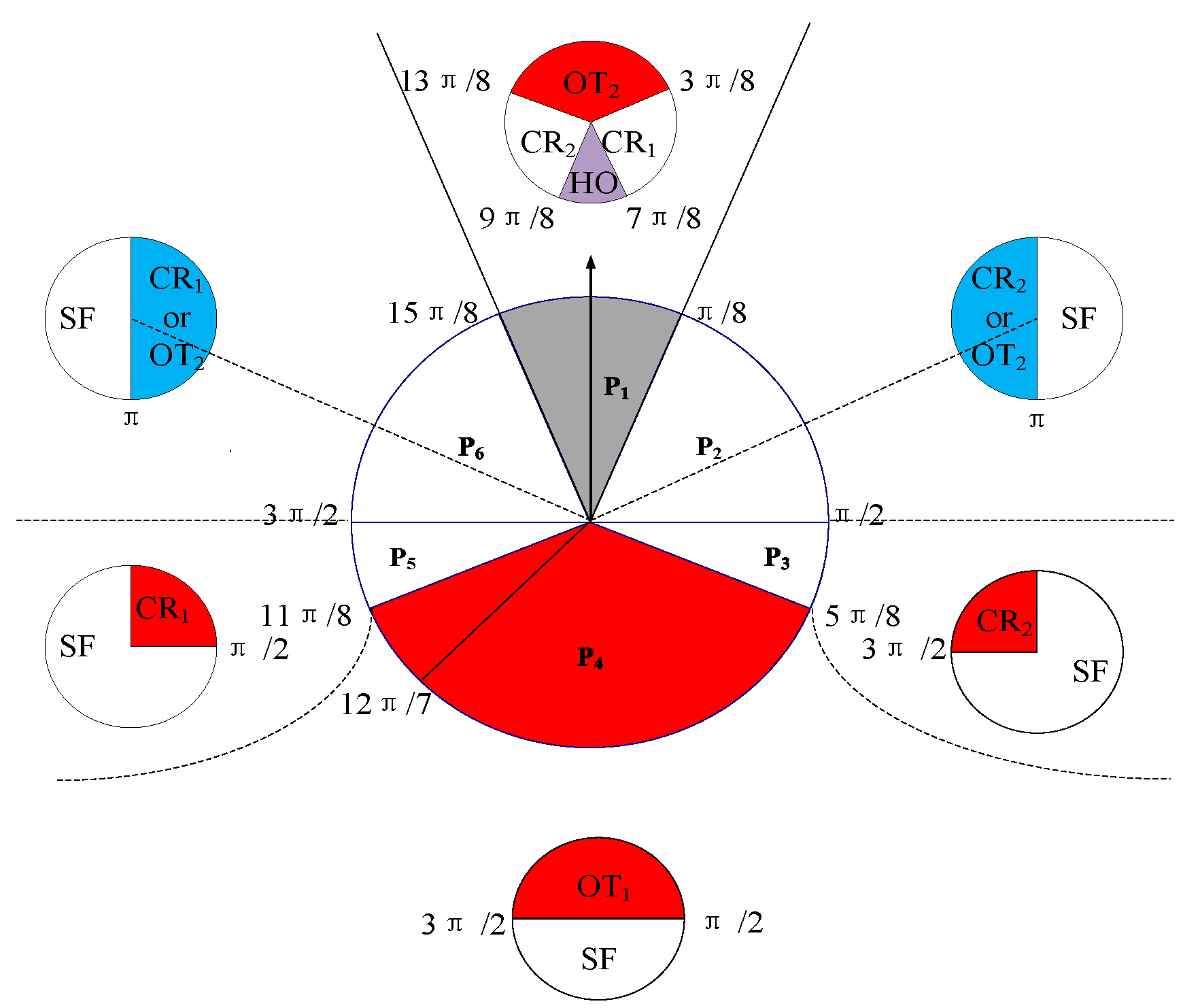
2.1. The Analysis of Encounter Situation

The encounter situation is a major and indispensable issue for collision avoidance since the obligation for the two parties takes effect when satisfying the requirements of the specific encounter situation [19]. However, there are different interpretations of the term ‘encounter situation’, though the exact definition is given in the COLREGs. For example, the applicable distance for which the various stages begin to apply varies considerably.
Currently, there are still no specialized reports on encounter situations except in research on the autonomy of ships. For example, the encounter situation is further divided into six types (crossing from the port/right side, overtaking, overtaken, head-on, and target ship with no speed) for the expert system [20]. Based on a survey of the navigators’ perception of the encounter situation, the boundary line for the three encounter situations is obtained by applying the method of fuzzy statistics [21]. Considering the determination of encounters by a single factor, the combined factors, including relative bearing, crossing angle, and speed, are applied to further divide the crossing situation into a large/small angle port/right side encounter [22]. Considering the consistency of the collision-avoidance actions, the recommended distinguishable relative bearing angles between head-on and crossing situations is enlarged [23].
In this article, the following principles for the division of encounter situations should be considered.
(1)
The division is based on the COLREGs, the navigator’s practical practice, and good seamanship.
(2)
All types of encounter situations are completely divided, and every encounter that needs to take collision avoidance actions can find corresponding encounter situations to guide collision avoidance behaviour.
(3)
The quantitative judgement results for each encounter situation should be unique.
(4)
Full accounts should be taken of the incompatibility between the two ships in their understanding and action of the situation.

2.1.1. The Quantified Criteria of Encounter Situations

Some assumptions are made to perform the determination of encounter situations. The ship domain is treated as circle, and the collision risk borrows the concept of ship domain by comparing the distance to the closest point of approach (DCPA) with the radius of ship domain Ds, whose radius is a statistical result in the open sea [24]. The applicable distance for a specific encounter situation is based on the visibility of lights for ships with lengths larger than 50 m.
First, the orientation division of the target ship (TS) is illustrated in Figure 1. The orientation division of the TS is categorized into six regions (P1, P2, P3, P4, P5, and P6). The corresponding values of the bearing lines taken clockwise are [π/8, π/2, 5π/8, 11π/8, 3π/2, and 15π/8], respectively, and are mainly based on the provision of the light’s arc of horizon defined in the COLREGs. The description of every possible encounter situation is listed in Table 1. In terms of legal status, only one ship needs to perform the evasive manoeuvre in a crossing situation, while both ships must perform evasive manoeuvres in a head-on situation according to Rule 14(c), ‘when a vessel is in any doubt as to whether such a situation exists she shall assume that it does exist and act accordingly’, the head-on section values (angles of π/8 radians) are larger than those recommended. Therefore, the enlarged section P1 reduces the sensitivity upon small changes in the own ship’s (OS) heading when changing HO to either GW or SO. To reduce the complexity of the procedure, the quantified criteria for specific encounter situations are clearly described in Table 2, and are based on the COLREGs, navigational practices, and good seamanship. The quantified criteria are established from the aspects of crossing angle, relative bearing, collision risk, and applicable distance for different encounters.

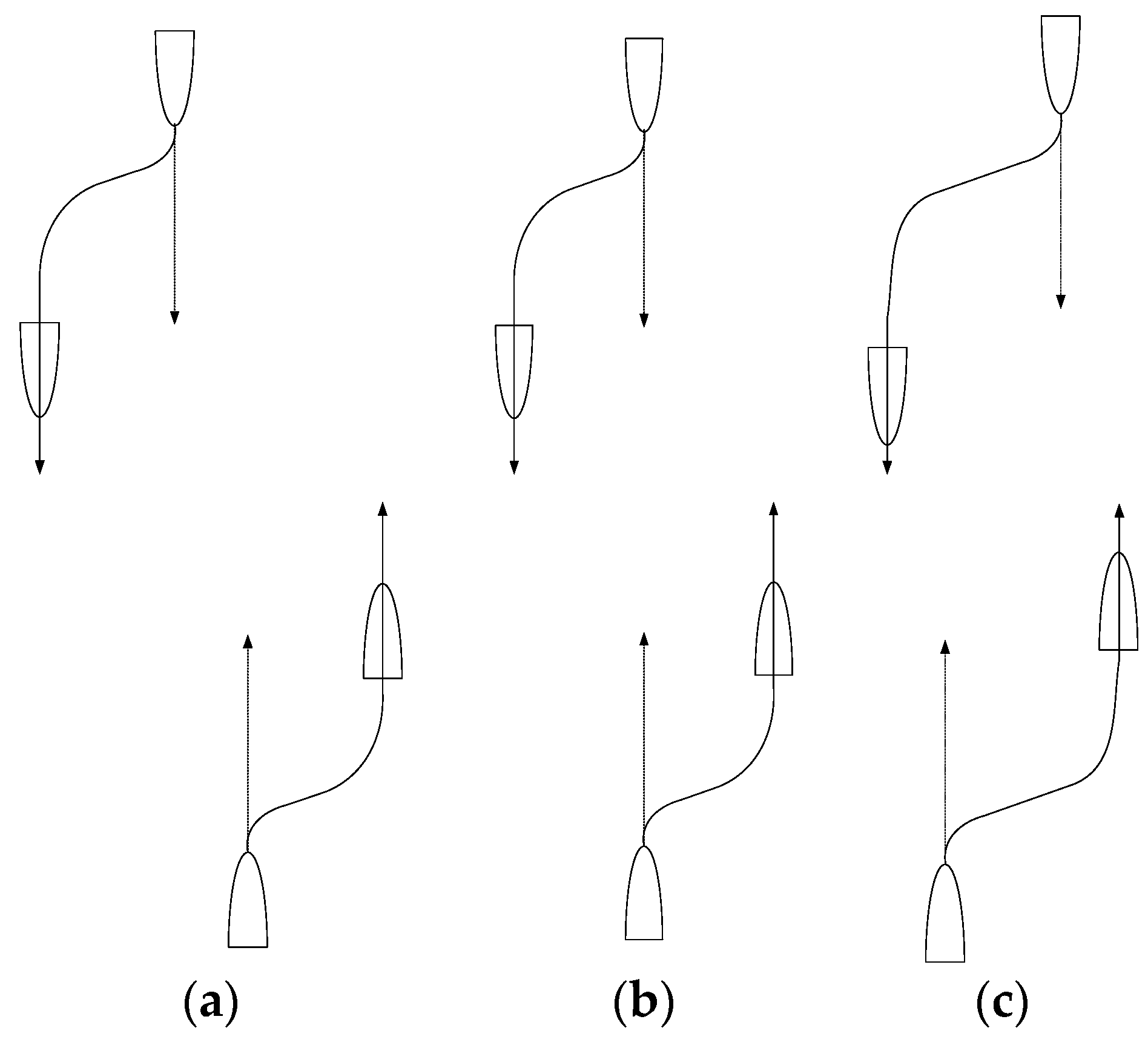
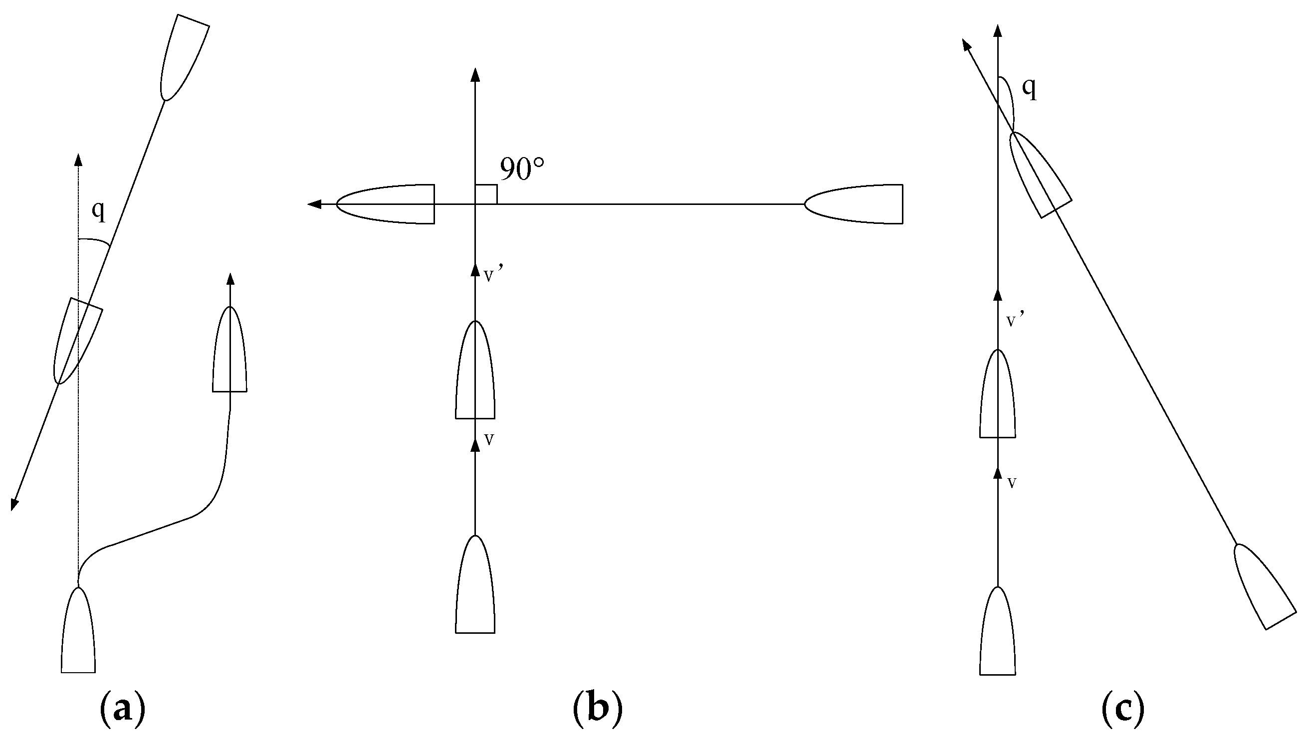
2.1.2. The Action Manner

To ensure that the evasive action complies with navigational practice. The action manner is mainly analysed based on COLREGs, good seamanship, and the cost of avoidance. The results are presented in Figure 2, Figure 3 and Figure 4. For a head-on situation, the action manner is an alteration of course to starboard regardless of a port-to-port encounter or a right-to-right encounter. For a crossing situation, usually a give-way vessel may keep clear of the other in the following ways: (1) For a small angle crossing angle, by altering course to right to cross stern of the give-way vessel; (2) for a right angle crossing situation, either by reducing speed or altering course to right to make other vessel cross ahead; (3) for a large angle crossing situation, by reducing speed to make the other vessel cross ahead. For an overtaking situation, the action manner is based on the bearing angle and the DCPA symbol (Zheng, 2000). (1) If DCPA > 0 and θT∈ [7π/6, 11π/8], the overtaking vessel alters course to starboard; (2) if DCPA ≤ 0 and θT∈ [7π/6, 11π/8] or the two ships heading in parallel, the overtaking vessel alters course to port; (3) if DCPA < 0 and θT∈ [5π/8, 7π/6], the overtaking vessel alters course to port; (4) if DCPA ≥ 0 and θT∈ [5π/8, 7π/6] or the two ships are heading in parallel, the overtaking vessel alters course to starboard.

2.2. Ship Manoeuvrability Model

Accurate and reliable simulation system for ship navigation requires precise knowledge of the manoeuvring behaviour of the ship no matter whether taking the manner of course alteration or speed reduction. In order to represent a manoeuvring ship fully in space, a mathematical model with six degrees of freedom is required. To simplify the problem, it is assumed that the steering of a ship can be regarded as a rigid body motion on the horizontal plane, as is customary.

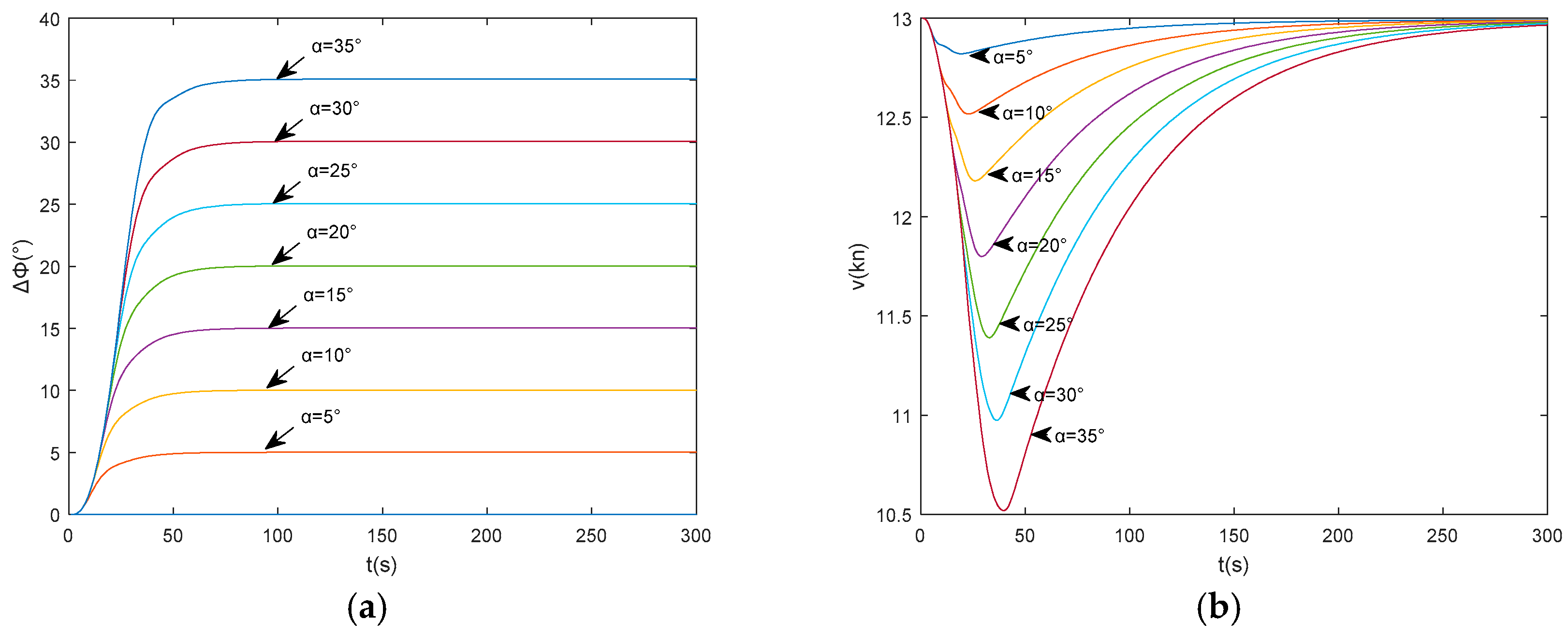
2.2.1. The Manoeuvre of Course Alteration

The transfer function of a ship as a course control object can be defined in a simplified form as a first-order Nomoto model. The relationship between the rudder angle δ and the ship’s heading angle ϕ is expressed as follows [25]:
ϕ + 1 T H ( ϕ · ) = K T δ
where K is the steering quality index, and T is the steering quality time constant.
The nonlinear function of H ( ϕ · ) with respect to ϕ · can be approximately represented by:
H ( ϕ · ) = a 1 ϕ · + a 2 ϕ + a 3 ϕ +
where ai (i = 1, 2, 3, …) is the nonlinear constant coefficients.
The velocity of the ship’s manoeuvring function can be expressed as follows [26]:
V · + a v v V 2 + a r r ϕ · 2 + a δ δ V 2 δ 2 = a n n n D 2 + a n v n D V
where n D is the rational speed of the main engine, V is the velocity, ann and anv are the propulsive coefficients, and avv, arr, and aδδ are the damping coefficients.
These coefficients can be expressed as follows:
a v v = 1 L a v v = 1 L X v v ( m + m x )
a n n = L a n n = L 2 C 1 ( m + m x ) ( D L ) 3 ( D d )
a r r = L a r r = l p ( m + c m m y ) ( m + m x )
a n v = a n v = 2 C 2 ( m + m x ) ( D L ) 2 ( D d )
a δ δ = 1 L a δ δ = 1 L X δ δ ( m + m x ) ( A R L d )
where L is the overall length, d is the draft, D is the diameter of the propeller, AR is the rudder area, lp is the distance between the gravity and pivoting point, cm is equivalent to the block coefficient of hull cb, C1 and C2 are the dimensionless values of effective thrust, and m, mx, and my are the dimensionless values of mass, longitudinal added mass, and lateral added mass, respectively.
The parameters m, mx, my, Xvv, and Xδδ are determined as follows:
m = 2 m ρ L 2 d
m x , y = 2 m x , y ρ L 2 d
X v v = 2 R t ρ v ) V 2
X δ δ = f α ( λ ) ( U R e o V ) 2
where ρ is the density of water, Rt represents the resistance of stable directional voyage, UReo represents the effective inflow speed of the rudder, and fα (λ) represents the nominal force gradient against the attack angle in the open sea.
The characteristics of the steering engine described in Equation (17) should not be ignored.
δ · = 1 T E δ + K E T E δ E
where δE is the rudder command angel, δ is the actual rudder angle, and TE and KE are the time constant and gain control of the steering engine, respectively. The maximum rudder angle should be smaller than 35°.
In this paper, a proportional-integral-derivative (PID)controller is adopted to control the ship’s heading. A PID controller attempts to correct the error between a measured process variable and a desired point by calculating and then outputting a corrective action that adjust the process accordingly. The rudder angle δE is controlled based on the heading error e = ϕrϕ, and ϕr is the desired heading angle, as expressed in Equation (18).
δ E = K p e + K d e · + K i e d t
where Kp is the proportional gain constant, Kd is the derivative time constant, and Ki is the integral time constant. The controller gains can be derived by pole placement using the design parameters ω n and ζ as follows:
K p = T ω 2 n K ,   K d = 1.8 ς . ω n 1 K ,   K i = ω 3 n T 10 K
where ω n is the natural frequency and ζ is the relative damping ratio of the first order system.
The implementation of the ship’s course control in the safe trajectory determination algorithm is manipulated by a PID controller. For a specific value of the ship’s speed, a family of characteristics showing the relationships of the manoeuvre time as a function of course and speed for different desired heading changing values is introduced in Figure 5. The corresponding heading angle value and speed value over manoeuvre time are saved and stored in a table and are read from the table for the fitness evaluation.

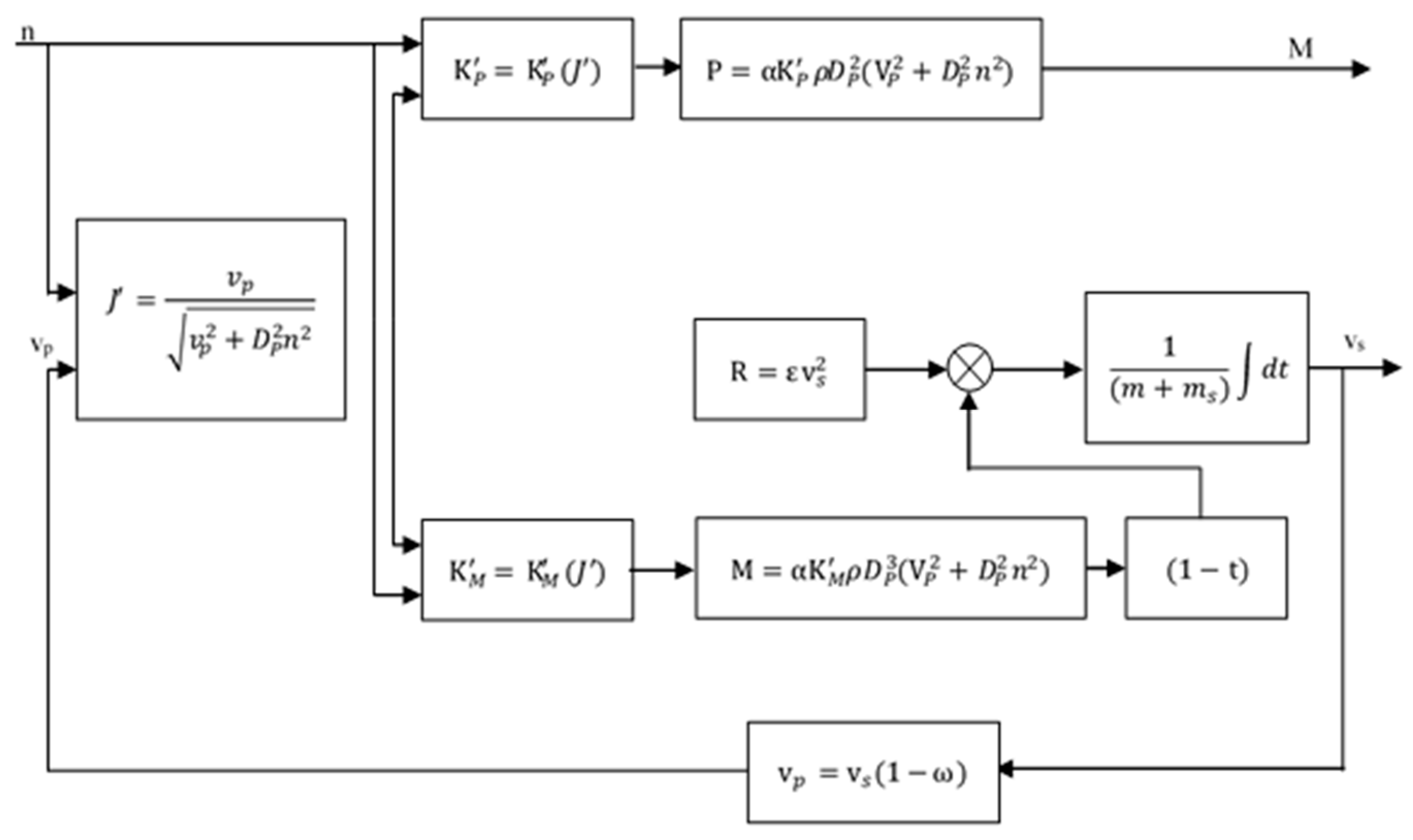
2.2.2. The Manoeuvre of Speed Reduction

The ship’s motion mathematical model of MMG, including the forces and moments acting upon the ship’s hull, propeller rudder and the interactions within them, is used to simulate the ship’s actual movement in various sea conditions. Considering the thrust deduction coefficient and wake coefficient, the expression is given as follows [27]:
Z p P ( 1 t ) R = ( m + m s ) d V s d t
P = K P ρ n 2 D 4
R r = ε v s 2
M = K M ρ n 2 D 5
K P = K P ( J )
K M = K M ( J )
J = v s ( 1 ω ) n D
where Zp is the number of propellers, ms is the additional mass, m is the ship mass (kg), vs is the ship speed relative to water (m/s), t is the thrust reduction coefficient, Rr is the ship resistance (N), P is the propeller thrust (N), M is the propeller torque (N.m), n is the propeller revolution speed (r/s), D is the propeller diameter (m), ρ is the water density (kg/m3), ω is the wake coefficient, Kp is the thrust coefficient, KM is the torque coefficient, and J is the advance coefficient.
In this article, the Wageningen B-screw series propellers chart is adopted, and the principal parameters of this series of propellers are disc-square ratio (A/Ad)0 = 0.45, blade number Z0 = 4, and patch ratio H/D = 0~1.6. As n approaches zero, J approaches infinity, which leads to data overflow in the computation [28]; thus, the expression is rewritten as follows:
J = v p / v p 2 + D P 2 n 2
v p = v s ( 1 ω )
P = α K P ρ D P 2 ( V P 2 + D P 2 n 2 )
M = α K M ρ D P 3 ( V P 2 + D P 2 n 2 )
α = Z 0 ( A / A d ) 0 / Z ( A / A d ) 3
where vp is propeller speed relative to water, α is the scaling factor, Z is the calculated blade number, and (A/Ad) is the calculated disk square ratio.
Generally, a function that is continuous can be expressed approximately as an n-order Chebyshev polynomial [29]. Then, the propeller thrust coefficient KP and torque coefficient KM about J’ can be obtained by Chebyshev polynomial fitting:
K P ( J ) = 1 2 a 0 P T 0 ( J ) + a 1 P T 1 ( J ) + a 2 P T 2 ( J ) + + a n P T n ( J )
K M ( J ) = a 0 M T 0 ( J ) + a 1 M T 1 ( J ) + a 2 M T 2 ( J ) + + a n M T n ( J )
where T0(J’) = 1, T1(J’) = J’, T2(J’) = 2J2-1, T3(J’) = 4J3−3J’…., the general recursive formula for Tk(J’) is Tk + 1(J’) −2JTk(J’) + Tk-1(J’) = 0 (k = 1,2,…n). The Chebyshev polynomial has the following features. First, the polynomial coefficients are independent of the order number n. Second, the fitting error is small, and the fitting result with finite order number n is the best approximation, meaning that the mean square error is the minimum. Finally, it is convenient to change from a given Chebyshev polynomial expression into ordinary polynomial.
There are two inertia subsystems in the ship-propeller system: Propeller rotation and ship translation. Translations of the thrust and torque within the two subsystems and their motions are interactive. The block diagram of the ship-propeller model is shown in Figure 6 [30].
The implementation of the ship’s speed control in the safe trajectory determination algorithm is realized by the ship-engine system. For a specific value of the ship’s propeller revolution, a family of characteristics showing the relationships of the manoeuvre time as a function of different desired revolution changing values is introduced in Figure 7.

2.3. Trajectory Planning for Collision Avoidance

Following the above-mentioned scheme, the encounter situation and the manner of evasive manoeuvre are determined. Then, the next focus is the trajectory planning to keep all the ships clear of the OS ship’s domain all the time. The complete collision-avoidance process incorporates the action of collision avoidance and restoration to the original trajectory.

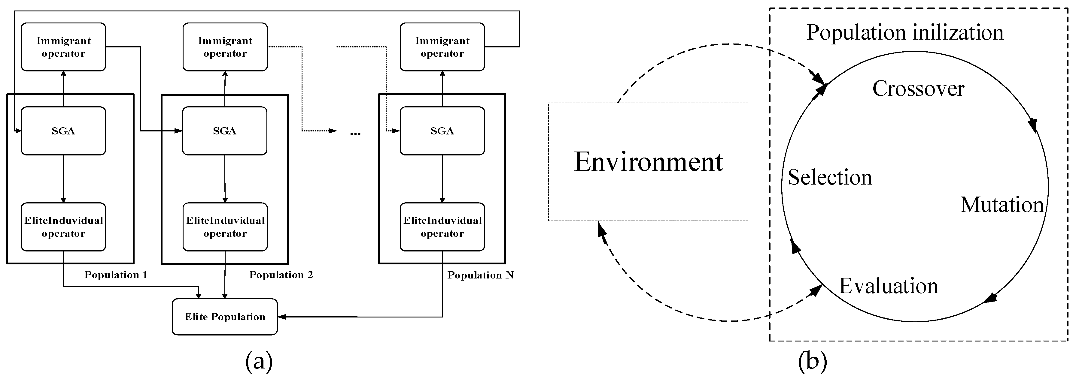
2.3.1. Multiple Genetic Algorithm

Considering the manner of course alteration, the speed and velocity change simultaneously, so the optimization has to deal with multiple variables. The Multiple Genetic Algorithm (MPGA) illustrated in Figure 8a is adopted to overcome the deficiency of Single Genetic Algorithm (SGA) in the aspects of premature convergence, local optimization ability, and parameter settings of genetic operators. The populations with different combinations of parameter settings of genetic operators are closely interwoven by the establishment of an immigrant operator, and the main idea is that the worst chromosome in any population is replaced by the best chromosome in the adjacent population to achieve co-evolution. By establishing an elite-individual operator, the individuals with lower fitness will be chosen to enter the elite population so that the superior individuals will not be lost, making it possible to find the global optimal solution. It is noticeable that the elite population does not perform selection, crossover, or mutation operation to ensure the integrity of the best individuals. The main difference between this algorithm and the MPGA used in [18], is that the evolutionary order of SGA phases shown in Figure 8b is adjusted here to improve the optimization efficiency. The crossover and mutation operators precede evaluation and selection instead of following them. The population size is tripled, then all the individuals in the expanded two population could be sufficiently crossed with each other due to the communication scheme. This change allows for sufficiently taking advantage of the local searching ability and preparing for the tournament selection strategy. In addition, the important change concerns population initialization. Apart from randomly generated individuals, the initial population is generated by a heuristic method (satisfying the constraints for course alteration based on COLREGs). Meanwhile, the evolutionary results of relevant genetic operations are also adjusted to keep the consistency of the optimal solution.

Encoding Technique

In this article, a real number encoding method is employed. Each gene is substituted with a desired course change value between adjacent turning points, as shown in Figure 9. In addition, the direction of course alteration is assumed as follows. If △ ϕ i > 0 , the give-way ship turns right, otherwise, the give-way ship turns left. This encoding technique is applied to fit the PID controller.

Constraint Conditions

To generate satisfactory trajectory compliance with the COLREGs and good seamanship, some constraints are set as follows. First, the direction of the course alteration is determined in Section 2.1.2. According to Rule 8(b), ‘any alteration of course and/or speed to avoid collision shall, if the circumstances of the case allow, be large enough to be readily apparent to another vessel observing visually or by radar’, therefore, the course alteration angle should be larger than 15° and smaller than π/3 to ensure the evasive manoeuvre is kept obvious [7]. It should be remarkable that the course alteration angle of the last gene is larger than 5° in order to guarantee the restoration to the initial track.
Δ ϕ i { | Δ ϕ 1 | = π 6 π 12 < | Δ ϕ i | π 6 ( i = 2 , 3 , , N 1 ) | Δ ϕ M | π 36 × k ( k Z + )

Fitness Function Model

The fitness function of a chromosome measures the cost of the trajectory it represents. As for the two-ship encounter, the function should consider three different optimisation factors: (1) Satisfy the clearance requirements, (2) maintain a smooth trajectory, and (3) guarantee less distance travelled; a linear combination of these factors is shown Equation (25).
= { α D e + 1000 D t D t < D s α D e + β ( D t D s ) D t > D s
D e = ( x n k x n k ) 2 + ( y n k y n k ) 2   ( i = 0 ,   1 ,   2 ,   3 , n ,   j = 1 ,   2 ,   3 ,   N )
D t = min ( ( x i j + 1 x i j ) 2 + ( y i j + 1 y i j ) 2
N 2 = min ( L V j × T × N 3 )
where { ( x i j ,   y i j ) | i = 1 ,   2 ,   3 , , n ,   j = 1 ,   2 ,   3 , , N } is two-dimensional coordinate arrays that record the optimal trajectories of all the ships, N is the number of encountering ships, assume ship k is the give-way ship, ( x i k ,   y i k ) is the planned trajectory of ship k, De is the destination deviation between the optimal trajectory and the planned route of the give-way ship, Dt is the minimum distance during the movement between any two ships, α and β are weight coefficient and n is determined by the time step T, the number of turning points, the segment step L, as well as the corresponding ship’s velocity.

2.3.2. Linear Extension Algorithm

For the manner of speed reduction, considering that the course remains unchanged, the linear extension method is adopted to determine the reduced revolution ratio and the corresponding duration. The main idea is determine the appropriate propeller revolution as well as restoration time. It is structured as shown in the pseudocode below. The propeller revolution is decreased by a fixed value in each loop until the give-way vessel can keep away from the stand-on vessels. The corresponding speed variation curve is obtained by the ship-engine model in Section 2.2.2. It should be noted that in the algorithm, a lower bound of half of a revolution, is set to avoid reducing the speed impracticably. When the give-way vessel passes the closest point of approach (CPA), the propeller rate of revolution restores to the original state.
1
V = VO: OS’s initial speed corresponding propeller revolution speed n = ne
2
n = n−Δn: Δn is a fixed value
3
Obtain the velocity variation curve;
4
Compute the minimum distance D t and the corresponding time tmin;
5
While DCPA < Ds and V ≥ 0.5VO
6
n = n−Δn;
7
End
8
If ttmin
9
nne: The propeller revolution restores to the initial state
10
End

3. Simulation Results and Analysis

The ship manoeuvrability-based simulation for ship navigation is tested on various typical traffic scenarios emulating different types of encounter situations. The determination of the encounter situation is based on the quantified criteria in Section 2.1.1. Then, the action manner by course alteration or reducing speed to perform collision avoidance is confirmed in Section 2.1.2. Finally, the corresponding trajectory planning model is activated. The dynamic property of a ship is considered in the process of collision avoidance. The initial traffic configurations are given in Table 3. Among them, the DCPA is the distance under the state without taking any collision avoidance measures. The simulation adopts the two exemplary ships with the principal dimensions shown in Table 4 and Table 5.
After careful consideration of the traffic scenarios for collision avoidance, the relevant parameters of the algorithm are set as follows: Group size, 100; crossover rate, 0.6; mutation rate, 0.04; and termination condition, 50. The parameters α and β in the fitness function model are 0.6 and 0.4, respectively. The simulation tests are run on a computer with a 2.5 GHz processor and 4 GB memory. When the optimal fitness value achieves convergence, or after it reaches the termination condition, the search is terminated, indicating that the optimal trajectory is supposedly found.
In fact, these tests primarily evaluate this simulation system’s performance in terms of effectiveness, consistency, and practicality. The simulation for each traffic scenario is run five times, and the corresponding optimal solutions are recorded in Table 6, Table 7, Table 8 and Table 9. In the figures showing the initial traffic configuration and the optimal trajectory, each vessel is colour coded, and the numbers on each position indicate the corresponding time in minutes. The blue line indicates the trajectory of ship B; the red line indicates the optimal trajectory of ship A; the red dotted line indicates ship A’s original track; and the black line represents the optimal trajectory of ship A without considering the ship manoeuvrability. Moreover, the variation curves of relative distance, velocity, and rudder angle are also illustrated. The radius of the ship’s domain is the safety criterion.

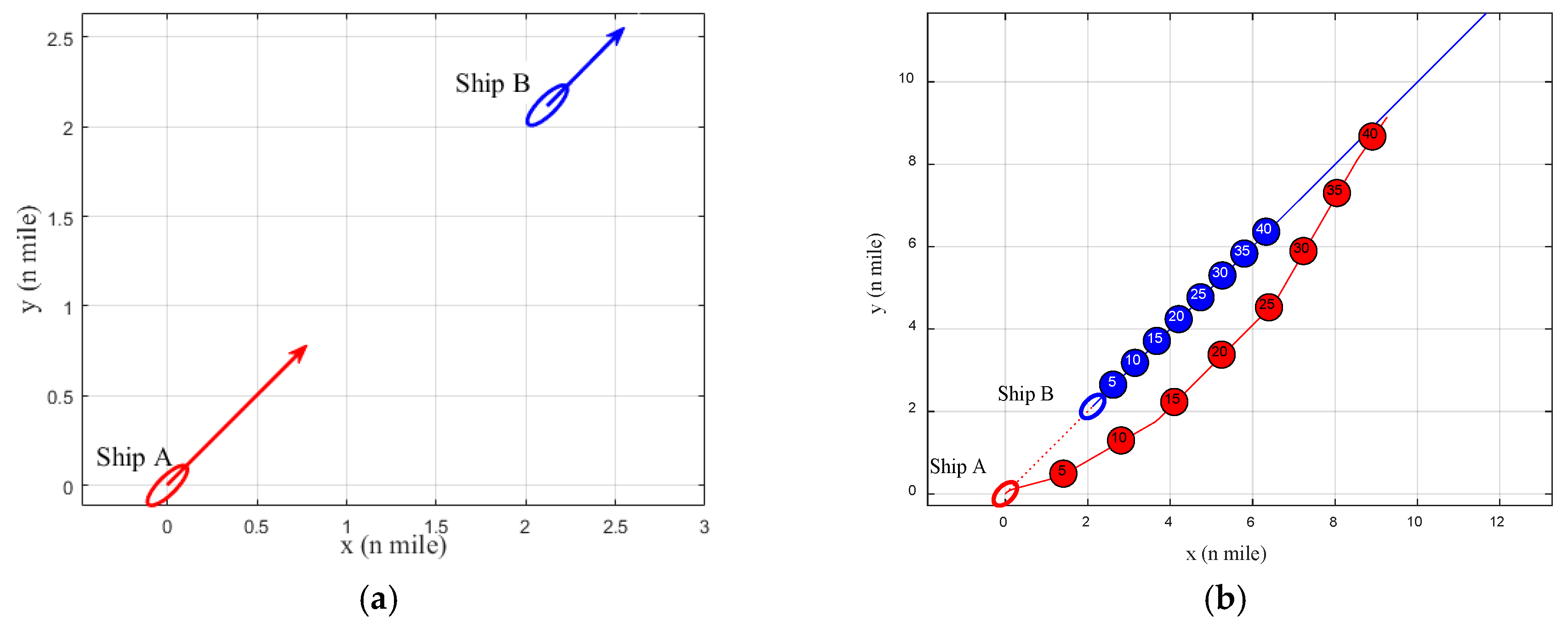
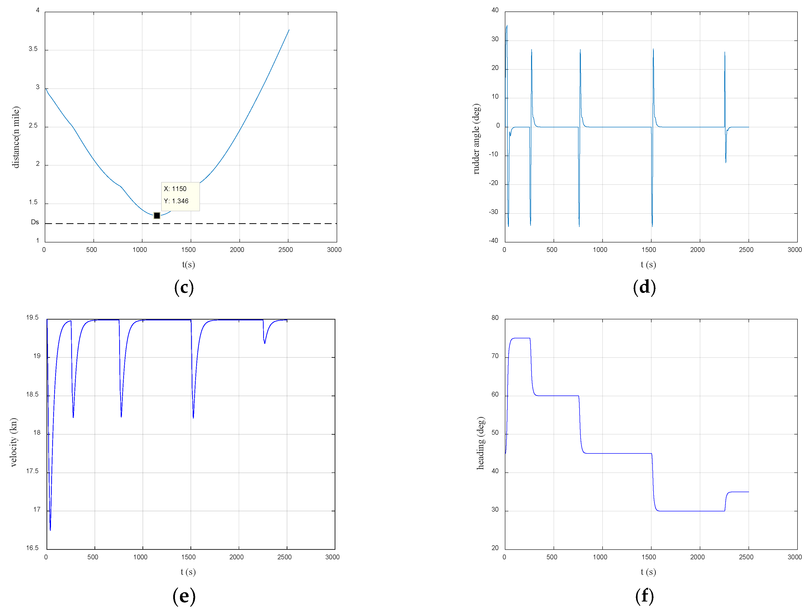
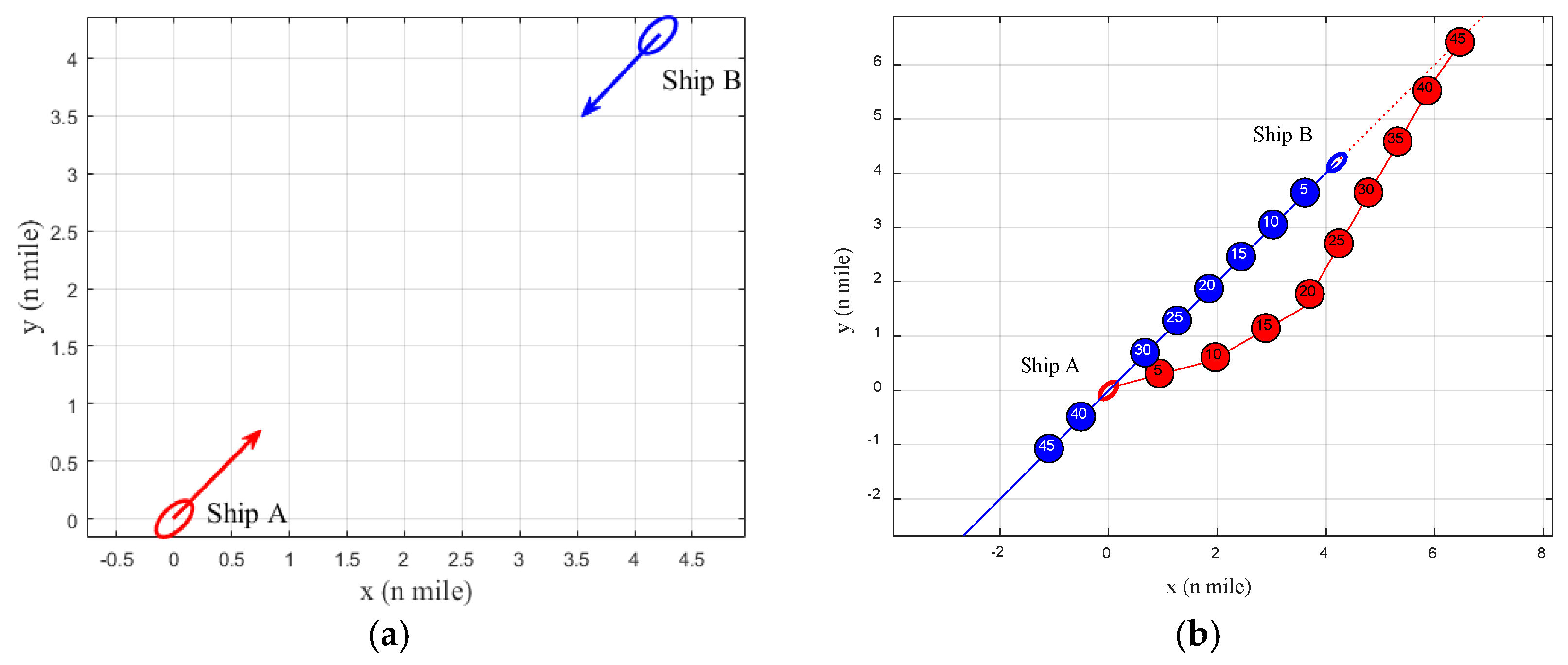
3.1. Case I: Head-On Situation

As seen from the initial traffic status illustrated in Figure 10a, ship A and ship B move on a reciprocal heading. According to the quantified criteria in Table 2, the relevant parameters are compared and analysed as follows: Ship B is in the region P1 of ship A (θB = 0∈ [0, π/8] ∪ [15π/8,2π]). As these two ships approach each other, the ship domain is violated, and risk of navigation collision occurs (DCPA = 0 n mile). Meanwhile, the criteria of crossing angle and applicable distance also satisfy the requirement of HO (CT = π∈ [7/π8,9π/8], R ≤ 6 n mile). Therefore, the encounter can be identified as a head-on situation in which the ships should pass each other port to port according to Rule 14 of the COLREGs. However, this simulation only calculates the trajectory of ship A as it is viewed from the perspective of ship A, which has already ensured safe navigation. Conversely, the evasive manoeuvre of ship B is also calculated from the point of ship B, while assuming ship A is the stand-on vessel.

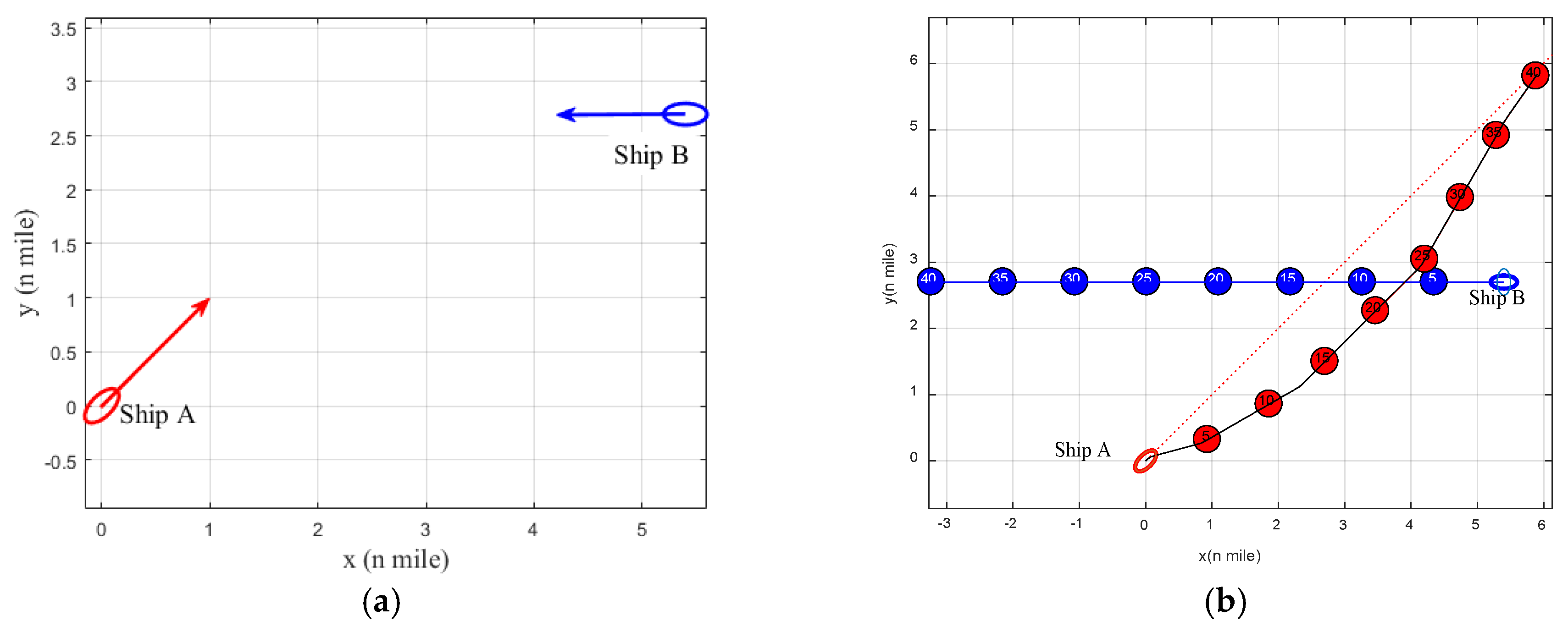
3.2. Case II: Small Angle Crossing Situation

As seen from the initial traffic status illustrated in Figure 11a, ship B is positioned before the starboard beam of ship A and the corresponding trajectories cross each other. According to the quantified criteria in Table 2, the relevant parameters are compared and analysed as follows: Ship B is also in the region P1 of ship A (θB = 18.4° ∈ [0,π/8] ∪ [15π/8,2π]) As these two ships approach each other, the ship domain is violated, and risk of navigational collision occurs (DCPA = 0.52 n mile). Meanwhile, the criteria of crossing angle and applicable distance also satisfy the requirement of CR2 (CT = 225° ∈ [9π/8,13π/8], R ≤ 6 n mile. As a consequence, it allows us to evaluate the collision risk in Rule 15 of the COLREGs for a small angle crossing situation. Based on the analysis for the action manner in Section 2.1.2, it is compliant with the situation in Figure 3a so that ship A should alter course to starboard to pass the stern of ship B.

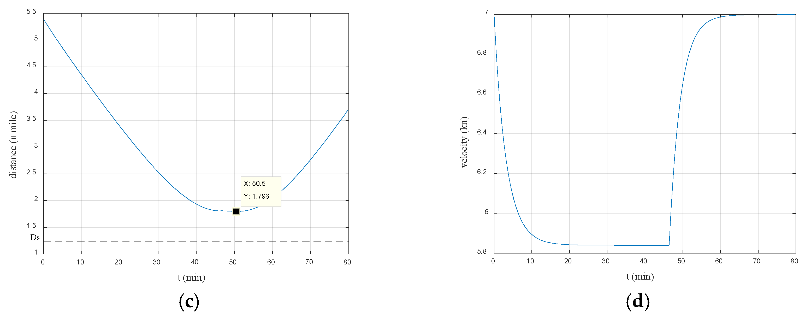
3.3. Case III: Overtaking Situation

As seen in the initial traffic status illustrated in Figure 12a, ship A is in the stern of ship B. The relevant parameters are compared and analysed as follows: Ship A is in region P2 of ship B (θA = 180° ∈ [5π/8,11π/8]). As these two ships approach each other, the ship domain is violated, and risk of navigation collision occurs (DCPA = 0.19 n mile). Meanwhile, the criteria of crossing angle and applicable distance still satisfy the requirement of CR2 (CT = 0° ∈0, π/2 ∪ [3π/2,2π], R ≤ 6 n mile). Therefore, it allows us to evaluate the collision risk in Rule 15 of the COLREGs for an overtaking situation. Based on the analysis for the action manner in Section 2.1.2, it is compliant with the situation in Figure 4e in which ship A should alter course to starboard to overtake ship B.

3.4. Case IV: Large Angle Crossing Situation

As seen in the initial traffic status illustrated in Figure 13a, ship B is also positioned before the starboard beam of the ship, and the corresponding trajectories cross each other. Similarly, the relevant parameters are compared and analysed as follows: Ship A is in region P2 of ship B (θA = 23.2° ∈ [π/8, π/2]. As these two ships approach each other, the ship domain is violated, and risk of navigational collision occurs (DCPA = 0.19 n mile). Meanwhile, the criteria of crossing angle, and the relative bearing of ship B with respect to ship A together with the applicable distance still satisfy the requirement of CR2 (CT = 330° ∈ [π,2π], θB = 233.2° < 11π/8, R ≤ 6 n mile). Therefore, it allows us to evaluate the collision risk in Rule 13 of the COLREGs for a small angle crossing situation. Based on the analysis for the action manner in Section 2.1.2, it is compliant with the situation of Figure 3c in which ship B should reduce speed to pass the stern of ship A.

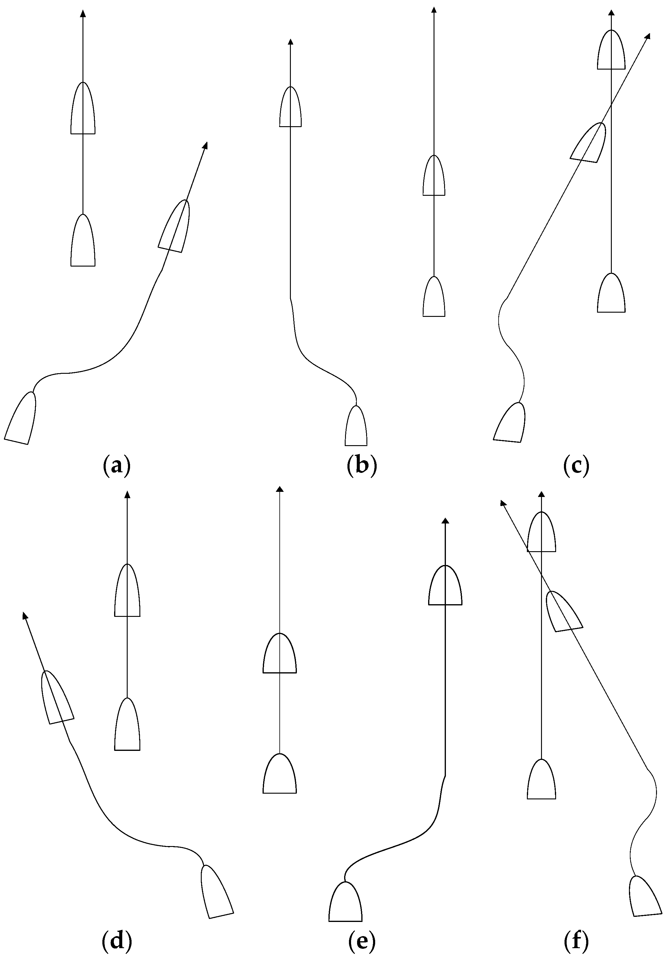
3.5. Analysis and Discussion

For cases I, II, and III, the give-way vessel takes evasive manoeuvres by altering course. The simulation results remain unchanged, as illustrated in Table 6, Table 7 and Table 8, due to the fixed distance step and the altering angle constraints in the algorithm. To intuitively demonstrate the simulation of ship navigation, Figure 10, Figure 11 and Figure 12b show the optimal trajectory marked by different coloured circles; the numbers on each position indicate the corresponding time in minutes. The closest point of approach (CPA) is larger than the safety criterion, which are both clearly marked in Figure 10, Figure 11 and Figure 12c. Figure 10, Figure 11 and Figure 12d–e give the curves of the rudder angle and velocity in the process of collision avoidance. Figure 10, Figure 11 and Figure 12f show the good tracking performance for the give-way ship’s heading angle relative to the desired heading, which reflects the manoeuvring characteristic of ship motion and control, such as inertia and nonlinear. For case IV, the give-way vessel takes action by changing speed. The optimal solution also remains unchanged for a specific encounter situation because the fixed revolution reduction ratio is adopted shown in Table 9. However, the final CPA is much larger than the safety criteria illustrated in Figure 13c because this algorithm lowers the standard in terms of trajectory length in order to guarantee that the optimal solution is more practical. In fact, there are mainly two reasons including the adoption of the fixed reduced revolution ratio and the restoration time influencing the distance variation between ships. The more elaborate division of the fixed revolution reduction ratio, the greater closeness of CPA, and the safety criteria. This would increase the computation time and make no sense. In this article, the restoration time is when the give-way vessel passes the closet distance point CPA of the first speed-reducing action. If the restoration time is before the corresponding tmin just to make the trajectory length relatively short, it will result in the phenomenon that the give-way vessel speeds up to approach the stand-on vessel in the process of collision, which would lay a heavy burden on the navigator of the stand-on vessel. The other simulation results, including the optimal trajectory and velocity variation curves, are presented in Figure 13b,d. The planned trajectory of the give-way vessel is also marked by a green circle to compare it with the optimal trajectory. The density of the circle reflects the process of acceleration and deceleration.
From the simulation results, some conclusions can be drawn. The effectiveness of this simulation for ship navigation in collision situations is mainly reflected in two aspects. One is that the optimal trajectories in different traffic scenarios contain intact evasive manoeuvres, including the action of collision avoidance and the restoration to the original trajectory; the other is that the new CPAs exceed the safety criteria, i.e., the radius of the ship domain in the whole process of ship navigation. For the aspect of consistency demonstration, the avoidance obligation is certain as the encounter situation is derived from COLREGs from the perspective of either party. By adopting the fixed distance step, altering angle constraints as well as the fixed revolution reduction ratio in the algorithm, the optimal solutions could remain unchanged for the same input. Additionally, the action manner is determined based on the COLREGs, good seamanship, and cost of avoidance, which can reduce the doubt about the evasive manoeuvre to the greatest extent, especially in encounters between unmanned ships and manned ships. To demonstrate the practicality, the dynamic property of ship manoeuvring is considered in the process of collision avoidance to improve the reliability of the simulation system. More importantly, it is clear in the heading alteration curve that the evasive manoeuvres simulated by the multiple genetic algorithm are performed with fewer course deviations compared with the initial assumed number of turning points, which are compliant with navigational practice.

4. Conclusions

This paper has presented a method for automatic trajectory planning and collision avoidance for use in ship manoeuvrability-based simulation for ship navigation. Under the general requirements from the COLREGs and good seamanship, the determination of an encounter situation is quantified to reduce the intervention of navigators. Meanwhile, the action manner by course alteration or changing speed in some typical encounter situations is graphically analysed for both give-way and stand-on vessels to make the evasive action compliant with navigational practice and to reduce the doubt about the evasive manoeuvre, especially in encounters between unmanned ships and manned ships. By adopting the fixed distance step, altering angle constraints, and the fixed revolution reduction ratio in the algorithm, the optimal solution can remain unchanged for the same traffic scenario. More importantly, the mathematical model of ship motion and ship manoeuvring control mechanism is adopted, which can eliminate the insufficiency of neglect of ship manoeuvrability in the process of collision avoidance. Meanwhile, the course encoding technique is adopted to fit the ship manoeuvring control mechanism. Finally, a set of traffic scenarios simulating different encounter situations is applied to demonstrate the effectiveness consistency and practicality of this simulation system. However, since only the applicable distance for different encounter situations is analysed, the specific action time is not considered, and our future research will concentrate on the choice of action time, especially for multi-ship collision avoidance.

Author Contributions

S.N. conceived and performed the experiments; Z.L. and Y.C. supervised and designed the research and contributed to the article’s organization. S.N. drafted the manuscript, which was revised by all authors. All authors read and approved the final manuscript.

Funding

This work is supported by the National Natural Science Foundation of China (Grant 51309041).

Conflicts of Interest

The authors declare no conflict of interest.

Nomenclature

CTTS‘s heading crossing angle with respect to OSKiintegral time constant
θOOS’s relative bearing with respect to TS ω n natural frequency
θTTS’s relative bearing with respect to OSζrelative damping ratio
Dsradius of the ship domainZpnumber of propellers
Rdistance between OS and TS m, msship mass and additional mass
ϕOthe heading of own shipvsspeed relative to water
ϕTthe heading of target shipvppropeller speed relative to water
δrudder angletthrust reduction coefficient
Ksteering quality indexRrship resistance
Tsteering quality time constantPpropeller thrust
nDthe rational speed of main engineMpropeller torque
Loverall length of shipnpropeller revolution speed
ddraftDpropeller diameter
Ddiameter of the propellerωwake coefficient
ARrudder areaKPthrust coefficient
lpdistance between the gravity and pivoting pointKMtorque coefficient
cbblock coefficient of hullJadvance coefficient
m,
mx
my
dimensionless values of masslongitudinal added masslateral added massA/Addisc–square ratio
ρdensity of waterZblade number
Rtresistance of stable directional voyageH/Dpatch ratio
UReothe effective inflow speed of the rudderDedestination deviation between the optimal trajectory and the planned route of give-way ship
fα (λ)nominal force gradient against the attack angleDtminimum distance during the movement between any two ships
δErudder command angle α a weight coefficient indicating the deviation degree between the optimal trajectory and the planned route
TEtime constant β a weight coefficient indicating the risk of collision
KEgain control of the steering engineTtime step
ϕrdesired heading angle N 3 number of turning points
Kpproportional gain constantlsegment step
Kdderivative time constantnerational revolution of propeller

References

  1. Ahn, J.H.; Rhee, K.P.; You, Y.J. A study on the collision avoidance of a ship using neural networks and fuzzy logic. Appl. Ocean Res. 2012, 37, 162–173. [Google Scholar] [CrossRef]
  2. Kim, D.; Hirayama, K.; Okimoto, T. Distributed stochastic search algorithm for multi-ship encounter situations. J. Navig. 2017, 70, 1–20. [Google Scholar] [CrossRef]
  3. Lazarowska, A. Ship’s Trajectory planning for collision avoidance at sea based on ant colony optimization. J. Navig. 2015, 68, 291–307. [Google Scholar] [CrossRef]
  4. Naeem, W.; Irwin, G.W.; Yang, A. COLREGs-based collision avoidance strategies for unmanned surface vehicles. Mechatronics 2012, 22, 669–678. [Google Scholar] [CrossRef]
  5. Perera, L.P.; Carvalho, J.P.; Soares, C.G. Intelligent ocean navigation and fuzzy-bayesian decision action formulation. IEEE J. Ocean Eng. 2012, 37, 204–219. [Google Scholar] [CrossRef]
  6. Szlapczynski, R.; Szlapczynska, J. A method of determining and visualizing safe motion parameters of a ship navigating in restricted waters. Ocean Eng. 2017, 129, 363–373. [Google Scholar] [CrossRef]
  7. Tam, C.K.; Bucknall, R. Cooperative path planning algorithm for marine surface vessels. Ocean Eng. 2013, 57, 25–33. [Google Scholar] [CrossRef]
  8. Tsou, M.C. Multi-target collision avoidance route planning under an ECDIS framework. Ocean Eng. 2016, 121, 268–278. [Google Scholar] [CrossRef]
  9. Wang, X.; Liu, Z.J.; Cai, Y. The ship maneuverability based collision avoidance dynamic support system in close-quarters situations. Ocean Eng. 2018, 146, 486–497. [Google Scholar] [CrossRef]
  10. Zhang, J.; Zhang, D.; Yan, X.; Haugen, S.; Soares, C.G. A distributed anti-collision decision support formulation in multi-ship encounter situations under COLREGs. Ocean Eng. 2015, 105, 336–348. [Google Scholar] [CrossRef]
  11. The International Maritime Organization (IMO). Conventions on the International Regulations for Preventing Collision at Sea (COLREGs); The International Maritime Organization (IMO): London, UK, 1972. [Google Scholar]
  12. Sun, X.; Wang, G.; Fan, Y.; Mu, D.; Qiu, B. Collision avoidance using finite control set model predictive control for unmanned surface vehicle. Appl. Sci. 2018, 8, 926. [Google Scholar] [CrossRef]
  13. Lyu, H.; Yin, Y. COLREGS-Constrained Real-time Path Planning for Autonomous Ships Using Modified Artificial Potential Fields. J. Navig. 2018, 1–21. [Google Scholar] [CrossRef]
  14. Xue, Y.; Clelland, D.; Lee, B.S.; Han, D. Automatic simulation of ship navigation. Ocean Eng. 2011, 38, 2290–2305. [Google Scholar] [CrossRef]
  15. Wu, Z.L. Collision Avoidance and Watchkeeping, 2th ed.; Dalian Maritime University Press: Dalian, China, 2007. [Google Scholar]
  16. Campbell, S.; Naeem, W.; Irwin, G.W. A review on improving the autonomy of unmanned surface vehicles through intelligent collision avoidance manoeuvres. Annu. Rev. Control 2012, 36, 267–283. [Google Scholar] [CrossRef]
  17. Hong, B.G.; Yang, L.J. Ship Handling; Dalian Maritime University Press: Dalian, China, 2012. [Google Scholar]
  18. Ni, S.K.; Liu, Z.J.; Cai, Y.; Wang, X. Modelling of ship’s trajectory planning in collision situations by hybrid genetic algorithm. Pol. Marit. Res. 2018, 25, 14–25. [Google Scholar] [CrossRef]
  19. Cockcroft, A.N.; Lameijer, J.N.F. A Guide to the Collision Avoidance Rules, 4th ed.; Heinemann Newnes: Oxford, UK, 1990. [Google Scholar]
  20. Coenen, F.P.; Sneaton, G.P.; Bole, A.G. Knowledge based collision avoidance. J. Navig. 1980, 42, 107–116. [Google Scholar] [CrossRef]
  21. Zheng, Z.Y. Research on Automatic Decision-Making System of Vessel Collision Avoidance; Dalian Maritime University Press: Dalian, China, 2000. [Google Scholar]
  22. Weng, Y.Z. The knowledge about the field of preventing collisions and expert system. Navig. China 1994, 2, 45–50. [Google Scholar]
  23. Tam, C.K.; Bucknall, R. Collision risk assessment for ships. J. Mar. Sci. Technol. 2010, 15, 257–273. [Google Scholar] [CrossRef]
  24. Sun, L.C. The Research on Mathematic Models of Decision-Making in Ship Collision Avoidance; Dalian Maritime University Press: Dalian, China, 2000. [Google Scholar]
  25. Yang, Y.S.; Ren, J.S. Adaptive fuzzy robust tracking controller design via small gain approach and its application. IEEE Trans. Fuzzy Syst. 2003, 11, 783–795. [Google Scholar] [CrossRef]
  26. Yoshimura, Y.; Nomoto, K. Modeling of maneuvering behavior of ships with a propeller idling, boosting and reversing. J. Soc. Nav. Archit. Jpn. 1978, 144, 57–69. [Google Scholar] [CrossRef]
  27. Huang, H.; Shen, A.D.; Chu, J.X. Research on propeller dynamic load simulation system of electric propulsion ship. China Ocean Eng. 2013, 27, 255–263. [Google Scholar] [CrossRef]
  28. Zhang, W.J.; Tao, H.Y.; Zhu, Y.L. Modeling and dynamic simulation of the propulsion plant. Comput. Simul. 2002, 19, 88–90. (In Chinese) [Google Scholar]
  29. Li, D.P.; Wang, Z.Y.; Chi, H.H. Chebyshev fit of propeller properties across four quadrants and realization of all-round movement simulation along X-shift of DSV. J. Syst. Simul. 2002, 14, 935–938. (In Chinese) [Google Scholar]
  30. Shen, A.D.; Huang, X.W.; Zheng, H.Y.; Yang, X.L. Design of a semi-physical simulation system for electric podded propulsion. J. Yangzhou Univ. 2005, 8, 74–78. (In Chinese) [Google Scholar]
Figure 1. The orientation division of the target ship (TS) (the own ship (OS) is situated at the centre).
Jmse 07 00090 g001
Figure 2. The illustration of a head-on situation (a) port-to-port encounter, (b) meeting on reciprocal courses, and (c) right-to-right encounter.
Jmse 07 00090 g002
Figure 3. The illustration of a crossing situation (a) small angle crossing, (b) right angle crossing, and (c) large angle crossing.
Jmse 07 00090 g003
Figure 4. Overtaking situation (a) DCPA > 0 and θT∈ [7π/6, 11π/8], (b) θT∈ [7π/6, 11π/8] and ϕO = ϕT, (c) DCPA ≤ 0 and θT∈ [7π/6, 11π/8], (d) DCPA < 0 and θT∈ [5π/8, 7π/6], (e) θT∈ [5π/8, 7π/6] and ϕO = ϕT, and (f) DCPA ≥ 0 and θT∈ [5π8, 7π/6].
Jmse 07 00090 g004
Figure 5. The dynamic properties of a ship for different desired heading changing values. (a) The heading angle value over manoeuvre time; (b) the speed value over manoeuvre time.
Jmse 07 00090 g005
Figure 6. Diagram of the ship-propeller math model.
Jmse 07 00090 g006
Figure 7. The dynamic properties of a ship for different desired propeller revolution values.
Jmse 07 00090 g007
Figure 8. (a) The flow chart of multiple genetic algorithm; (b) The updated scheme of the Single Genetic Algorithm (SGA).
Jmse 07 00090 g008
Figure 9. The encoding method of chromosome.
Jmse 07 00090 g009
Figure 10. Simulation results for a head-on situation. (a) Initial traffic configuration; (b) optimal trajectory; (c) relative distance; (d) rudder angle of ship A; (e) velocity of ship A; and (f) heading of ship A.
Jmse 07 00090 g010aJmse 07 00090 g010b
Figure 11. Simulation results for a small crossing angle situation. (a) Initial traffic configuration; (b) optimal trajectory; (c) relative distance; (d) rudder angle of ship A; (e) velocity of ship A; and (f) heading of ship A.
Jmse 07 00090 g011aJmse 07 00090 g011b
Figure 12. Simulation results for overtaking situations. (a) Initial traffic configuration; (b) optimal trajectory; (c) relative distance; (d) rudder angle of ship A; (e) velocity of ship A; and (f) heading of ship A.
Jmse 07 00090 g012aJmse 07 00090 g012b
Figure 13. Simulation results for a large angle crossing situation. (a) Initial traffic configuration; (b) optimal trajectory; (c) relative distance; and (d) velocity of ship B.
Jmse 07 00090 g013aJmse 07 00090 g013b
Table 1. Abbreviations and brief descriptions of the encounter types.
AbbreviationsDescription
HOHead-on encounter when OS and TS give way simultaneously
OT1OS is overtaken by TS when TS gives way
OT2TS is overtaken by OS when OS gives way
CR1Crossing encounter when TS gives way
CR2Crossing encounter when OS gives way
SFSafe encounter
Table 2. The quantified criteria for specific encounter situations.
RegionHOCR1CR2OT1OT2
P1 θT∈ [0, π/8] ∪ [15π/8,2π]CT∈ [7π/8, 9π8] Ds ≤ DCPA
R ≤ 6 n mile
CT∈ [3π/8,7π8] Ds ≤ DCPA
R ≤ 6 n mile
CT∈ [9π/8,13π/8] Ds ≤ DCPA
R ≤6 n mile
---CT∈ [0,3π/8] ∪ [15π/8,2π] Ds ≤ DCPA
R ≤ 3 n mile
P2 θT∈ [π/8,π/2]----------CT∈ [π,2π] θO < 11/8π Ds ≤ DCPA
R ≤ 6 n mile
---CT∈ [π,2π] θO < 11/8π Ds ≤ DCPA
R ≤ 3 n mile
P3 θT∈[π/2,5π/8]------CT∈ [3π/2,2π] Ds ≤ DCPA R ≤ 6 n mile------
P4 θT∈ [5π/8,11π/8]---------CT∈ [0,2π] ∪ [3π2,2π] Ds ≤ DCPA R ≤ 3 n mile---
P5 θT∈[11π/8,3π/2] CT∈ [0, π/2]
Ds ≤ DCPA
R≤6n mile
P6 θT∈[3π/2,15π/8] CT∈ [0, π] θO < 5/8π Ds ≤ DCPA R ≤ 6 n mile CT∈ [0, π] θO > 5/8π Ds ≤ DCPA R ≤ 3 n mile
Safe encounter (SF) is not described in the table, as this encounter shares the same characteristic in which the parties move away from each other; C T is the heading crossing angle for TS with respect to OS; θO indicates OS’s relative bearing with respect to TS; θT is TS’s relative bearing with respect to OS; R is the distance between OS and TS; Ds is the radius of the ship domain.
Table 3. Ship encounter information for different scenarios.
ParametersCase ICase IICase IIICase IV
Position of ship A/n mile(0, 0)(0, 0)(0, 0)(5, −4)
Speed of ship A/n mile/h131319.513
Course of ship A/°454545330
Position of ship B/n mile(4.2, 4.2)(5.4, 2.7)(2.12, 2.12)(0, −6)
Speed of ship B /n mile/h1013913.6
Course of ship B/°225270450
DCPA00.5200.19
R5.96.03.05.4
Table 4. Principal particulars and manoeuvrability characteristics of ship A.
ParametersValueParametersValue
Length Overall/m126.0KE1
Breadth/m20.0TE2.5
Draft/m8.0avv1.4 × 10−4
Block coefficient0.681aδδ1.6 × 10⁻³
Displacement/ton14278arr101.5
N r/m120ann1.4 × 10−2
K0.48anv5.9 × 10−4
T216.5
Table 5. Main principal particulars of the ship-propeller model of ship B.
NameValueNameValue
Length overall/m189.99Propeller moment of inertia/kg × m322050
Draft/m6.0Propeller diameter/m5.85
Displacement/m327522Pitch ratio0.748
Rated speed/n mile/h13.6Area ratio0.558
Rated power of motor/kw7440Block coefficient0.7883
Propeller number1Diamond coefficient0.54
Propeller typeFixed pitchPropeller revolution speed/r × min−1108
Propeller blade number4Mass/kg14350
Table 6. Optimal solutions in a head-on situation.
Sequence∆ϕ1 (°)∆ϕ2 (°)∆ϕ3 (°)∆ϕ4 (°)∆ϕ5 (°)∆ϕ6 (°)∆ϕ7 (°)∆ϕ8 (°)∆ϕ9 (°)∆ϕ10 (°)
Solution 1300−150−3000005
Solution 2300−150−3000005
Solution 3300−150−3000005
Solution 4300−150−3000005
Solution 5300−150−3000005
Table 7. Optimal solutions in a small angle crossing situation.
Sequence∆ϕ1 (°)∆ϕ2 (°)∆ϕ3 (°)∆ϕ4 (°)∆ϕ5 (°)∆ϕ6 (°)∆ϕ7 (°)∆ϕ8 (°)∆ϕ9 (°)∆ϕ10 (°)
Solution 130−15−0−1500−15005
Solution 230−15−0−1500−15005
Solution 330−15−0−1500−15005
Solution 430−15−0−1500−15005
Solution 530−15−0−1500−15005
Table 8. Optimal solutions in an overtaking situation.
Sequence∆ϕ1 (°)∆ϕ2 (°)∆ϕ3 (°)∆ϕ4 (°)∆ϕ5 (°)∆ϕ6 (°)∆ϕ7 (°)∆ϕ8 (°)∆ϕ9 (°)∆ϕ10 (°)
Solution 130−15−0−1500−15005
Solution 230−15−0−1500−15005
Solution 330−15−0−1500−15005
Solution 430−15−0−1500−15005
Solution 530−15−0−1500−15005
Table 9. Optimal solutions in a large angle crossing situation.
SequenceInitial Revolution (r/s)Initial Velocity (n Mile/h)Reduced Revolution (r/s)The Reduced Velocity (n Mile/h)Period of Staying on the New Revolution (s)
Solution 11.813.60.31.162785
Solution 21.813.60.31.162785
Solution 31.813.60.31.162785
Solution 41.813.60.31.162785
Solution 51.813.60.31.162785

