Modeling Sediment Bypassing around Idealized Rocky Headlands
by
 , , , and
Douglas A. George
1,*, 
John L. Largier
1,
Gregory Brian Pasternack
2,
Patrick L. Barnard
3,
Curt D. Storlazzi
3 and
Li H. Erikson
3 1
University of California, Davis, P.O. Box 247, Bodega Bay, CA 94923, USA
2
Department of Hydrologic Sciences, University of California, Davis, One Shields Avenue, Davis, CA 95616, USA
3
Pacific Coastal and Marine Science Center, United States Geological Survey, Santa Cruz, CA 95060, USA
*
Author to whom correspondence should be addressed.
J. Mar. Sci. Eng. 2019, 7(2), 40; https://doi.org/10.3390/jmse7020040
Submission received: 20 December 2018
/
Revised: 22 January 2019
/
Accepted: 24 January 2019
/
Published: 7 February 2019
(This article belongs to the Section Physical Oceanography)
Abstract
:Alongshore sediment bypassing rocky headlands remains understudied despite the importance of characterizing littoral processes for erosion abatement, beach management, and climate change adaptation. To address this gap, a numerical model sediment transport study was developed to identify controlling factors and mechanisms for sediment headland bypassing potential. Four idealized headlands were designed to investigate sediment flux around the headlands using the process-based hydrodynamic model Delft-3D and spectral wave model SWAN. The 120 simulations explored morphologies, substrate compositions, sediment grain sizes, and physical forcings (i.e., tides, currents, and waves) commonly observed in natural settings. A generalized analytical framework based on flow disruption and sediment volume was used to refine which factors and conditions were more useful to address sediment bypassing. A bypassing parameter was developed for alongshore sediment flux between upstream and downstream cross-shore transects to determine the degree of blockage by a headland. The shape of the headland heavily influenced the fate of the sediment by changing the local angle between the shore and the incident waves, with oblique large waves generating the most flux. All headlands may allow sediment flux, although larger ones blocked sediment more effectively, promoting their ability to be littoral cell boundaries. The controlling factors on sediment bypassing were determined to be wave angle, size, and shape of the headland, and sediment grain size.
Three Key Points
- A numerical model sediment transport study identified controlling factors and mechanisms for the potential of sediment to bypass a headland.
- A generalized analytical framework of flow disruption and sediment volume refined the factors and conditions useful to address sediment bypassing.
- The controlling factors on sediment bypassing a headland are wave angle, size, and shape of the headland, and sediment grain size.
1. Introduction
The dynamics and mechanisms of sediment transport around rocky headlands is less understood compared to other coastal environments, such as along sandy beaches or engineered coastal structures. Suppositions related to wave focusing at headlands have provided an underpinning of littoral processes, including shoreline evolution and embayed beach dynamics [1,2,3]. Research explicitly investigating how such perturbations manifest themselves is either location-based [4,5] or in theorized numerical model schemes that are not necessarily reflective of natural systems [6,7]. Previous headland studies focused on separation of tidal or mean flows instead of the effect of waves on alongshore transport. The lack of attention on wave-driven processes is in contrast to conceptual models of sediment bypassing that emphasize the importance of wave mechanics on the transport [8]. This gap is compelling to address because improvements can be made to understanding littoral cells, including coupling mechanisms between the shelf and shore (including headlands) and sediment budgets, a problem raised by Inman and Masters [9]. Sediment flux around headlands becomes ever more important to quantify with climate change expected to cause shifts in wave climates, water levels [10], and alongshore sediment transport [11]. Littoral cell boundaries at headlands could evolve as wave energy and incident angles fluctuate resulting in substantial changes to beaches and shoreline geomorphology. Sediment bypassing as a control on river mouth morphology was recently characterized by Nienhuis, et al. [12], which is analogous to headlands in terms of a physical perturbation to alongshore transport. Lastly, prudent sediment management as part of climate change adaptation strategies [13] requires advancement in knowledge regarding alongshore sediment transport.
This numerical modeling study investigates how wave conditions, tidal forcing, headland geomorphology, sediment grain size, and substrate composition affect alongshore sediment flux. Two framing questions are posed: (1) What are the controlling morphological and oceanographic parameters on sediment of varying sizes bypassing a headland; and (2) how do those parameters interact to enable or prevent bypassing? The paper begins with a brief review of prior modeling efforts, concepts of littoral cells, and factors that may affect sediment bypassing. The next section details the numerical modeling approach and analysis, including the exploration of the dynamic nature of sediment bypassing through systematic adjustments of morphological, oceanographic, and sedimentological factors. The modeling results are presented in three sections: (1) overview of circulation patterns and sediment transport volumes around the headlands, (2) findings from analysis of the individual factors, and (3) alongshore variation of forcing terms on a transect around each headland. The paper concludes with a discussion about the most important factors, the mechanisms for sediment bypassing, and a generalized transport concept based on the modeling results.
2. Background
2.1. Modeling Flow and Flux around Headlands
To date, modeling has emphasized tidal flow past headlands using generic idealized Gaussian headland designs to address questions of hydrodynamics and sediment accretion. Signell and Geyer [6] described the three key dimensionless parameters for flow separation and eddy formation as the aspect ratio of a headland, the depth/drag ratio across the length of headland, and the ratio of flow velocity to flow frequency across the length of headland. The absence of waves has been common, as seen in Davies, et al. [14], Park and Wang [15], Alaee et al. [16], and Berthot and Pattiaratchi [17]. Guillou and Chapalain [18] introduced waves into their modeling effort to investigate sandbanks near symmetrical headlands, whereas Jones et al. [19] explored the role of Coriolis in deposition patterns near the apex of a conical headland. Other studies manipulated the idealized Gaussian design by varying the nearshore slope [7,19], size, tidal excursion across the headland length, or sharpness of a headland [5]. These and similar efforts have relied on theoretical headlands without testing their models against specific or categorized classes of headlands.
Where sediment movement was examined in the studies above, it was mostly in the context of headland-associated sand banks [17,18,19]. Although sediment flux was deduced from morphological change to the bed, none of the studies connected the shape of a headland and the location of a deposition zone. The question of how headlands affect wave-driven transport in the alongshore direction remains unanswered, which leaves a gap in understanding littoral transport, sand bypassing, and flux of biological or contaminated material.
2.2. Headlands as Barriers to Sediment Flux
Headlands are expected to inhibit alongshore sediment flux and may act as barriers to entirely block sediment flux. In general terms, van Rijn [20] suggested the most important characteristics of headlands to be: (1) convergence points for wave energy; (2) obstructions to alongshore tide- and wind-induced currents; (3) protrusions to generate nearshore re-circulation zones; (4) obstructions to littoral transport; (5) fixation points for seaward rip currents promoting offshore transport; and (6) fixation points for spit formation and shoals originating from headland erosion. Where sediment does not pass a headland, the promontory is typically used as a terminal end to a littoral cell. A littoral cell is defined as an alongshore region in which sand is retained and recirculated without alongshore export [21,22]. Examples can be found in California [22,23], Australia [24], and the United Kingdom. Davies [25] questioned the arbitrary drawing of boundaries and suggested anchoring littoral cells to headlands or at the very least, extensive sections of rocky coast. He also noted that headlands may be filtering sediment grain sizes, a concept Limber et al. [26] expanded upon by suggesting a smaller range of sediment grain sizes be included in the sediment budgets of California littoral cells.
The temporal aspect of sediment flux is important to consider as one of the defining elements of a boundary. Under time-varying conditions, a headland may block sediment at one time and allow bypassing when occasional or anomalous events occur. Recognizing that the coastal environment is dynamic, van Rijn [20] referred to absolute and partial boundaries to denote headlands that never allow bypassing and those that may under favorable conditions. Leakage of sediment would be expected across more porous boundaries with connectivity between smaller adjacent littoral cells (termed “open” by Davies [25]) allowing alongshore exchange (Figure 1). “Closed” cells would be anchored at headlands that act as complete/permanent barriers to sediment.
In reality, no headland is expected to be an absolute boundary to all sediment. As a result, the conundrum is better outlined as how often bypassing occurs, for what grain sizes, and how much volume is transported. Despite the clear conceptual models of Davies [25] and van Rijn [20], determining the interactions between headland geomorphology and coastal processes that cause sediment bypassing remains opaque. With rocky headlands, there are an infinite number of combinations using wave climates, tidal ranges, geomorphology, geology, bathymetry, sediment (volumes and grain sizes), submerged aquatic vegetation, and substrates, such as hard rock reefs.
2.3. Factors That Affect Sediment Bypassing a Headland
The theoretical, numerical modeling, and field observational studies mentioned above provide a large suite of parameters thought to play a role in nearshore processes that influence sediment bypassing. The parameters can be organized into three categories of factors: morphology, oceanography, and sedimentology (Table 1). Morphology encapsulates the physical form of a headland, bathymetry surrounding the headland, and offshore physical environment. Oceanography relates to the wave and current forcing that drive processes causing movement of water and sediment. Sedimentology captures the sediment grain size parameters, substrate composition, and source of the sediment. The parameters in Table 1 create a matrix of testable permutations to analyze the sensitivity of bypassing to particular combinations.
For this modeling study, a subset of parameters was chosen within each factor category expected to have the strongest influence on bypassing as a first-order multivariate analysis. Six questions were constructed to test the dependence of bypassing on the selected factors.
- Morphology (oceanography and sediment factors held constant to compare headland shape and size):
- How does headland morphology affect alongshore flow?
- How does headland morphology affect sediment deposition amounts and patterns?
- Oceanography (morphology and sediment factors held constant to compare different oceanographic conditions):
- How do ocean conditions (i.e., tides, wave height, wave period, wave direction, and regional current) influence sediment flux around headlands?
- Sedimentology (morphology and oceanography factors held constant to compare sediment dynamics):
- How do differently sized sand fractions respond to identical morphological and oceanographic conditions?
- How does bed sediment availability at a headland influence sediment flux around that headland?
- Overall Bypassing (integrating all factors):
- What characteristics of morphology and oceanography lead to bypassing at a headland for which grain sizes?
The influence of morphology, oceanography, and sediment factors were tested by quantitative metrics described in the following section.
3. Materials and Methods
The experimental design involved systematically investigating sediment transport of three different grain size scenarios when forced by different oceanographic conditions at four types of headlands. In total, 120 simulations were performed exploring the influence of tides, wave conditions, regional currents, grain sizes, and bed sediment supply adjacent to the headlands on alongshore sediment flux (Table 2).
3.1. Headland Morphology
George et al. [27] classified 78 headlands along California into eight groups by geomorphic and bathymetric parameters: size (perimeter), sharpness (angle of headland apex), and bathymetric slope ratios between opposite sides of a headland. As discussed in the conclusion of that study, the addition of headlands either from within California or from other coastlines would increase the robustness of the dataset although the headlands selected are broadly representative of rocky coastlines. That dataset was used to design four representative headlands based on the mean perimeter and apex angle for each class (Figure 2). Headland types 1 (small size, medium point), 6 (small size, broad point), 7 (medium size, sharp point), and 8 (large size, broad point) were selected to symbolize the biggest differences among the eight classes and to represent classes of headlands that have been previously treated as littoral cell boundaries with the assumption of no sediment bypassing. Bathymetric slope ratios were also important in differentiating the classes, but were not explored here.
3.2. Numerical Models
Sediment transport was modeled with a process-based numerical hydrodynamic and sediment transport model, Delft3D (D3D). The FLOW segment of the model solves the equations of motion, conservation of water, and conservation of sediment at each time step on a staggered Arakawa-C grid [28,29]. The model uses hydrostatic and Boussinesq assumptions to solve the unsteady shallow-water equations in 2-dimensional horizontal (2DH) or 3-dimensional mode. For waves, D3D was coupled with the spectral wave model Simulating WAves Nearshore (SWAN) that models the propagation of deep-ocean waves into shallower waters nearshore. The SWAN model simulates the transformation of wave action density using the action balance equation [30,31,32]. Sediment transport and deposition of sand was computed in the FLOW portion of the coupled model using the TRANSPOR2004 transport equations [29]. Delft3D separates the sediment transport into suspended and bed-load components [33,34,35], with the suspended fraction calculated by the advection–diffusion equation and the bed-load represented by sand particles in the wave boundary layer in close contact with the bed [36].
3.3. Model Input
3.3.1. Model Grids and Bathymetry
Three rectangular grids were used to maximize computational efficiency and best represent physical processes. The largest was SWAN1 at 11 × 30 km using 50-m grid cells for regional wave computations (Figure 3a). The hydrodynamic and sediment transport grid (FLOW) was 11 × 26 km using 25-m grid cells and was 2-way coupled with the SWAN grids. The SWAN1 grid passed wave information (significant wave height, Hs, peak period, Tp, and dominant direction, θdom) to the outer boundaries of SWAN2, a nested 6 × 15-km grid with 25-m grid cells centered on the apex of the headlands. The dimensions of the four headland designs are in Table 3 and plan views in Figure 3b, c, e, and f. The bathymetry for the models was similar across headland designs to allow for direct comparison of processes and results. An underwater slope of 2% (representing a narrow shelf region, such as California) was established from 0 to −180 m across 9 km, whereas a slope of 0.4% from 0 to +4 m across 1 km represented the beach above the waterline (Figure 3d). Each headland was given an elevation of +15 m rising straight from the seafloor and beach as a vertical cliff at the shoreline. A shoaling zone approximately 1-km wide was built adjacent to the headland sloping from 0 to 20 m that wrapped around the headland and smoothly connected to bathymetry upstream and downstream of the headland. The larger headlands (T7 and T8) protruded farther from shore than T1 and T6.
3.3.2. Oceanographic Forcing Terms
Three types of forcing were considered: tides, waves, and regional currents. Inputs were developed based on observations from the wave-dominated coastline of California to emphasize sediment flux due to wave action. According to the tidal regime classification of Hayes [37], California is a lower mesotidal (1–2 m range) environment, which characterizes roughly 26% of the world’s coastlines. The wave climate, however, is quite dynamic due to direct exposure to the Pacific Ocean along the bulk of the state’s shoreline. Average and top 95% Hs along California reside in the upper 25% of global wave conditions (see A1 in the Appendix A).
To develop a representative semi-diurnal mixed tide, astronomic tidal constituents were extracted from the National Oceanic and Atmospheric Administration tide gage at Port San Luis, California (PSLC1–9412110, 35° 10.1’ N, 120°45.2’ W, Table 4). Currents in this area can reach 0.6 m/s according multi-year high-frequency radar records, although are more commonly in the 0.2–0.4 m/s range. Following the methods of Lesser [38] and Hansen et al. [39] for reducing a complex tide to a representative simplified tide for computational efficiency, an artificial constituent termed C1 with amplitude (amp) and phase (ϕ) was calculated using observed constituents K1 and O1 according to
The combination of semi-diurnal M2 and diurnal C1 produces a mixed, semi-diurnal tide that can represent tidal effects along a region similar to the US West Coast.
Wave conditions were developed from a modeled wave climate for California [40]. This climate is based on 32 years (1980–2011) of wave data over the outer shelf that propagated to the nearshore using SWAN. Mean and top 95% summer and winter values for Hs, Tp, and θdom calculated by Erikson, Storlazzi, and Golden [40] informed the four wave climates created for modeling in this study. Wave conditions represent low- and high-energy flux and direct and oblique incident wave angles (Table 5).
A steady regional current speed (U) of 0.10 m/s was selected based on observed subtidal surface and near-bed velocities in the Southern California Bight [41] and along the coast of northern California [42]. A uniform north-to-south flow was chosen to be parallel to the shore and isobaths on the northern and southern boundaries.
3.3.3. Sediment
Sediment transport processes vary in response to source areas of sediment and sediment size. In one set of scenarios, a uniformly distributed sediment bed 50-m thick was used similar to that observed at Pt. Dume, California, which allowed for sediment resuspension at the headland to contribute to flux. In another set of scenarios, the surfzone (~1 km wide) immediately adjacent to the headland was devoid of sediment as a bedrock reef zone (similar to Bodega Head, California) and the flux past the headland was due to upstream sources. Three sediment grain sizes (D50) were selected to bracket the majority of sand observed on beaches: 125 (fine), 250 (fine–medium), and 500 (medium) µm. The lowest value corresponds to the most common littoral cutoff diameter that is the smallest sediment typically retained in a littoral cell [26]. The middle value is based on observations by Barnard et al. [43] at Ocean Beach, San Francisco, California, who determined 250 µm was representative of the beach and ebb-tidal delta at the Golden Gate. For the upper boundary, Barnard et al. [44] found large expanses of medium sand east of Pt. Conception, California. The thresholds of motion for the grain sizes as determined by critical shear stress (τcrit) were calculated to be 0.178, 0.195, and 0.259 N/m2, respectively, following the method described by Soulsby [45]. No sediment entered through the model boundaries in a suspended or bedload form, although sediment can be exported out of the model domain.
3.4. Modeling Approach
Field validation and calibration of model settings for this headland study were not possible because of the idealized settings. However, various D3D hydrodynamic and sediment transport models have been field validated in environments and under conditions similar to those simulated in the current study, including at Ocean Beach and the mouth of San Francisco Bay [43,46], the Elwha River Delta [47], the mouth of the Columbia River [48], nearshore sand dredge pits north of Miami [49], and fringing reefs in Hawaii [50]. Two extremely relevant studies involve field-calibrated D3D modeling efforts on sand bypassing seven headlands in Brazil [51] and in the United Kingdom [52], with the former concluding that previously suggested closed cells were more than likely not accurate and the latter demonstrating that field observations of headland bypassing were replicable in D3D. These studies were consulted for guidance to develop initial operational settings that were then refined using sensitivity analyses if necessary.
The modeling approach and operation goals were to compare physical processes across the model scenarios and to maximize computational efficiency. Three open boundaries were set on the western, northern, and southern extents of all the model domains. In the FLOW portion, the western boundary was forced by the representative tide in all models and the northern and southern boundaries were either Neumann boundaries (for tides and waves only) or the southward 0.1 m/s current. The deep-water waves propagated across the large SWAN1 model boundaries and the transformed waves then propagated across the small SWAN2 model boundaries. The flow and wave models were coupled every 30 min during which relevant information was passed between them, including water levels, current velocities, and wave forces. The FLOW portion was run in 2DH while SWAN was 2D (the only option available). Through sensitivity analysis, the Bijker [53] formulation for wave–current interaction was selected, which is a robust approach for coastal, sandy systems [54]. The formulation first treats suspended and bedload transport separately in the direction of flow and then calculates transport due to wave asymmetry and bed slope according to Bailard [55]. The bedload transport vectors are a combination of the suspended and bedload terms. Other numerical parameter settings for model operation of the homogeneous water column included temperature of 15° C, salinity of 31 ppt, density of 1025 kg/m3, viscosity of 2 m2/s, diffusivity of 10 m2/s, and Chezy value of 65 m1/2/s for roughness. Using these parameters, the Stokes Law particle settling velocities for the three grain sizes are 0.011, 0.046, and 0.183 m/s in increasing size. Bed updating to affect the hydrodynamics was suppressed for two reasons: 1) the goal of the modeling did not include investigating morphological change to the seafloor, and 2) the depth-averaged water column would not be able to replicate bottom-boundary layer hydrodynamics necessary to create near-bed features. All model results were examined after a 24-hr model spin-up period was completed. The simulations stabilized hydrodynamically and showed only slight variability in velocities and water levels that were attributed to the different forcings after this period. Sediment transport and deposition time series began after the spin-up period.
3.4.1. Uncertainty in Modeling
Predictions of geomorphology and sediment transport contain many uncertainties. Haff [56] categorized seven sources of uncertainty for geomorphic modeling as model imperfection, omission of important processes, lack of knowledge of initial conditions, sensitivity to initial conditions, unresolved heterogeneity, occurrence of external forcing, and inapplicability of the factor of safety concept. The limitations for this modeling effort fall into three of these categories. The first is model imperfection in terms of design and operation. Computational effort was considered when determining the minimum size cell that allowed the expected coastal processes to be represented in a time-step that permitted fast simulation times. The decision to pursue a 2DH model, also for computational considerations, removed the potential for vertical mixing and upwelling, processes that have been observed at other headlands [5]. The omission of important processes, the second category, includes exclusion of wind variability (e.g., wind opposing the wave field), multiple sediment grain size interactions that may affect bed armoring [57], and near-bed hydrodynamic effects from bathymetric changes due to sediment deposition. The last two processes were not employed in the modeling to retain the focus on water column transport of suspended sand, although both processes would be expected to reduce the volumes of sediment mobilized during the simulations. The third category is sensitivity to initial conditions, which received some attention through the adjustment of the bed type from sandy to reef, but also could have been addressed through additional models built from the list in Table 1.
3.5. Analysis Approach
Several types of model output were used to characterize the results including: 1) spatial patterns of velocity, bed shear stress, and sediment deposition; 2) cumulative total sediment volume through 2.5-km long cross-shore transects located near the northern and southern intersections of the beach and headland, hereafter called the headland shoulders, and at the apex of the headland; and 3) observations of instantaneous data related to forcing terms and sediment transport along a transect 400 m offshore that roughly followed the core of the fastest alongshore velocities on the upstream side of a headland. An analytical framework was developed to address the six questions targeting the environmental control factors (see Section 2.3). The following series of dimensionless relationships were constructed to quantify the sensitivity of bypassing to the test parameters in Section 2.3. For these equations, L = least wave power, M = most wave power, D = direct waves, O = oblique waves, and C = regional current.
3.5.1. Morphology
The morphology test compared the effect of the headland shape and size on topographic steering of flow and sediment deposition under the same oceanographic forcing using the same sediment composition. To test the headland effect on flow, the total area where U > 0.5 m/s (A’) in the model domain was normalized by the total available area (A). The threshold of 0.5 m/s was chosen based on Shields parameter calculations in which 0.49 m/s was found to mobilize the coarsest modeled grain size. The ratio between A’/A for two different headlands (Mfactor1) compared which headland causes a larger effect on flow by enhancing velocities for the same forcing condition (3) where Mfactor1 > 1 indicated headland1 has a larger effect on flow, Mfactor1 = 1 indicated headlands have equal effect on flow, and Mfactor1 < 1 indicated headland2 has a larger effect on flow.
For the two sediment-based morphology tests, a threshold > 0.1 m of deposition was chosen through sensitivity analysis. For the first test on the headland effect on sediment transport, the total deposited volume (Vdep) was calculated in the region 250 m to 2750 m from the shoreline in the cross-shore direction and from 25% of the alongshore length of the headland in both the upstream and downstream directions centered on the headland apex. The 250-m value is where 30% of the waves were breaking on the upstream side of the headlands for the large wave power and oblique wave angle conditions and the 25% was determined through sensitivity analysis. This region was selected to focus on the headland zone within the overall model domain by minimizing the beach processes on the calculation. The ratio between two different headlands (Mfactor2) determined which headland causes a larger effect on deposition for the same forcing condition (4) where Mfactor2 > 1 indicated headland1 has a larger effect on volume deposited, Mfactor2 = 1 indicated headlands have equal effect on volume deposited, and Mfactor2 < 1 indicated headland2 has a larger effect on volume deposited.
For the second test on the headland effect on sediment transport, the total area of deposition (Adep) was calculated using the same region as used for the volume calculation. The ratio between two different headlands (Mfactor3) compared which headland causes a larger effect on area of deposition for the same forcing condition (5) where Mfactor3 > 1 indicated headland1 has a larger effect on area of deposition, Mfactor3 = 1 indicated headlands have equal effect on area of deposition, and Mfactor3 < 1 indicated headland2 has a larger effect on area of deposition.
3.5.2. Oceanography
The oceanography test compared the effect of different oceanographic forcing on sediment deposition for a headland using the same sediment composition. To test the different oceanographic forcing, the difference in cumulative sediment volume flux through the two transects on the headland shoulders was calculated for the grain sizes under each forcing scenario. Testing how the different ocean conditions (wave height, wave period, wave direction, and regional current) influence sediment bypassing around the same headland utilized three relationships. The first factor, Ofactor1, compared the bypassing sediment volume (ΔV) between the direct and oblique waves (6) where Ofactor1 < 1 indicated more bypassing under oblique waves, Ofactor1 = 1 indicated equal bypassing for the two wave angles, and Ofactor1 > 1 indicated more bypassing by direct waves.
The second factor, Ofactor2, compared the bypassing between the least wave power (L) and most wave power conditions (M), as in Equation (7), where Ofactor2 < 1 indicated more bypassing under the most wave power, Ofactor2 = 1 indicated equal bypassing for the two wave power values, and Ofactor2 > 1 indicated more bypassing under the least wave power.
The third factor, Ofactor3, compared the bypassing between the oblique waves with the addition of a regional current and the oblique waves only (8), where Ofactor3 < 1 indicated more bypassing without the current, Ofactor3 = 1 indicated the current had no effect, and Ofactor3 > 1 indicated more bypassing with the current.
3.5.3. Sedimentology
The sedimentology test compared the effect of different sediment grain sizes and sediment availability on sediment deposition for a headland under the same oceanographic forcing. The test for how varying sized sand fractions respond to identical morphological and oceanographic conditions is related primarily to particle settling velocity and total bed shear stress. Using the same results generated for Equation (4), Sfactor1a,b describes the ratio of volume deposited between each grain size for a headland (9), where Sfactor1a,b < 1 indicates the fine–medium grain size was deposited in larger volumes, Sfactor1a,b = 1 indicates the grain sizes deposited equal volumes, and Sfactor1a,b > 1 indicates the top (fine or medium) grain size was deposited in larger volumes.
Similarly, the results calculated for Equation (5) were used to determine Sfactor2a,b, the ratio of area of deposition between grain sizes (10), where Sfactor2a,b < 1 indicates the fine–medium grain size deposited over a larger area, Sfactor2a,b = 1 indicates the grain sizes deposited over equal areas, and Sfactor2a,b > 1 indicates the top (fine or medium) grain size deposited over a larger area.
To test the effect on bypassing from sediment availability adjacent to a headland, the ratio Sfactor3 between the volume deposited for a sandy bed and for a reefed headland (11) was developed using the results generated for (4), where Sfactor3 < 1 indicates the reefed headland caused larger volumes of deposition, Sfactor3 = 1 indicates the two substrates caused equal volumes of deposition, and Sfactor3 > 1 indicates the sandy bed caused larger volumes of deposition.
Similarly, the results calculated for (5) were used to determine Sfactor4, the ratio of area of deposition between the two substrates (12), where Sfactor4 < 1 indicates the reefed headland caused deposition over a larger area, Sfactor4 = 1 indicates the substrates caused deposition over equal areas, and Sfactor4 > 1 indicates the sandy bed caused deposition over a larger area.
3.5.4. Overall Bypassing
To investigate the cumulative morphological, oceanographic, and sedimentological influences on sediment bypassing a headland, the ratio of total sediment volume transported through the northern (or updrift) and southern (or downdrift) shoulder transects, βheadland, was calculated as
Although drift refers to sand movement, sand movement is not unidirectional, so drift refers to the side from which the waves and currents come. The categories used in Equation (13) are graphically depicted in Figure 4 and defined as the following:
- Bed Eroded—sediment flux is larger across the downdrift shoulder, indicating bed erosion in front of the headland is supplying sediment.
- Unconstrained—sediment flux is steady and uninterrupted by the headland.
- Constrained—sediment flux is reduced between the updrift and downdrift shoulders by the headland.
- Blocked—sediment flux from the updrift to downdrift shoulder is prevented by the headland.
- Opposed Pathways—bypassing does not occur due to divergent (convergent) flow at the shoulders that direct sediment away (toward) the headland apex.
3.5.5. Forcing Terms
Model output from D3D and SWAN includes basic hydrodynamic parameters such as water levels, velocities, bed shear stresses, and wave characteristics (Hs, Tp, θdom, and wavelength, L). Whereas the current data were sufficient to characterize flow, the wave characteristics were used to calculate two more informative parameters regarding wave forcing. Wave power, P, can be used to describe the overall energy flux available from waves to mobilize sediment and is calculated as:
where ρ is water density, g is gravity, and Co is wave propagation in deep water, which is given as [58]. The flux of x momentum in the y direction, or radiation stress in relation to the shoreline and incident wave angle, Sxy, characterizes the conversion of wave energy to alongshore flow and is given as
where n is the is the energy flux parameter defined as with k as the wave number and d as water depth energy flux parameter, C is wave celerity, and αs is the local angle of wave propagation relative to the shoreline [59].
4. Results
The modeling results are presented in three sections. The first provides a general overview based on patterns of flow and sediment transport volumes. The second section addresses the overarching research questions by describing the findings from analysis of the factors. The third section provides understanding of the patterns and factors through analysis of forcing terms and the sediment response along a transect for a subset of simulations. As a reminder, north is defined as the updrift side and south is the downdrift side of the headland.
4.1. General Current and Deposition Patterns
The “tides only” baseline simulations resulted in the slowest currents (U < 0.10 m/s) throughout the domain without any distinguishing flow patterns by the headland, so this scenario will not be further presented. When waves were added, the θU (direction of the current in degrees) was determined primarily by the incident wave angle, whereas U was related to Hs and Tp (Figure 5). The two low-energy wave conditions caused localized U > 1 m/s, but in different areas depending on the wave angle. Direct waves enhanced velocities at headland shoulders, particularly for the broad headlands where jets develop at 45° to the shoreline. This contrasted with the oblique waves, which caused θU at the beaches moving at approximately 1 m/s upstream of the headlands. The two high-energy wave conditions produced substantially faster currents that extended across larger portions of the model domain. For direct waves, the patterns were similar between least power waves and most power waves, with distinct jets separating at the headland shoulders, but the currents exceeded 2 m/s on the sides of the headlands under the high energy conditions. For oblique waves, circulation patterns varied by headland. The flow around the small/medium headland (T1) remained connected from north to south. Flow separation occurred at the upstream headland shoulder for the small/broad (T6), medium/sharp (T7), and large/broad (T8) headlands. The angle to shore was roughly 90°, 75°, and 45°, respectively. On the downstream side of T7 and T8, eddies formed with flow reversed toward the apex.
Sediment flux volumes were sensitive to D50, with decreasing amounts as the sediment size increased (Figure 6). Total volume flux at the two headland shoulders showed the smallest amounts of sediment transport occurred during the two low wave power conditions, regardless of wave angle. These volumes were 1–3 orders of magnitude smaller than that transported during the high wave power conditions. The influence of the wave angle was more evident during most wave power conditions, with the flow of sediment from north to south under the oblique angle and away/diverging from the headland apex under the direct angle. The deposition zones aligned with where the high velocity jets decelerated and sediment settled from suspension. The only headland that appeared to allow sediment bypassing in a continuous stream was T1 under oblique waves and for the fine sand class only; all others showed differences between upstream and downstream sediment pathways.
4.2. Analyses of Key Factors
4.2.1. Morphology
Tests for morphology focused on how the headlands’ size and shape affected the topographic steering of flow and sediment deposition patterns. Visual inspection of spatial patterns found that the direct wave angle conditions generated nearly symmetrical configurations of flow and sediment deposition (Figure 5), prompting a focus on oblique waves for testing morphology.
Ratios for Mfactor1 (flow patterns) under least wave power conditions showed wide variability among the headlands (Table 6) with only T1 and T8 near unity. Headland T1 caused 2.5 times more area of enhanced velocity than T6 but only 0.57 of the area of T7, whereas T6 caused smaller areas than T7 and T8 by 0.23 and 0.38, respectively. Headland T7 generated 1.7 times more area than T8 for the same wave condition. The variability was greatly reduced under most wave power conditions with T1–T6 and T6–T7 just slightly above unity whereas T1 caused 1.2 times more area than T7. However, T8 was consistent in causing approximately 0.70 times of the area of the other three headlands. Taking the two wave conditions together, Mfactor1 suggested that blocky headlands disrupt sediment flux more than pointed ones and large headlands disrupt sediment flux more than small ones.
The two sediment-related morphology factors focused on the volume deposited and the area of deposition. Ratios for Mfactor2 (volume deposited) were similar across the three grain sizes with T1 and T6 causing the least and T8 causing the most deposition when the headlands were compared to each other (Table 7a). The ratios for Mfactor3 (area of deposition) showed that T7 and T8 caused more than 40% more deposition than either T1 or T6 (Table 7b). Taken together, these two factors showed that larger headlands caused more deposition over larger areas than the smaller headlands, regardless of shape.
4.2.2. Oceanography
The three oceanography factors focused on how changing P, θdom, and U influence the volume of sediment that crossed the headland shoulders (Table 8). The ratios for Ofactor1 (different wave angles) were near 0 for T1, T6, and T7, which indicated that direct waves prevent sediment from transiting across the headland, regardless of grain size. However, Ofactor1 for T8 showed non-zero values (0.54, 5.98, and 2.50 for fine, fine–medium, and medium grain sizes, respectively). The direct waves on the large blocky headland allowed flux through the headland shoulder transects with fine–medium sand the most mobile. The ratios for Ofactor2 (different wave power) were near zero for all headlands and grain sizes, showing that minimal sediment was mobilized during low wave power conditions. The last oceanography factor, Ofactor3 (addition of regional current to large oblique waves), ranged from 0.9–1.0 for the headlands across all grain sizes. The near unity values indicated that the current did not enhance transport substantially compared to solely wave-driven transport. Large wave power from an oblique angle is the most effective to promote bypassing.
4.2.3. Sediment
The first set of sediment factors used the volume deposited and the area of deposition to test the effect on transport from D50 (Sfactor1 and Sfactor2, respectively). Ratios for Sfactor1a (deposition of fine sand vs. fine-medium sand) were approximately double ranging from 1.73 to 2.01, whereas for Sfactor1b (deposition of medium sand vs. fine–medium sand) the ratios ranged 0.81 to 0.87 indicating less mobility for the medium sand (Table 9a). When the ratios for the headlands were averaged and converted to percentages, 85% more fine sand was deposited than fine–medium and 18% more fine–medium was deposited than medium sand. The two blocky headlands (T6 and T8) caused more deposition of fine sand than the pointed headlands, but all four headlands caused similar deposition for the two coarser grain sizes. The ratios for Sfactor2a (area of deposition of fine sand vs. fine–medium sand) ranged from 2.12 to 3.37, whereas for Sfactor2b (area of deposition of medium sand vs. fine–medium sand) the ratios ranged 0.65 to 0.82. The widespread range for Sfactor2a was due to bimodal grouping of the small headlands (T1 and T6) on the upper half of the range and the larger headlands on the lower half. Averages showed 158% larger area of deposition for fine sand than fine–medium and 26% more deposition for fine–medium than medium sand. Examining both factors together revealed that: 1) fine sand mobility compared to fine-medium sand mobility was 2–3 times larger than the fine–medium to medium comparison; and 2) the small headlands caused a larger area of deposition of fine sand compared with coarser grain sizes.
The second set of sediment factors used the volume deposited and the area of deposition to test the effect on transport from differing bed conditions adjacent to the headland (Sfactor3 and Sfactor4, respectively; Table 9b). The ranges of ratios for Sfactor3 varied by D50 with 1.25–2.24 for fine sand, 1.32–2.78 for fine–medium sand, and 1.53–2.86 for medium sand. T7 showed the smallest and T8 the largest ratios consistently for all grain sizes. Flux was larger from sandy beds than reefed headlands although it also increased with the size of the sediment. The ranges of ratios for Sfactor4 varied differently than those for Sfactor3 with 1.27–1.61 for fine sand, 1.57–2.27 for fine–medium sand, and 1.88–3.04 for medium sand. Although there was more deposition from a sandy bed than a reefed headland, no discernable pattern related to the morphology of the headlands was identifiable. From this second set of sediment factors, flux was modeled to be higher from sandy beds, but the localized effects of sediment transport and the alongshore littoral drift were not able to be distinguished.
4.2.4. Overall Bypassing
The ratio of the sediment transport volumes through the northern and southern cross-shore transects (βheadland) showed the influence of headland morphologies for the varying grain sizes, bed type, and wave/current conditions on sediment bypassing (Figure 7). The most consistent observation for βheadland related to direct waves, which led to opposing pathways for fine and fine–medium sand at headlands T1, T6, and T7. Headland T1 constrained sediment flux for oblique wave conditions for all grain sizes and bed types; for medium sand, the bed eroded under direct waves except when the regional current caused opposed pathways. Headland T6 showed similar patterns as T1 for fine and fine–medium sand, although βheadland was twice as large for opposed pathways for fine–medium sand. When the regional current was added to the large direct wave conditions at T6, medium sand was less likely to move in an opposite pathway. Headland T7 consistently blocked the transport across grain sizes and bed types for both wave directions. Headland T8 was the only headland to show unconstrained conditions when transport was equal on both sides of the morphological feature, which occurred for all grain sizes and bed types under direct waves. Under oblique waves, transport was constrained consistently by T8 for the larger grain sizes and blocked for the fine sand. The T8 results may be influenced by the choice to place transects farther from the headland shoulders and therefore incorporating more beach processes than the other headlands.
4.3. Forcing Terms and Sediment Response
One set of wave conditions (MO) without a regional current was selected to investigate forcing terms across all headlands. The water level, current, wave, and sediment observations extracted from an alongshore transect 400 m offshore revealed sharp differences on either side of a headland (Table 10) and among the four headland morphologies (Figure 8). Notable for all the headlands was the change in a parameter at the headland shoulders, either abruptly (e.g., water level setup, U, P, or τtotal) or gradually as a response to the physical force (e.g., Qs). Changes in the parameters at the apexes were also identifiable, although the degree of change was dependent on the shape.
4.3.1. Observations of Hydrodynamics
Headland T1 (small size, medium point) (Figure 8a) showed the smallest water level setup across the headlands, whereas T8 (large size, broad point) (Figure 8d) showed the largest. The difference in water level setup between the northern and southern faces of a headland increased in the order of T1, T6 (small size, broad point) (Figure 8b), T7 (medium size, sharp point) (Figure 8c), and T8 with the southern half of each headland showing a lower water level. Consequently, larger pressure gradients are expected on the northern faces leading to rapidly changing current velocities. Starting from an initial rapid wave-driven current of 2 m/s before the flow reached the headland, the range of U was 1.6–1.9 m/s on the northern faces of the headlands with a similar range of the southern faces of headlands T6, T7, and T8. The large ranges indicated decelerations to less than 0.1 m/s for headlands T6, T7, and T8 as the current slowed. The flow across T1 did not decelerate as much despite being affected more on the northern face than the southern face. The current direction (θU) also changed more on the northern faces with changes greater than 90°, although for both T7 and T8, θU was much more variable. At T8, θU was variable as the flow was steered by the corners of the broad headland, switching from southerly to west and then north and east before heading south again across the southern face. The pattern on the southern corner was east and west then north and south as the flow reversed on the downstream side of the headland. For T1 and T6, θU re-established the original direction immediately south of the apex.
The effectiveness of a headland creating a wave shadow zone is seen in P and θdom. The largest wave power was seen on the northern faces of the headlands, with T1 showing the smallest difference and T8 the largest difference across the headland. The contrast between the two sides of the headlands was largest for T8 as well, although wave setup on the southern face of T7 is the smallest as it approached 0. The sharper headland apexes of T1 and T7 produced similar alongshore patterns in P whereas the broadest headland apex of T8 created distinctive regions of highly variable P. For θdom, waves refracted from the input oblique angle of 345° to nearly constant from the west at 270° for all headlands. The apex of T7 and the southern shoulder and face of T8 showed the most spatial variability in θdom, which all occur where the shoreline makes more abrupt turns than for T1 or T6.
The influence of the shoreline morphology is apparent in the relative angle for currents (αU) and waves (αs). Both parameters showed when currents were moving on or offshore or waves were achieving maximum transport potential of 45° relative to the shoreline (Figure 8). The headlands did not show any consistent patterns among shape or size as seen in the previous parameters, other than all morphologies perturb the flow and wave directions. For example, αU and αs for T6 showed three alongshore segments with the northern and southern sections at αU = 0° and αs = 90° while the middle section exhibited a gradual shift in αs from 180° to 45° and in αU from 180° to −90°. This contrasted with T7 where flow reversed αU between 0°, −180°, and 90° and αs was bimodal with the northern half at 90° and the southern half at −45° before returning to 90° south of the shoulder. Headland T8 also showed the reversing direction of the current on the northern and southern faces by αU flipping between 0°, −180°, and 180°, indicating an offshore jet on the northern side of the headland.
4.3.2. Observations of Stresses and Sediment Transport
Two parameters were used to assess stresses on the bed from physical forcings: τtotal and Sxy. For all headlands, the influence of current dominated over that of waves for τtotal. Bed shear stress tracked the pattern of U with consistent τtotal upstream of a headland, decreased τtotal on the northern face, and increased τtotal on the southern face of a headland. The apex divided τtotal more abruptly for T1 and T7 compared to T6 and T8; the shoulders of T8 showed the largest variability of all headlands with a range of 14 N/m2. In contrast, Sxy did not track a forcing parameter consistently for any of the headlands. For T1, T6, and T8, Sxy followed the relative angle closely by switching direction when αs shifted through different 90° quadrants. This relationship did not produce the same magnitudes of change for these three headlands, however. For example, αs shifted less for T6 than T1 but Sxy showed a larger range at T6. Sxy for T7, which caused identifiable reductions in P and changes in αs, was essentially 0 across the headland, with only a small increase at the apex. The largest contrast among the headlands in Sxy is at T8 where the largest and most variable shifts from −10,000 N/m2 to 20,000 N/m2 and back to −20,000 N/m2 occurred on the northern face of the headland. Based on the relationship of Sxy with other parameters and the more transparent connection between τtotal and U, τtotal was relied upon to explain the subsequent sediment response.
The sediment response to the spatially varying hydrodynamics was captured by Qs and deposition thickness for each grain size. Two general trends were observed for both parameters: (1) Qs for fine sand transport was more than twice Qs for medium–fine sand, and (2) transport and deposition were strongly connected to the headland shoulders. Qs for fine sand tracked closely with U and τtotal with the fastest velocities and largest shear stresses corresponding to the most transport. In contrast, the two coarser sediment sizes were mobilized less or potentially not at all. Qs for any sand size was largest on the northern sides of the headlands although the morphology played a role in determining transport around the apex: T1 allowed transport of all sand sizes across the apex and along the face whereas T6, T7, and T8 prevented movement of at least one grain size, if not all. Accompanying the Qs variability were accumulations of sediment on the northern side of headlands where U slowed, τtotal decreased, and Qs began to decline. Deposits of fine sand were the thickest (2.1–4.5 m) and medium sand the thinnest (0.5–1.7 m) for all headlands (Table 10). Small deposits on the order of less than 0.1 m were observed south of the apex of T7 whereas T8 was the most effective at trapping sediment on the northern side as seen by the largest deposits.
5. Discussion
The spatial patterns of circulation, wave energy, sediment flux, and deposition revealed that morphology, wave angle, and sediment availability were the distinguishing factors for sediment bypassing potential. The sediment grain size showed variable responses for identical conditions with fine sand the most mobile and medium sand the least mobile, which agrees with well-established sediment transport concepts. The physical forcings on the alongshore transect for the four headlands showed markedly different patterns for currents, wave power, and sediment flux that will be examined below.
5.1. Factors Affecting Sediment Bypassing
Generalizing the findings from analysis of test metrics leads to the following characterizations about the controlling morphological and oceanographic parameters for sediment of varying sizes bypassing a headland:
- Morphology—The set of Mfactors that tested size and shape showed that size is a more important parameter than shape based on the larger headlands of T7 and T8 causing more widespread disruption to flow and deposition of sediment. However, within the two size groups (i.e., large and small), the blockier headlands of T6 and T8 cause more disruption than their pointed companions.
- Oceanography—The set of Ofactors that tested wave angle and wave power identified that large waves at an oblique angle generated 1–2 magnitudes more Qs than small Hs at an oblique angle or large Hs at a direct angle. The addition of a relatively slow (U < 0.1 m/s) regional current did not markedly enhance Qs. Although highly oblique short-period waves can cause high Qs [60,61], the analysis indicated that energy conditions must be coupled with the wave angle to offer a more complete understanding of bypassing potential. The high-energy oblique conditions were selected for more in-depth analysis because they produced a more dynamic response in the models that was independent of the headland morphology.
- Sedimentology—The relationships testing sediment D50 show that finer sands move more than coarser sands, as expected. However, the sediment availability based on the substrate type (sandy bed vs. reefed headland) showed that distinguishing between alongshore littoral transport and localized resuspension processes is important.
Specifying Sediment Bypassing Potential
The βheadland findings (Figure 7) provide a guide to generalize how sediment volume, sediment size, wave conditions, and morphology combine to determine a sediment bypassing (Figure 9).
Small size, medium point (T1) headlands: constrain sediment, allows connected flow but sediment is partitioned and more fine sediment is transported around apex than other sizes.
Small size, broad point (T6) headlands: constrain sediment, with decreasing efficacy as sediment increases, due to fine sediment being ejected by high-velocity cross-shore flow (see Figure 5).
Medium size, sharp point (T7) headlands: full block to sediment, causes deposition of littoral sediment on upstream face of headland by disrupting the flow and ejecting fluid in cross-shore direction.
Large size, broad point (T8) headlands: because of size, localized processes important (i.e., at corners of headland) where sediment can accrete and be mobilized with shifts in wave angle. Other segments of headland function similar to straight coastline although transport is more likely to be supply-limited rather than transport-limited due to protuberance into deeper waters outside of surfzone width.
Future fieldwork and model simulations of specific headlands found in nature would be a valuable next step in validating these idealized simulations. These headland depictions improve upon the purely geomorphic descriptions of headland types presented in George, Largier, Storlazzi, and Barnard [27] by adding coastal processes to the characterizations. The enhancement of the earlier descriptions allows for a more critical assessment of littoral cell boundaries associated with headlands. For example, in California, the boundaries initially designated by Habel and Armstrong [62], are likely to be less robust than envisaged. This modeling effort demonstrates that littoral cell boundaries associated with headlands can indeed exist but more processes related to sediment bypassing should be considered with the expectation that changing conditions may temporarily erode or reinforce the efficacy of a boundary.
5.2. Mechanisms for Sediment Bypassing
The second question addressed in this modeling study explores how the parameters interact to enable or prevent bypassing. The observations along the shore-parallel transect identified trends in the forcing terms and sediment responses for the large oblique wave conditions, all of which were sensitive to morphology. For example, water level setup on the northern shoulder occurred for all the headlands under oblique waves, but setup was least on the small, pointed one. The same headland was also the only one to allow flow to stay connected around the entire promontory and not produce a cross-shore jet. In contrast, the water level setup was the highest for the large, blocky headland but also declined the most in the alongshore and cross-shore directions, setting up the steepest pressure gradient and, as seen in the spatial velocity fields, the widest cross-shore jet of the headlands. This type of cross-shore jet has been observed in nature on the northern side of Bodega Head, California, which is a large, blocky headland. All of the headlands showed a decrease in P on the downstream side of the apex but P decreased the least across the small sized/medium sharp headland. The current and wave power disruptions are so complete for the other three headlands that the separation of the flow diverts Qs and exports sediment offshore.
This suite of observations reframes the question about interaction of the parameters to be what permits a smaller, pointed headland to allow sediment bypassing while a larger, broad headland impedes bypassing. As Ashton and Murray [60] and many others have described, wave angle relative to the shoreline is a primary cause for alongshore Qs. The refraction of waves around a headland accentuates the morphological differences. The equation for alongshore wave power in the breaking wave zone, Pab, which drives sediment transport through wave-generated momentum, is given as
where ρ is water density, g is gravity, γsb is the breaker index for significant waves, Hb is the breaking wave height, and αb is the incident wave angle at breaking [58]. Of these, αb is responsive to the different headland morphologies by changing with the various shorelines, as seen in panel D of Figure 8. If all other terms are held constant, the term sin(2αb) explains alongshore variation in Pab by scaling the remaining terms between 0 (no transport) and ±1 (maximum transport). From this calculation, the more pointed headlands (T1 and T7) will experience nearly maximum transport compared to only 50% of maximum for the broader T6 and no transport for the large, broad headland (T8) under direct waves (Table 11). When waves shift to be oblique, αb shifts accordingly and alongshore sediment transport increases from medium (T8) to medium–high (T7) to maximum (T1 and T6). The two wave angles and Equation (16) suggest that at least 50% of maximum transport should be expected for any headland when αb falls within the following 60° ranges: 15–75°, 105–165°, 195–255°, and 285–345°.
In the models, the north–south aligned beach upstream and downstream of each headland creates an angle of 165° to the oblique waves, generating transport at 50% of maximum potential. When the wave-driven current that is carrying the sediment intercepts the headlands and is deflected (T6, T7, T8) or wraps around (T1), energy required to keep the sand in suspension is drawn away by the changing flow pathway. For T1, enough energy remains to sustain transport of fine sand, as seen in Figure 8a, although it is reduced in concentration. For the other headlands, the cross-shore jets result in offshore export and the sediment falling out of suspension. This wave–current interaction can therefore partition sediment grain sizes as well as alter the volume of sediment in transit.
The initiation of motion for non-cohesive sand particles has long been understood to be a function of size, particle-to-particle contact forces, and fluid forces (e.g., Shields [63]). In the case of particle transport around the modeled headlands, the spatial variability in fluid forces due to morphology appears to sort the sediment according to size with finer sediment being more mobile over larger expanses. Coarser sediment, which requires larger τtotal to maintain active transport, will be removed from suspension and accrete in areas where τtotal decreases rapidly. For the modeled headlands, this occurs fairly consistently near the headland shoulders where deposits of medium sand were observed.
If these mechanisms are considered as a unified system, sediment bypassing can be envisioned as a multi-stage process, similar to that generally postulated by Short [8] and proposed around a headland on the southern side of the mouth of San Francisco Bay [64]. The process would be a balance between small trickles of sediment under frequent but energetically minimal conditions and sudden mass movements of sediment under infrequent, extremely large energy events. The model results from the current study suggest that grain sizes will respond differently to these large events with net transport of coarser sand at times being in the opposite direction to the flux of finer sand. The concept of redirected sediment pathways with changed conditions agree with findings in Australia around Cape Byron [65] and in Brazil around a collection of seven headlands [51].
5.3. Generalized Sediment Bypassing
One weakness to using a single transect to determine mechanisms is the risk that the position of the transect will not accurately represent the system as a whole. In this study, a disparity emerged between the reduction of flux observed in alongshore transect and the cumulative flux values observed through the cross-shore transects on the shoulders used to determine βheadland. The mechanisms as discussed in the previous section may not necessarily be restricted to the width of the alongshore transect, but because βheadland amalgamates through the offshore jets and accounts for reversing flows and eddies, a sediment bypassing schematic was developed based on Figure 9.
To illustrate the summation of the different mechanisms interacting, the sediment pathways and deposition zones were generalized for the headlands using two wave angles (i.e., direct and oblique) and two broadly defined grain sizes (i.e., fine and coarse) based on the model results (Figure 10). Similar to the findings of Guillou and Chapalain [18], sand banks of fine material are expected off the apex for direct waves when the headland is triangular or small with respect to the surfzone width (or both). This corresponds with T1, T6, and T7. A large broad-faced headland (T8) is likely to produce deposits immediately adjacent to the headland shoulders. In all cases, coarser material is transported shoreward where it is deposited near the headland shoulders.
Accumulation is not expected in the eddy zones formed by oblique wave angles, which is contrary to the conceptualization about deposition in eddy zones by Guillou and Chapalain [18]. The pathways realign to be alongshore when wave angle shifts to be oblique but the morphology of the headland affects the fate of the sediment. In addition, the scale of the conditions generating eddies should be considered: extreme events on a less than 5% frequency are likely to be strong enough to both mobilize and advect sediment away from the headland. Based on the 5% frequency event modeled in this study, transport of fine sediment occurs around small, pointed headlands (T1) but not large ones (T7 and T8), which create deposition zones on the upstream sides of the headlands. Coarse material is generally prevented from getting around any of the headlands. The partitioning according to sediment grain size is expected because the interaction between wave angles and morphology creates spatial variability of bed shear stresses. As mentioned earlier, these accumulation zones would be subject to abrupt disruption when low-frequency, large-energy events redistribute bed deposits and temporarily alter sediment pathways.
5.4. Model Improvements
Improvements to this modeling effort range from incorporating modifications described in Section 3.4.1 to address model imperfection, omission of important processes, and sensitivity to initial conditions to expanding the hydrodynamic forcing conditions (i.e., additional wave angles or faster regional currents) and the range of D50 (i.e., mud and gravel fractions). One approach for modeling redesign could be to use the matrix in Table 1 for a sensitivity analysis by applying Markov-chain Monte Carlo methods in which a random selection of variables is chosen to simulate in a numerical model [66,67]. The effect of bed slope, a classifying element used by George, Largier, Storlazzi, and Barnard [27], could also be investigated to understand the influence of the subaqueous morphology. As this first-order modeling effort concludes, many opportunities remain for expansion and inclusion of additional parameters in future modeling studies.
6. Conclusion
A numerical modeling study using Delft-3D and SWAN was undertaken with the overarching goal to better understand sediment bypassing around rocky headlands. Four morphologically-distinct headlands were designed based on headlands commonly found along California. A generalized framework for analysis was developed to assess the influence of observation-based ranges of oceanographic forcings (tides, waves, and regional currents), grain sizes (fine, fine–medium, and medium sand), and seabed types (sandy bed and bedrock-reefed headland). The results from the 120 simulations revealed that headland morphology, wave angle, and sediment grain size determine the transport and fate of sediment around the protuberances. An analysis of morphologic, oceanographic, and sedimentologic factors identified large oblique waves over a bedrock reef-fronted headland as the most demonstrative for how headlands affect sediment transport. Bypass results from the four headland morphologies were distinguished first by size (large vs. small) and then by shape (sharp vs. broad). Oblique incident wave angles propelled sediment alongshore, whereas direct wave angles prevented sediment crossing the apex of any headland for most grain sizes. Finer sediment was more mobile than coarser sand classes and was deposited over larger areas on high velocity flows that form at the upstream headland shoulders under oblique waves. Large pointed and large blocky headlands emerged as the most likely barriers to sediment bypassing, although pointed headlands were more effective than broad ones. The primary control on transport is the dependence of wave-forced on the local angle between incident waves and the shoreline, which changes across and between headlands.
Author Contributions
Conceptualization: D.A.G., J.L.L., G.B.P., P.L.B., and C.D.S.; Formal analysis: D.A.G., J.L.L., G.B.P., and L.H.E.; Funding acquisition: D.A.G. and J.L.L.; Methodology: D.A.G., J.L.L., G.B.P., P.L.B., C.D.S., and L.H.E.; Resources: P.L.B., C.D.S., and L.H.E.; Software: P.L.B. and L.H.E.; Visualization: D.A.G., J.L.L., G.B.P., and C.D.S.; Writing-Original Draft: D.A.G.; Writing-Review & Editing: J.L.L., G.B.P., P.L.B., C.D.S., and L.H.E.
Funding
This research was funded by the USC Sea Grant Program, National Oceanic and Atmospheric Administration, US Department of Commerce, grant number NA14OAR4170089.
Acknowledgments
This modeling effort could not have been attempted nor completed without the deep involvement of Edwin Elias, Andrew Stevens, and Andrea O’Neill of the USGS. The manuscript was reviewed initially by Jaap Nienhuis and two anonymous reviewers. Substantial computer and software support was provided by the USGS Coastal and Marine Geology program. Use of trademark names does not imply USGS endorsement of products.
Conflicts of Interest
The authors declare no conflict of interest.
Appendix A
A1. World wave conditions (Hs) from published field studies and observational records, and the model input for this study. Published data comes from the following sources: (1) Ruggiero, et al. [68]; (2) Goodwin, Freeman, and Blackmore [65]; (3) Loureiro et al. [69]; (4) da Silva et al. [70]; (5) Bastos et al. [71]; (6) Sanderson and Eliot [72]; (7) Komar [73]; (8) Backstrom, Jackson, and Cooper [3]; (9) Chelli et al. [74]; (10) Dai, Liu, Lei, and Zhang [1]; (11) Bowman et al. [75]; (12) Bin Ab Razak [76]; (13) Benedet and List [49]; (14) Silva, Baquerizo, Losada, and Mendoza [2]; (15) Hume et al. [77]; (16) Bowman et al. [78]; (17) Nienhuis, Ashton, Nardin, Fagherazzi, and Giosan [12]; and (18) George and Hill [79].
A2. Model results of bed shear stress for waves only and for waves with a regional current forcing during the fastest velocity time-step where L = least wave power, M = most wave power, D = direct wave angle, O = oblique wave angle, and C = regional current.
A3. Deposition patterns for (a) fine sand, (b) medium–fine sand, and (c) medium sand in baseline and waves only conditions for a sandy bed and deposition patterns for (d) fine sand, (e) medium–fine sand, and (f) medium sand in waves only and with the addition of a regional current for a reefed headland. The reef zone is noted as the gray outlined region adjacent to the headland.
References
- Dai, Z.J.; Liu, J.T.; Lei, Y.P.; Zhang, X.L. Patterns of Sediment Transport Pathways on a Headland Bay Beach-Nanwan Beach, South China: A Case Study. J. Coast. Res. 2010, 26, 1096–1103. [Google Scholar] [CrossRef]
- Silva, R.; Baquerizo, A.; Losada, M.A.; Mendoza, E. Hydrodynamics of a headland-bay beach-Nearshore current circulation. Coast. Eng. 2010, 57, 160–175. [Google Scholar] [CrossRef]
- Backstrom, J.T.; Jackson, D.W.T.; Cooper, J.A.G. Mesoscale shoreface morphodynamics on a high-energy regressive coast. Cont. Shelf Res. 2009, 29, 1361–1372. [Google Scholar] [CrossRef]
- Roughan, M.; Terrill, E.J.; Largier, J.L.; Otero, M.P. Observations of divergence and upwelling around Point Loma, California. J. Geophys. Res.-Ocean. 2005, 110. [Google Scholar] [CrossRef]
- Warner, S.J.; MacCready, P. Dissecting the Pressure Field in Tidal Flow past a Headland: When Is Form Drag “Real”? J. Phys. Oceanogr. 2009, 39, 2971–2984. [Google Scholar] [CrossRef]
- Signell, R.P.; Geyer, W.R. Transient Eddy Formation around Headlands. J. Geophys. Res.-Ocean. 1991, 96, 2561–2575. [Google Scholar] [CrossRef]
- Magaldi, M.G.; Ozgokmen, T.M.; Griffa, A.; Chassignet, E.P.; Iskandarani, M.; Peters, H. Turbulent flow regimes behind a coastal cape in a stratified and rotating environment. Ocean. Model. 2008, 25, 65–82. [Google Scholar] [CrossRef]
- Short, A.D. Handbook of Beach and Shoreface Morphodynamics; John Wiley: New York, NY, USA, 1999; p. 379. [Google Scholar]
- Inman, D.L.; Masters, P.M. Status of Research on the Nearshore. Shore Beach 1994, 62, 11–20. [Google Scholar]
- Erikson, L.H.; Hegermiller, C.A.; Barnard, P.L.; Ruggiero, P.; van Ormondt, M. Projected wave conditions in the Eastern North Pacific under the influence of two CMIP5 climate scenarios. Ocean. Model. 2015, 96, 171–185. [Google Scholar] [CrossRef]
- Adams, P.N.; Inman, D.L.; Lovering, J.L. Effects of climate change and wave direction on longshore sediment transport patterns in Southern California. Clim. Chang. 2011, 109, 211–228. [Google Scholar] [CrossRef]
- Nienhuis, J.H.; Ashton, A.D.; Nardin, W.; Fagherazzi, S.; Giosan, L. Alongshore sediment bypassing as a control on river mouth morphodynamics. J. Geophys. Res. Earth Surf. 2016, 121, 664–683. [Google Scholar] [CrossRef]
- King, P.G.; McGregor, A.R.; Whittet, J.D. Can California coastal managers plan for sea-level rise in a cost-effective way? J. Environ. Plan. Manag. 2016, 59, 98–119. [Google Scholar] [CrossRef]
- Davies, P.A.; Dakin, J.M.; Falconer, R.A. Eddy Formation Behind a Coastal Headland. J. Coast. Res. 1995, 11, 154–167. [Google Scholar]
- Park, M.-J.; Wang, D.-P. Tidal Vorticity around a Coastal Promontory. J. Oceanogr. 2000, 56, 261–273. [Google Scholar] [CrossRef]
- Alaee, M.J.; Ivey, G.; Pattiaratchi, C. Secondary circulation induced by flow curvature and Coriolis effects around headlands and islands. Ocean. Dyn. 2004, 54, 27–38. [Google Scholar] [CrossRef]
- Berthot, A.; Pattiaratchi, C. Mechanisms for the formation of headland-associated linear sandbanks. Cont. Shelf Res. 2006, 26, 987–1004. [Google Scholar] [CrossRef]
- Guillou, N.; Chapalain, G. Effects of waves on the initiation of headland-associated sandbanks. Cont. Shelf Res. 2011, 31, 1202–1213. [Google Scholar] [CrossRef]
- Jones, O.P.; Simons, R.R.; Jones, E.J.W.; Harris, J.M. Influence of seabed slope and Coriolis effects on the development of sandbanks near headlands. J. Geophys. Res.-Ocean. 2006, 111. [Google Scholar] [CrossRef]
- Van Rijn, L.C. Coastal Erosion Control Based on the Concept of Sediment Cells; D13a; CONSCIENCE: Deltares, The Netherlands, 2010; p. 80. [Google Scholar]
- Rosati, J.D. Concepts in sediment budgets. J. Coast. Res. 2005, 21, 307–322. [Google Scholar] [CrossRef]
- Inman, D.L.; Frautschy, J.D. Littoral processes and the development of shorelines. In Proceedings of Coastal Engineering Special Conference; ASCE: Reston, VA, USA, 1965; pp. 511–536. [Google Scholar]
- Patsch, K.; Griggs, G. Littoral Cells, Sand Budgets, and Beaches: Understanding California’s Shoreline; Institute of Marine Sciences; University of California: Santa Cruz, CA, USA, 2006; p. 40. [Google Scholar]
- Stul, T.; Gozzard, J.; Eliot, I.; Eliot, M. Coastal Sediment Cells between Cape Naturaliste and the Moore River, Western Australia Transport; Western Australia Department of Transport, Ed.; Damara WA Pty Ltd. and Geological Survey of Western Australia: Fremantle, Australia, 2012; p. 44. [Google Scholar]
- Davies, J.L. The coastal sediment compartment. Aust. Geogr. Stud. 1974, 12, 139–151. [Google Scholar] [CrossRef]
- Limber, P.W.; Patsch, K.B.; Griggs, G.B. Coastal sediment budgets and the littoral cutoff diameter: A grain size threshold for quantifying active sediment inputs. J. Coast. Res. 2008, 24, 122–133. [Google Scholar] [CrossRef]
- George, D.A.; Largier, J.L.; Storlazzi, C.D.; Barnard, P.L. Classification of rocky headlands in California with relevance to littoral cell boundary delineation. Mar. Geol. 2015, 369, 137–152. [Google Scholar] [CrossRef]
- Stelling, G.S. On the Construction of Computational Methods for Shallow Water Flow Problems. Ph.D. Thesis, Delft University of Technology, Delft, The Netherlands, 1984. [Google Scholar]
- Lesser, G.R.; Roelvink, J.A.; van Kester, J.; Stelling, G.S. Development and validation of a three-dimensional morphological model. Coast. Eng. 2004, 51, 883–915. [Google Scholar] [CrossRef]
- Holthuijsen, L.H.; Booij, N.; Ris, R.C. A spectral wave model for the coastal zone. In Proceedings of the 2nd International Symposium on Ocean Wave Measurement and Analysis, New Orleans, LA, USA, 25–28 July 1993; pp. 630–641. [Google Scholar]
- Booij, N.; Ris, R.C.; Holthuijsen, L.H. A third-generation wave model for coastal regions—1. Model description and validation. J. Geophys. Res.-Ocean. 1999, 104, 7649–7666. [Google Scholar] [CrossRef]
- Ris, R.C.; Holthuijsen, L.H.; Booij, N. A third-generation wave model for coastal regions—2. Verification. J. Geophys. Res.-Ocean. 1999, 104, 7667–7681. [Google Scholar] [CrossRef]
- Van Rijn, L.C. Unified View of Sediment Transport by Currents and Waves. I: Initiation of Motion, Bed Roughness, and Bed-Load Transport. J. Hydraul. Eng. 2007, 133, 649–667. [Google Scholar] [CrossRef]
- Van Rijn, L.C. Unified View of Sediment Transport by Currents and Waves. II: Suspended Transport. J. Hydraul. Eng. 2007, 133, 668–689. [Google Scholar] [CrossRef]
- Van Rijn, L.C. Unified View of Sediment Transport by Currents and Waves. III: Graded Beds. J. Hydraul. Eng. 2007, 133, 761–775. [Google Scholar] [CrossRef]
- Elias, E.P.L.; Hansen, J.E. Understanding processes controlling sediment transports at the mouth of a highly energetic inlet system (San Francisco Bay, CA). Mar. Geol. 2013, 345, 207–220. [Google Scholar] [CrossRef]
- Hayes, M.O. Barrier island morphology as a function of wave and tide regime. In Barrier Islands from the Gulf of St. Lawrence to the Gulf of Mexico; Leatherman, S.P., Ed.; Academic Press: New York, NY, USA, 1979; pp. 1–29. [Google Scholar]
- Lesser, G.R. An Approach to Medium-Term Coastal Morphological Modeling. Ph.D. Thesis, Delft University of Technology, Delft, The Netherlands, 2009. [Google Scholar]
- Hansen, J.E.; Elias, E.; Barnard, P.L. Changes in surfzone morphodynamics driven by multi-decadal contraction of a large ebb-tidal delta. Mar. Geol. 2013, 345, 221–234. [Google Scholar] [CrossRef]
- Erikson, L.H.; Storlazzi, C.D.; Golden, N.E. Modeling Wave and Seabed Energetics on the California Continental Shelf; Pamphlet to Accompany Data Set; U.S. Geological Survey: Santa Cruz, CA, USA, 2014.
- Noble, M.A.; Rosenberger, K.J.; Hamilton, P.; Xu, J.P. Coastal ocean transport patterns in the central Southern California Bight. Earth Sci. Urban. Ocean. South Calif. Cont. Borderl. 2009, 454, 193–226. [Google Scholar] [CrossRef]
- Largier, J.L.; Magnell, B.A.; Winant, C.D. Subtidal Circulation over the Northern California Shelf. J. Geophys. Res.-Ocean. 1993, 98, 18147–18179. [Google Scholar] [CrossRef]
- Barnard, P.L.; Foxgrover, A.C.; Elias, E.P.L.; Erikson, L.H.; Hein, J.R.; McGann, M.; Mizell, K.; Rosenbauer, R.J.; Swarzenski, P.W.; Takesue, R.K.; et al. Integration of bed characteristics, geochemical tracers, current measurements, and numerical modeling for assessing the provenance of beach sand in the San Francisco Bay Coastal System. Mar. Geol. 2013, 345, 181–206. [Google Scholar] [CrossRef]
- Barnard, P.L.; Griggs, G.; Mustain, N. A Rapid Compatibility Analysis of Potential Offshore Sand Sources for Beaches of the Santa Barbara Littoral Cell. In Proceedings of the Sixth International Symposium on Coastal Engineering and Science of Coastal Sediment Processes (Coastal Sediments ’07), New Orleans, LA, USA, 13–17 May 2007. [Google Scholar] [CrossRef]
- Soulsby, R. Dynamics of Marine Sands: A Manual for Practical Applications; Thomas Telford: London, UK, 1997; p. 249. [Google Scholar]
- Erikson, L.H.; Wright, S.A.; Elias, E.; Hanes, D.M.; Schoellhamer, D.H.; Largier, J. The use of modeling and suspended sediment concentration measurements for quantifying net suspended sediment transport through a large tidally dominated inlet. Mar. Geol. 2013, 345, 96–112. [Google Scholar] [CrossRef]
- Gelfenbaum, G.; Stevens, A.W.; Miller, I.; Warrick, J.A.; Ogston, A.S.; Eidam, E. Large-scale dam removal on the Elwha River, Washington, USA: Coastal geomorphic change. Geomorphology 2015, 246, 649–668. [Google Scholar] [CrossRef]
- Elias, E.P.L.; Gelfenbaum, G.; Van der Westhuysen, A.J. Validation of a coupled wave-flow model in a high-energy setting: The mouth of the Columbia River. J. Geophys. Res.-Ocean. 2012, 117, 21. [Google Scholar] [CrossRef]
- Benedet, L.; List, J.H. Evaluation of the physical process controlling beach changes adjacent to nearshore dredge pits. Coast. Eng. 2008, 55, 1224–1236. [Google Scholar] [CrossRef]
- Hoeke, R.K.; Storlazzi, C.D.; Ridd, P.V. Drivers of circulation in a fringing coral reef embayment: A wave-flow coupled numerical modeling study of Hanalei Bay, Hawaii. Cont. Shelf Res. 2013, 58, 79–95. [Google Scholar] [CrossRef]
- da Silva, G.V.; Toldo, E.E., Jr.; Klein, A.H.; Short, A.D.; Woodroffe, C.D. Headland sand bypassing—Quantification of net sediment transport in embayed beaches, Santa Catarina Island North Shore, Southern Brazil. Mar. Geol. 2016, 379, 13–27. [Google Scholar] [CrossRef]
- McCarroll, R.J.; Masselink, G.; Valiente, N.G.; Scott, T.; King, E.V.; Conley, D. Wave and Tidal Controls on Embayment Circulation and Headland Bypassing for an Exposed, Macrotidal Site. J. Mar. Sci. Eng. 2018, 6, 94. [Google Scholar] [CrossRef]
- Bijker, E.W. Some Considerations about Scales for Coastal Models with Movable Bed; Delft Hydraulics Laboratory: Delft, The Netherlands, 1967. [Google Scholar]
- Deltares. Delft3D-FLOW User Manual; Deltares: Delft, The Netherlands, 2014. [Google Scholar]
- Bailard, J.A. An Energetics Total Load Sediment Transport Model for Plane Sloping Beaches. J. Geophys. Res. 1981, 86, 10938–10954. [Google Scholar] [CrossRef]
- Haff, P.K. Limitations on predictive modeling in geomorphology. Sci. Nat. Geomorphol. 1996, 27, 337–358. [Google Scholar]
- Reed, C.W.; Niedoroda, A.W.; Swift, D.J.P. Modeling sediment entrainment and transport processes limited by bed armoring. Mar. Geol. 1999, 154, 143–154. [Google Scholar] [CrossRef]
- Kamphuis, J.W. Introduction to Coastal Engineering and Management, 2nd ed.; Liu, P.L.-F., Ed.; World Scientific: Singapore, 2010; Volume 30, p. 525. [Google Scholar]
- Dean, R.G.; Dalrymple, R.A. Coastal Processes with Engineering Applications; Cambridge University Press: Cambridge, UK, 2002. [Google Scholar]
- Ashton, A.D.; Murray, A.B. High-angle wave instability and emergent shoreline shapes: 1. Modeling of sand waves, flying spits, and capes. J. Geophys. Res.-Earth Surf. 2006, 111. [Google Scholar] [CrossRef]
- Ashton, A.D.; Murray, A.B. High-angle wave instability and emergent shoreline shapes: 2. Wave climate analysis and comparisons to nature. J. Geophys. Res.-Earth Surf. 2006, 111. [Google Scholar] [CrossRef]
- Habel, J.S.; Armstrong, G.A. Assessment and Atlas of Shoreline Erosion Along the California Coast; State of California, Department of Navigation and Ocean Development: Sacramento, CA, USA, 1978; p. 277. [Google Scholar]
- Shields, A. Anwendung der Aehnlichkeitsmechanik und der Turbulenzforschung auf die Geschiebebewegung. Ph.D. Thesis, Technical University Berlin, Berlin, Germany, 1936. [Google Scholar]
- Battalio, B. Littoral Processes Along the Pacific and Bay Shores of San Francisco, California, USA. Shore Beach 2014, 82, 3–21. [Google Scholar]
- Goodwin, I.D.; Freeman, R.; Blackmore, K. An insight into headland sand bypassing and wave climate. variability from shoreface bathymetric change at Byron Bay, New South Wales, Australia. Mar. Geol. 2013, 341, 29–45. [Google Scholar] [CrossRef]
- Markov, A.A. Rasprostranenie zakona bol’shih chisel na velichiny, zavisyaschie drug ot druga. Izvestiya Fiziko-Matematicheskogo Obschestva Pri Kazanskom Universitete 1906, 15, 135–156. [Google Scholar]
- Metropolis, N.; Rosenbluth, A.W.; Rosenbluth, M.N.; Teller, A.H.; Teller, E. Equation of State Calculations by Fast Computing Machines. J. Chem. Phys. 1953, 21, 1087–1092. [Google Scholar] [CrossRef]
- Ruggiero, P.; Walstra, D.J.R.; Gelfenbaum, G.; van Ormondt, M. Seasonal-scale nearshore morphological evolution: Field observations and numerical modeling. Coast. Eng. 2009, 56, 1153–1172. [Google Scholar] [CrossRef]
- Loureiro, C.; Ferreira, O.; Cooper, J.A.G. Geologically constrained morphological variability and boundary effects on embayed beaches. Mar. Geol. 2012, 329, 1–15. [Google Scholar] [CrossRef]
- Da Silva, G.M.; Mousavi, S.M.S.; Jose, F. Wave-driven sediment transport and beach-dune dynamics in a headland bay beach. Mar. Geol. 2012, 323, 29–46. [Google Scholar] [CrossRef]
- Bastos, A.C.; Kenyon, N.H.; Collins, M. Sedimentary processes, bedforms and facies, associated with a coastal, headland: Portland Bill, Southern UK. Mar. Geol. 2002, 187, 235–258. [Google Scholar] [CrossRef]
- Sanderson, P.G.; Eliot, I. Compartmentalisation of beachface sediments along the southwestern coast of Australia. Mar. Geol. 1999, 162, 145–164. [Google Scholar] [CrossRef]
- Komar, P.D. Shoreline Evolution and Management of Hawke’s Bay, New Zealand: Tectonics, Coastal Processes, and Human Impacts. J. Coast. Res. 2010, 26, 143–156. [Google Scholar] [CrossRef]
- Chelli, A.; Pappalardo, M.; Llopis, I.A.; Federici, P.R. The relative influence of lithology and weathering in shaping shore platforms along the coastline of the Gulf of La Spezia (NW Italy) as revealed by rock strength. Geomorphology 2010, 118, 93–104. [Google Scholar] [CrossRef]
- Bowman, D.; Rosas, V.; Pranzini, E. Pocket beaches of Elba Island (Italy)—Planview geometry, depth of closure and sediment dispersal. Estuar. Coast. Shelf Sci. 2014, 138, 37–46. [Google Scholar] [CrossRef]
- Bin Ab Razak, M.S. Natural Headland Sand Bypassing; Towards Identifying and Modelling the Mechanisms and Processes; CRC Press/Balkema: Boca Raton, FL, USA, 2015. [Google Scholar]
- Hume, T.M.; Oldman, J.W.; Black, K.P. Sediment facies and pathways of sand transport about a large deep water headland, Cape Rodney, New Zealand. N. Z. J. Mar. Freshw. Res. 2000, 34, 695–717. [Google Scholar] [CrossRef]
- Bowman, D.; Guillen, J.; Lopez, L.; Pellegrino, V. Planview Geometry and morphological characteristics of pocket beaches on the Catalan coast (Spain). Geomorphology 2009, 108, 191–199. [Google Scholar] [CrossRef]
- George, D.A.; Hill, P.S. Wave climate, sediment supply and the depth of the sand-mud transition: A global survey. Mar. Geol. 2008, 254, 121–128. [Google Scholar] [CrossRef]
Figure 1.
Conceptual littoral cell types and associated boundaries based on Davies [25] and van Rijn [20]. (A) A closed cell that does not allow sediment to escape to adjoining cells with absolute boundaries. (B) An open cell from which some sediment may be exchanged with adjoining cells, defined by partial boundaries.
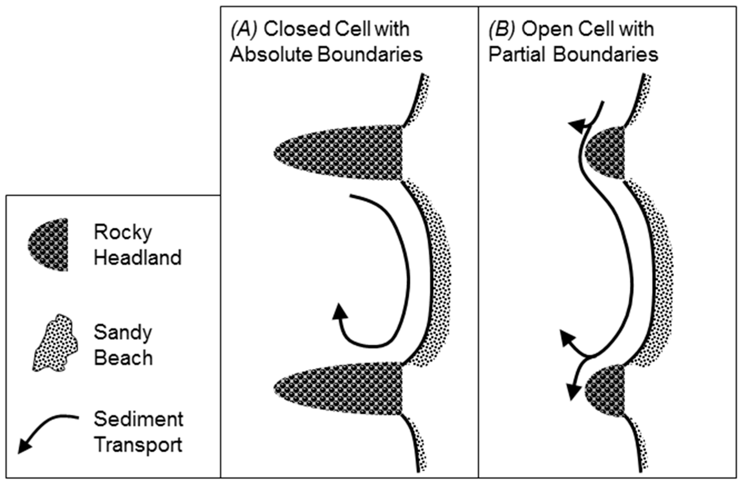
Figure 2.
Size and sharpness of the eight headland classes developed by George, Largier, Storlazzi, and Barnard [27]. Four idealized headlands were developed for modeling using the dimensions of T1, T6, T7, and T8. For examples of the classes, see George, Largier, Storlazzi and Barnard [27].

Figure 3.
Grids, bathymetry, and cross-shore profiles used in modeling study. (A) Computational grids for SWAN1 (blue), FLOW (black), and SWAN2 (red). Bathymetry and plan view of headlands shown with the headland noted by black line, 2.5-km long cross-shore transects at the headland shoulders as dashed lines, and contours at 10-m intervals for T1 (B), T6 (C), T7 (E), and T8 (F). (D) Cross-shore profiles at the apex of the headlands showing the protrusion into the flow field compared to the base line located away from the headland.
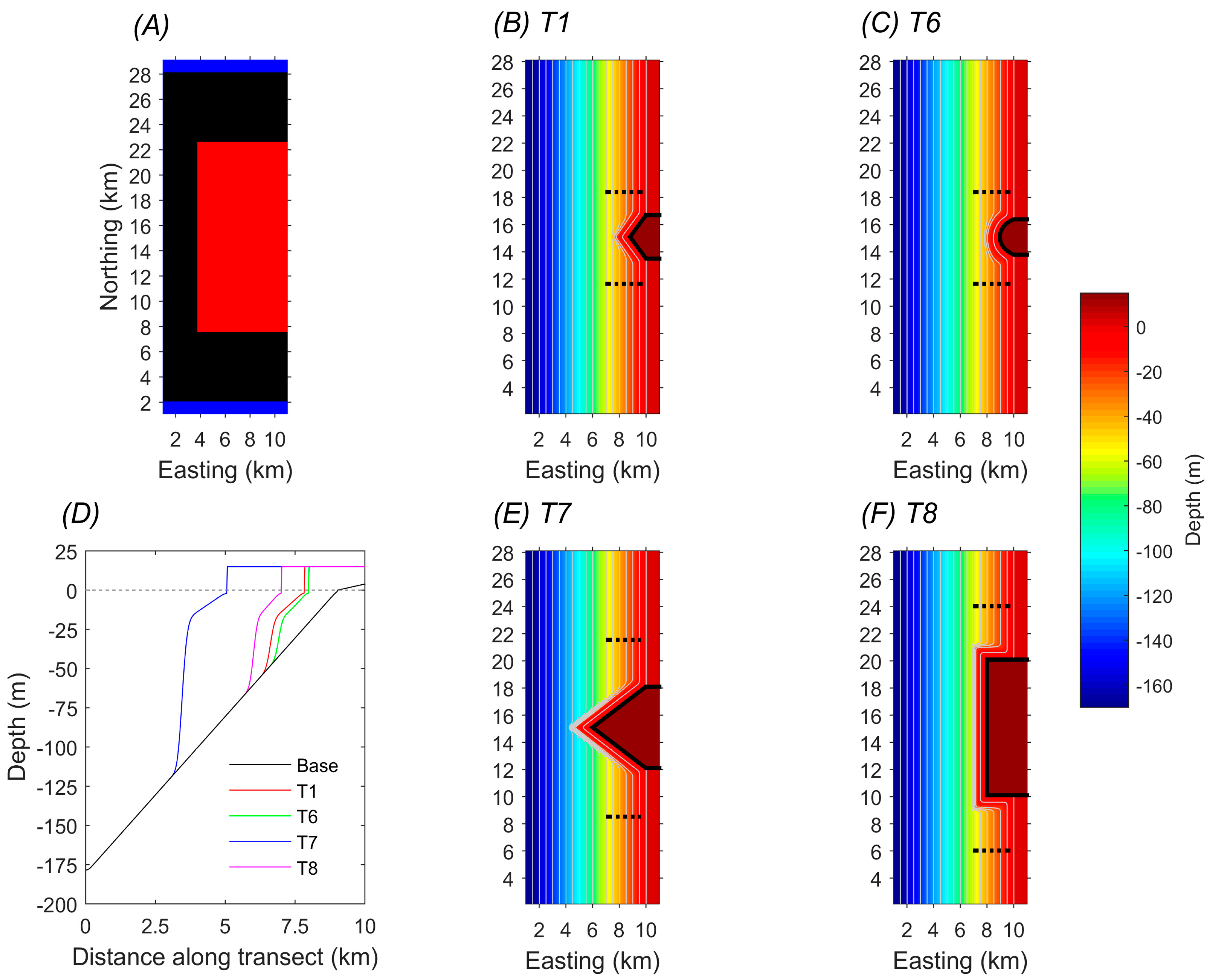
Figure 4.
Schematic depicting categories of βheadland as defined in Equation (13).

Figure 5.
Model results of current speed for waves only and for waves with a regional current forcing during the fastest velocity timestep where L = least wave power, M = most wave power, D = direct wave angle, O = oblique wave angle, and C = regional current. Row A is Headland T1, Row B is T6, Row C is T7, and Row D is T8.

Figure 6.
Cumulative total transport of the three grain sizes through a 2.5-km wide cross-shore transect on the northern and southern headland shoulders and across the headland apex. Results from the baseline simulation were excluded, as sediment transport volumes were negligible. Positive values indicate northward (upstream) transport; negative values indicate southward (downstream) transport.

Figure 7.
Sediment bypassing ratios between northern and southern shoulders for (A) fine (125 μm), (B) fine–medium (250 μm), and (C) medium (500 μm) sand under variable forcing conditions and substrates (Table 2). Baseline calculations were excluded as sediment transport volumes were negligible. The dashed line indicates βheadland = 0.5 as a division inside the “constrained” zone. See Equation (13) for definitions of βheadland categories.

Figure 8.
(a) Model observations from an alongshore transect 400 m offshore from 25% the length of the headland upstream to downstream during the time-step of fastest velocity. The headland is marked by the gray box and the apex by the dashed line in the center. The dashed lines in panel D indicate 45° and −45°. Parameters shown are (A) water level, (B) current speed and direction, (C) wave power and wave direction, (D) current and wave angle relative to the shoreline, (E) total bed shear stress from combined waves and currents and radiation stress from waves, (F) total sediment flux for fine (blue), fine–medium (green), and medium (red) sand, and (G) total sediment deposition (same colors) for T1. (b) Same as (a) for T6. (c) Same as (a) for T7. (d) Same as (a) for T8 with the shore normal faces of the headland noted as the lighter gray boxes.
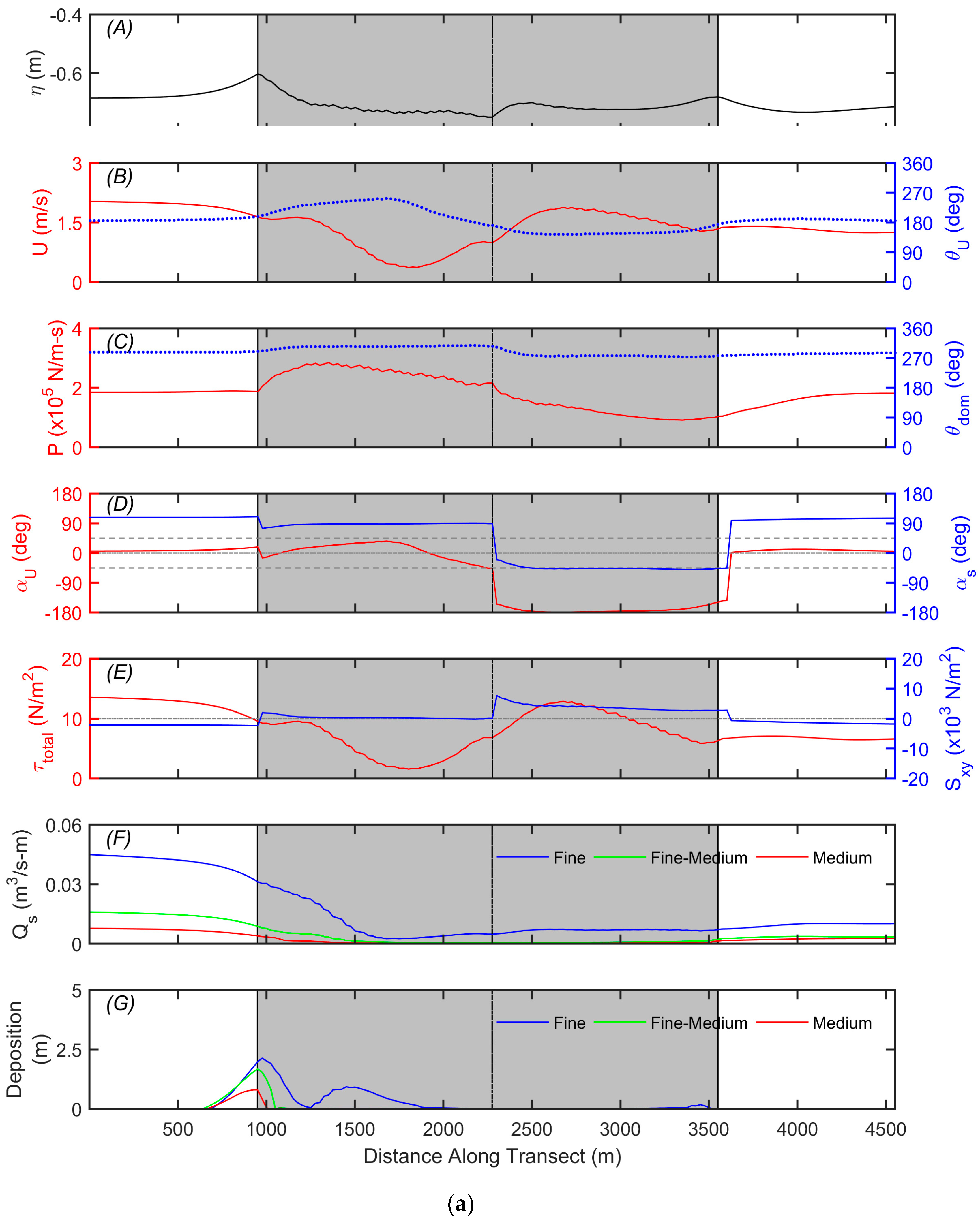

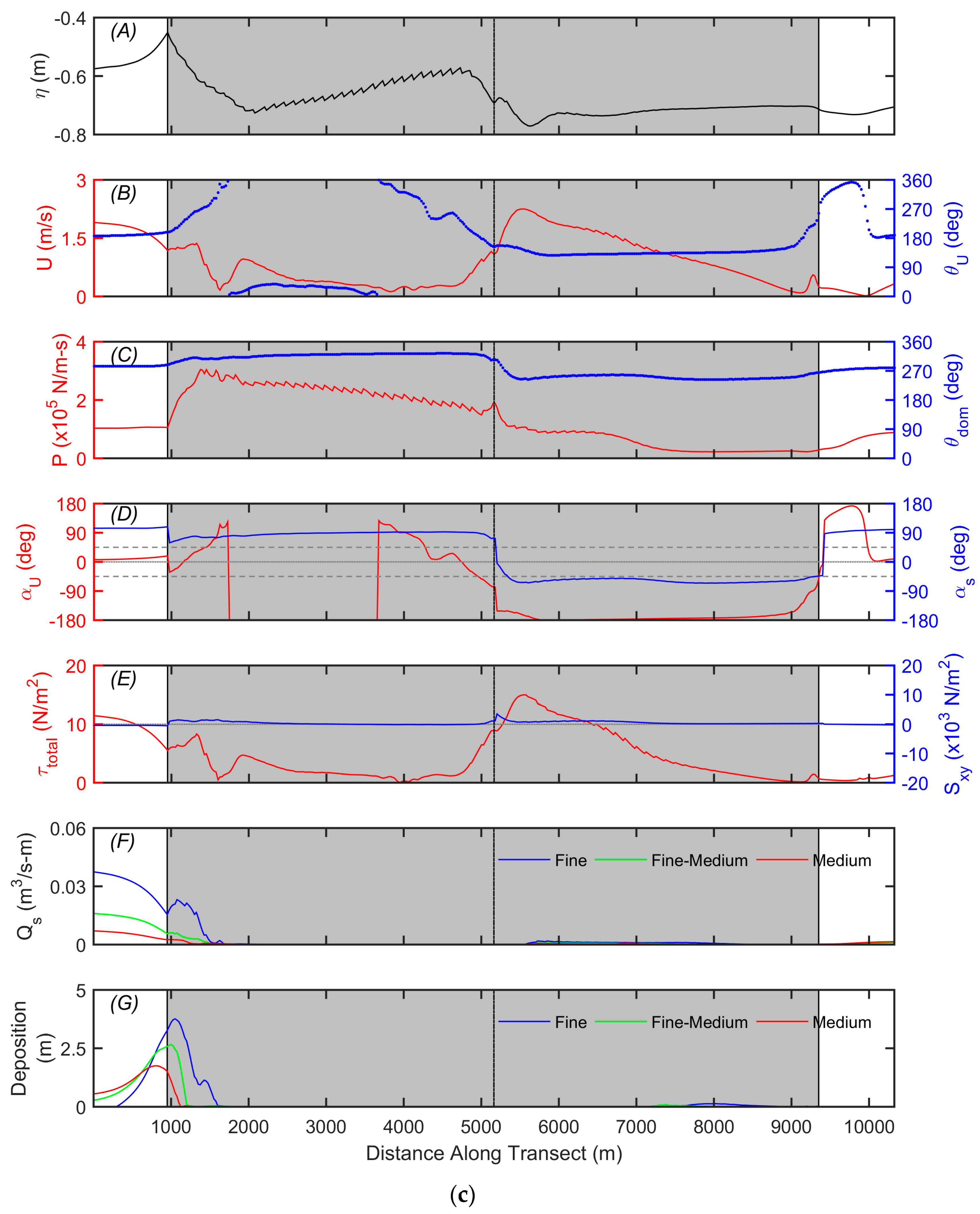
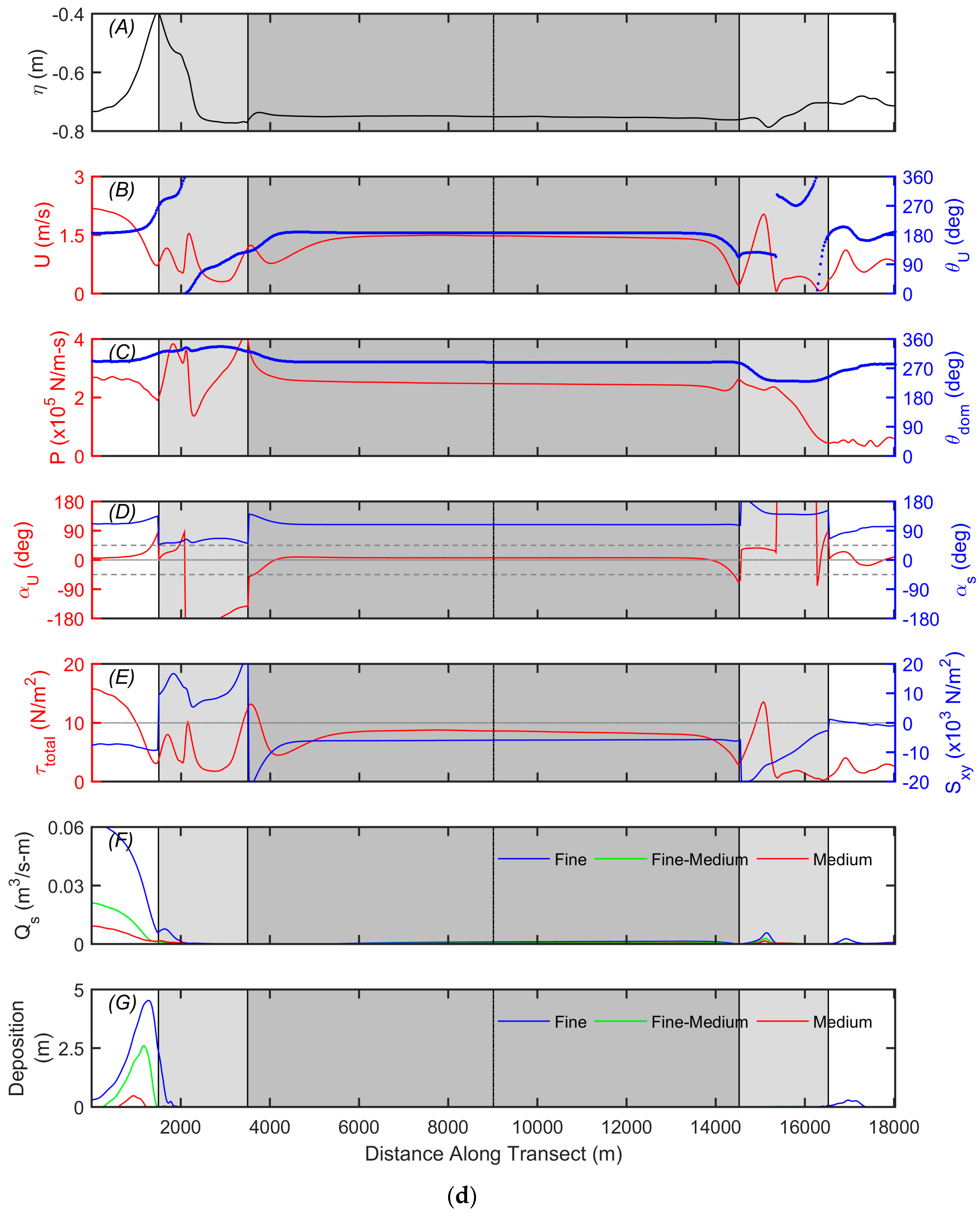
Figure 9.
Summary of sediment bypassing a headland based on βheadland for all grain sizes. See Equation (13) for definitions of βheadland categories.
Figure 9.
Summary of sediment bypassing a headland based on βheadland for all grain sizes. See Equation (13) for definitions of βheadland categories.

Figure 10.
Conceptual sediment pathways and deposition zones for fine and coarse sediment under direct (A, C, E, G) and oblique (B, D, F, H) wave angles for the four generalized headlands.
Figure 10.
Conceptual sediment pathways and deposition zones for fine and coarse sediment under direct (A, C, E, G) and oblique (B, D, F, H) wave angles for the four generalized headlands.
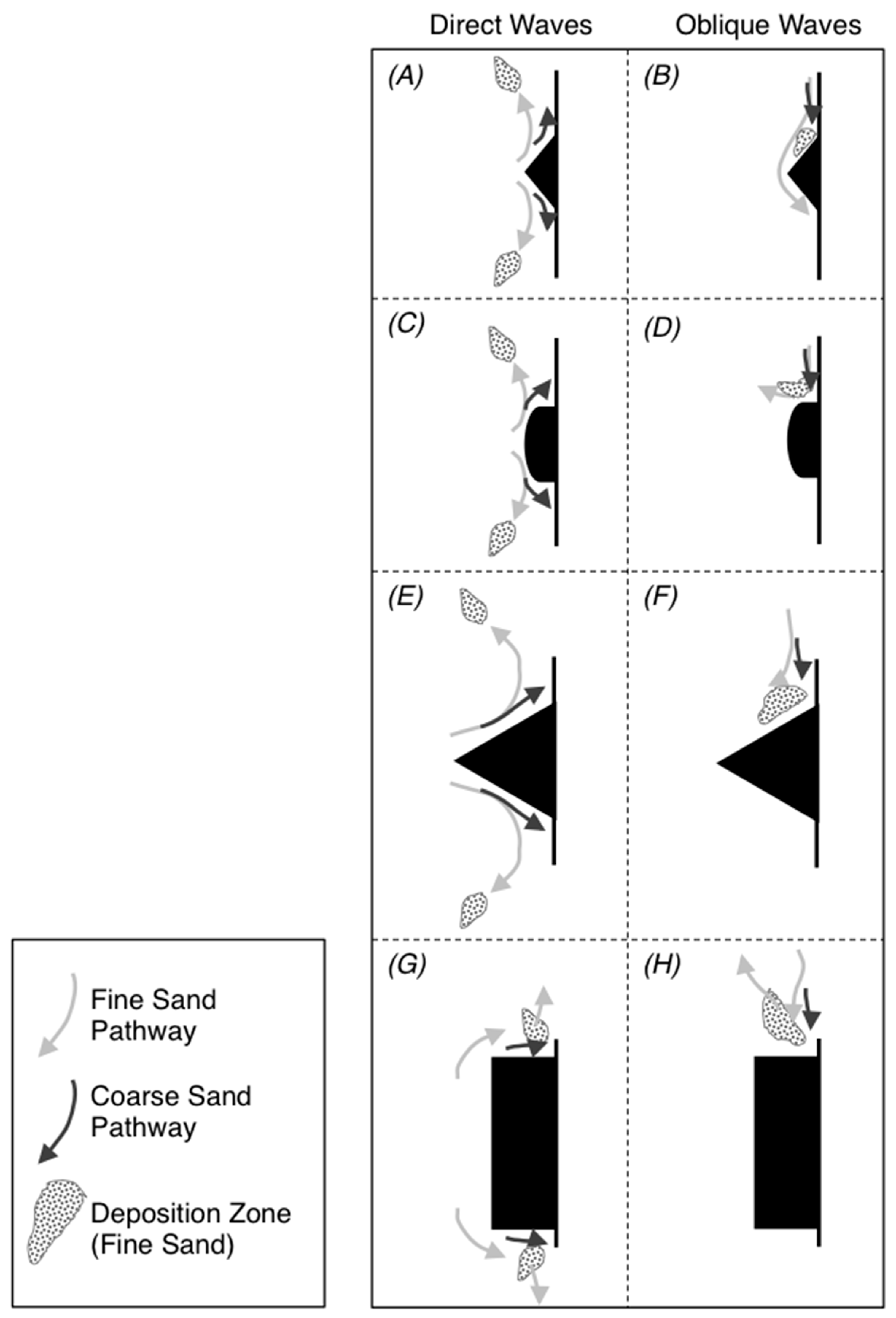

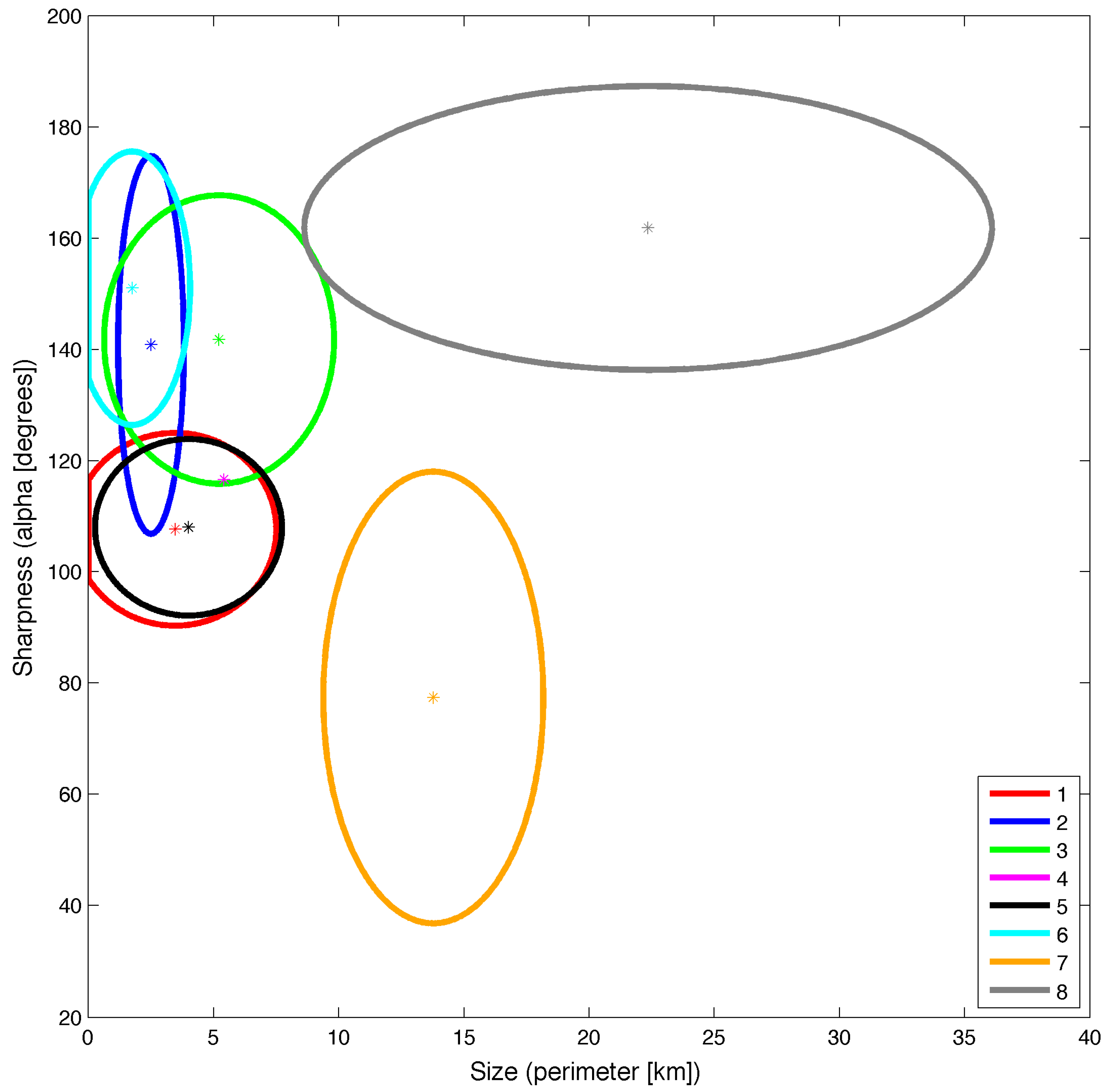
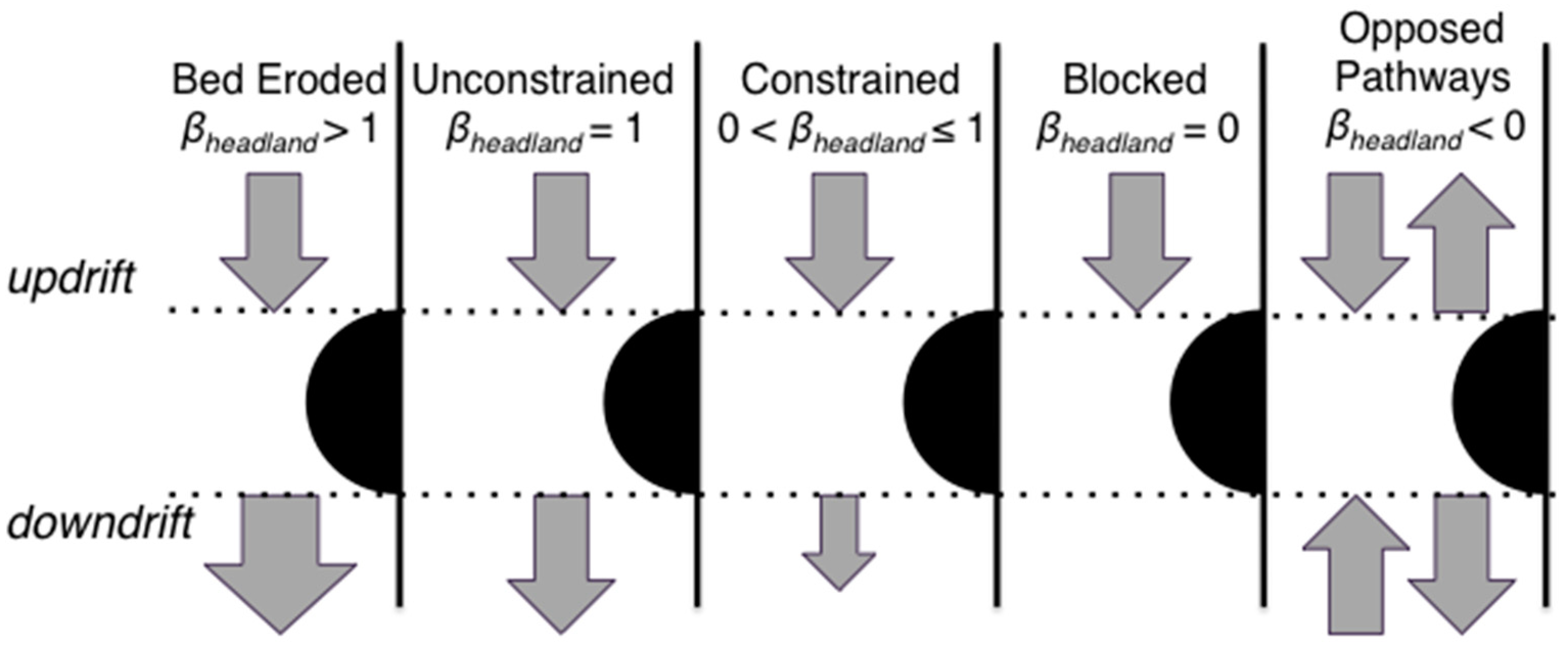
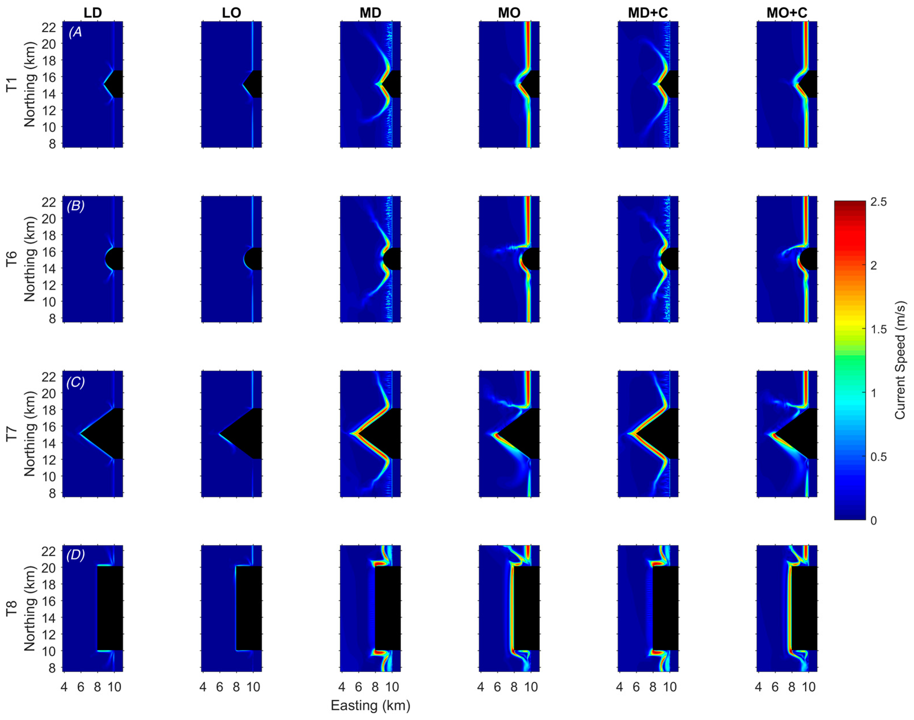
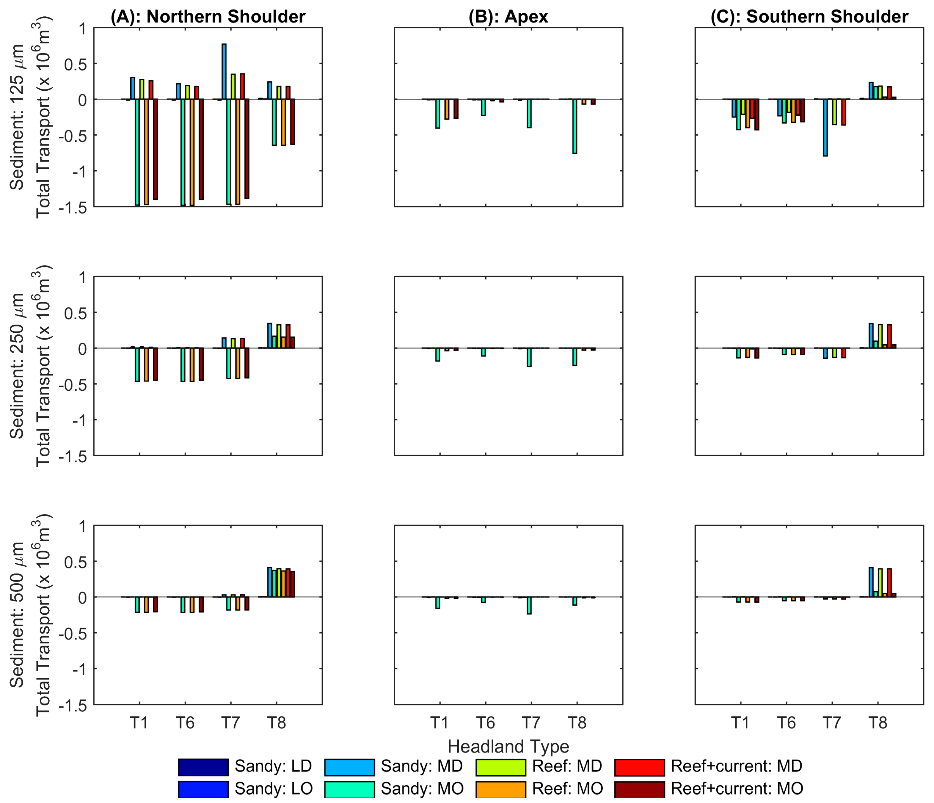
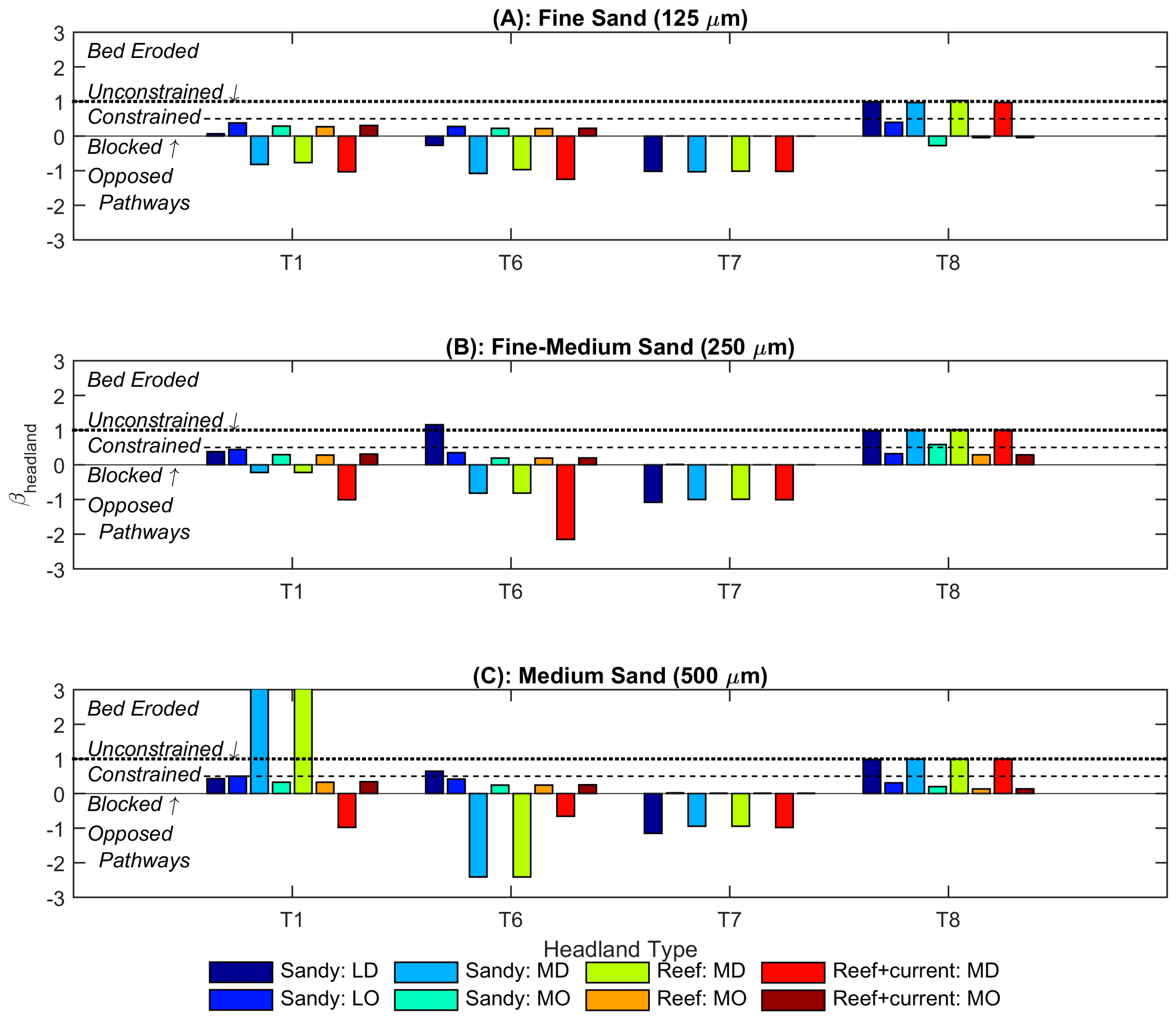
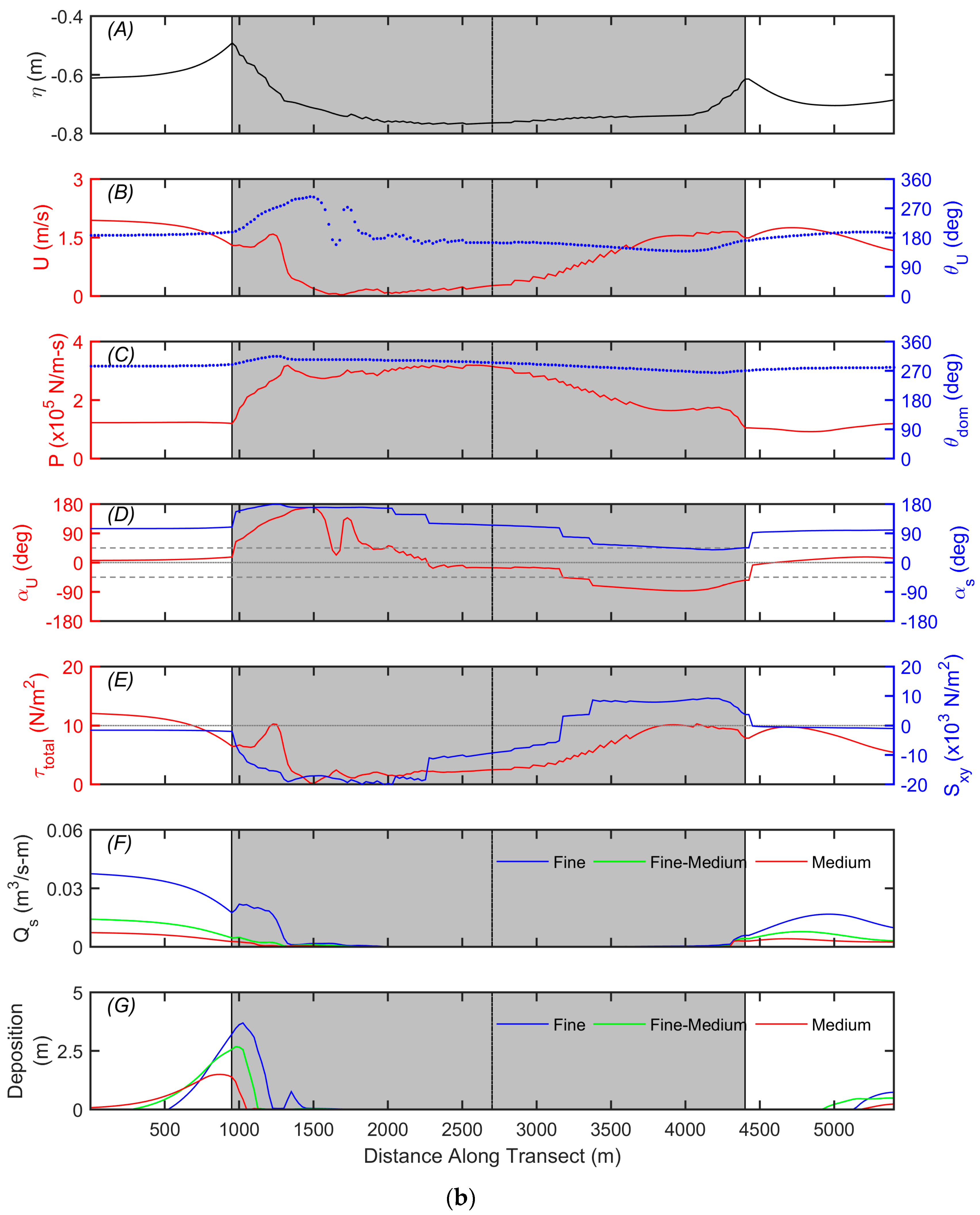
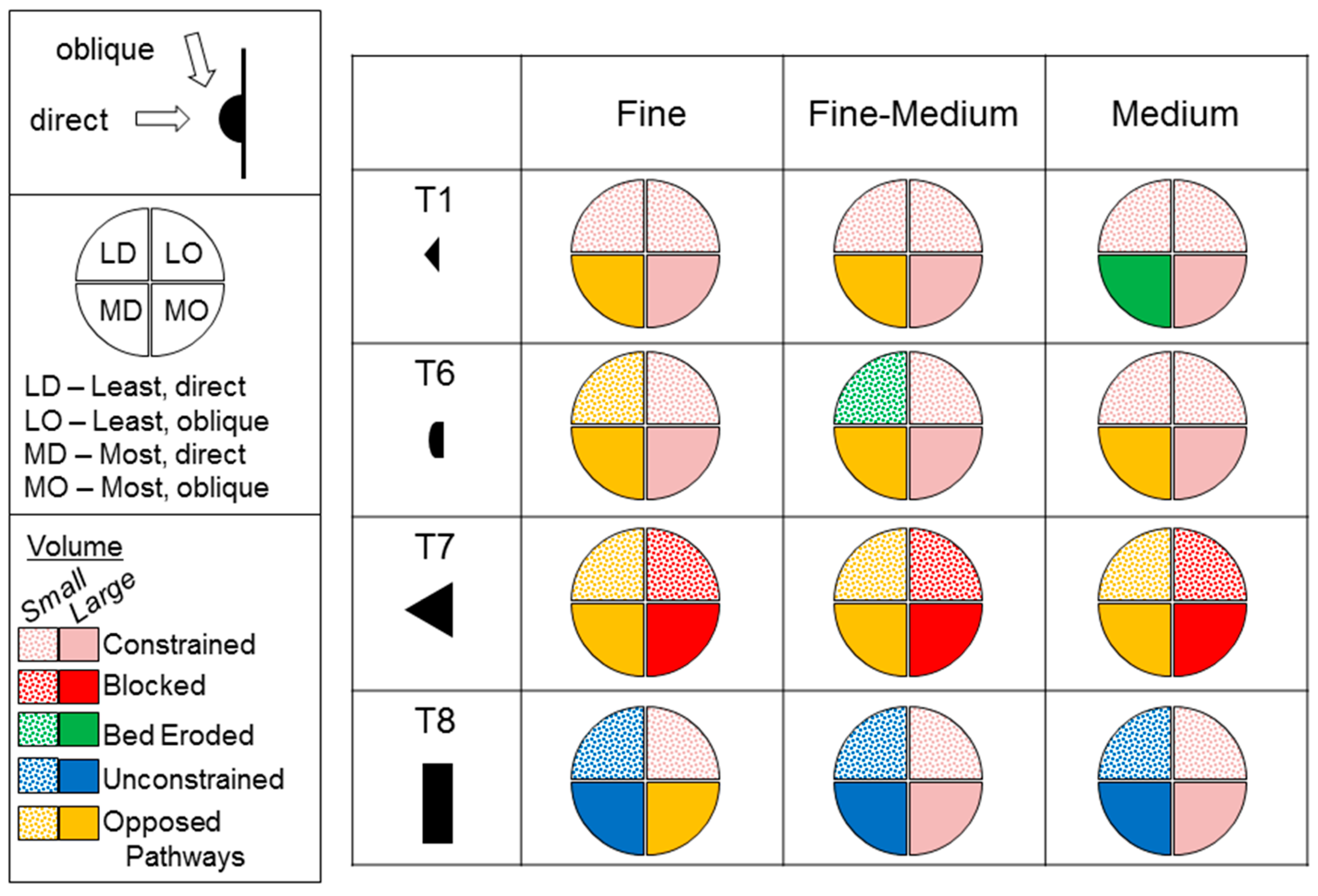
Table 1.
Factors influencing sediment bypassing a headland.
| Factor | Parameter 1 | Spectrum | ||
|---|---|---|---|---|
| Morphology | Headland Size | Small 3 | Medium 3 | Large 3 |
| Headland Shape | Pointed 3 | Curved | Blocky 3 | |
| Headland Symmetry | Upstream Skew | Balanced 3 | Downstream Skew | |
| Aspect Ratio | Length >> Width | Length = Width | Length << Width | |
| Nearshore Shelf Width | Narrow | Medium 3 | Wide | |
| Adjacent Slope | Upstream Deeper | Balanced 3 | Downstream Deeper | |
| Headland-Beach Intersection | Acute | Right | Oblique | |
| Shoreline Rugosity | Smooth 3 | Mixed | Rugged | |
| Offshore of Apex | Ocean 3 | Submerged Reef | Island | |
| Forcing Terms | Wave Height | Small 3 | Medium | Large 3 |
| Wave Period | Short 3 | Medium | Long 3 | |
| Deep Water Wave Angle | Direct (e.g., 270) 3 | Middle (e.g., 315) | Oblique (e.g., 345) 3 | |
| Tidal Range | Micromareal | Mesomareal 3 | Macromareal | |
| Regional Current Speed | None 3 | Slow 3 | Fast | |
| Regional Current Direction | Heading 3 | Across | Following | |
| Wind Speed | None | Slow 3 | Fast | |
| Wind Direction | Onshore | Alongshore 3 | Offshore | |
| Coriolis | Equator | Mid-latitudes 3 | Pole | |
| Sediment | Sediment Type | Muds | Sands 3 | Pebbles |
| Sediment Size (e.g., sand) | Fine 3 | Fine–Medium 3 | Medium 3 | |
| Substrate | Sandy 3 | Mixed | Reef 3 | |
| Sediment Source 2 | Fluvial | Cliff Erosion | Marine 3 | |
1 Bold-face indicates a parameter tested in the current study; 2 “Spectrum” does not apply to describe range of sediment sources; 3 Variability of parameters in current study where applicable; aspect ratio and headland–beach intersection dependent on headland size and shape.
Table 2.
Numerical model simulations for each headland type and grain size.
| Simulation | Hydrodynamics | Substrate | |||||||||
|---|---|---|---|---|---|---|---|---|---|---|---|
| Description | Tides | Waves | Currents | Sandy | Reef | ||||||
| LD | LO | MD | MO | ||||||||
| Baseline | X | - | - | - | - | - | X | - | |||
| Sandy Bed | X | X | X | X | X | - | X | - | |||
| Reefed Headland | X | - | X | X | X | - | - | X | |||
| Regional Current | X | - | - | X | X | X | - | X | |||
L = Least Wave Power, M = Most Wave Power, D = Direct Wave Angle, O = Oblique Wave Angle.
Table 3.
Design of idealized headlands based on George, Largier, Storlazzi, and Barnard [27] (G2015) Classification.
Table 3.
Design of idealized headlands based on George, Largier, Storlazzi, and Barnard [27] (G2015) Classification.
| Headland Class | Description (Size, Apex) | Occurrence of Class in G2015 | Alongshore Length (m) 1 | Cross-shore Distance (m) 1,2 | Apex Angle (deg) |
|---|---|---|---|---|---|
| T1 | Small, medium | 28% | 3200 | 1200 | 107° |
| T6 | Small, broad | 26% | 2600 | 1100 | 151° |
| T7 | Medium, sharp | 6% | 6200 | 2900 | 77° |
| T8 | Large, broad | 6% | 10,000 | 2,000 | 180° |
1 For headland only, not adjacent to surfzone; 2 Measured from beach–headland intersection point.
Table 4.
Major tidal constituents at Port San Luis, California and calculated C1.
| Constituent | Amplitude (m) | Phase (deg) |
|---|---|---|
| M2 | 0.50 | 296° |
| S2 | 0.15 | 30° |
| N2 | 0.12 | 28° |
| K1 | 0.36 | 15° |
| O1 | 0.23 | 14° |
| C1 * | 0.41 | 91° |
* See Equations (1) and (2).
Table 5.
Wave conditions for forcing numerical models.
| Incident Wave Angle | Wave Power Parameters | |
|---|---|---|
| Least | Most | |
| Direct | Hs = 2 m | Hs = 7 m |
| Tp = 10 s | Tp = 16 s | |
| θdom = 270° | θdom = 270° | |
| Oblique | Hs = 2 m | Hs = 7 m |
| Tp = 10 s | Tp = 16 s | |
| θdom = 345° | θdom = 345° | |
Table 6.
Ratios for Mfactor1 (see Equation (3)) with oblique wave angles.
| Least Wave Power | |||||
|---|---|---|---|---|---|
| T1 | T6 | T7 | T8 | ||
| Most Wave Power | T1 | - | 2.50 | 0.57 | 0.96 |
| T6 | 1.08 | - | 0.23 | 0.38 | |
| T7 | 1.20 | 1.11 | - | 1.68 | |
| T8 | 0.75 | 0.69 | 0.62 | - | |
Table 7.
Ratios for (a) Mfactor2 and (b) Mfactor3.
| (a) see Equation (4) | Volume Deposited | ||||
|---|---|---|---|---|---|
| Fine Sand | T1 | T6 | T7 | T8 | |
| T1 | - | - | - | - | |
| T6 | 1.13 | - | - | - | |
| T7 | 0.73 | 0.65 | - | - | |
| T8 | 0.49 | 0.44 | 0.68 | - | |
| Fine–Medium Sand | T1 | T6 | T7 | T8 | |
| T1 | - | - | - | - | |
| T6 | 1.31 | - | - | - | |
| T7 | 0.72 | 0.55 | - | - | |
| T8 | 0.56 | 0.43 | 0.78 | - | |
| Medium Sand | T1 | T6 | T7 | T8 | |
| T1 | - | - | - | - | |
| T6 | 1.41 | - | - | - | |
| T7 | 0.69 | 0.49 | - | - | |
| T8 | 0.58 | 0.41 | 0.83 | - | |
| (b) see Equation (5) | Area of Deposition | ||||
|---|---|---|---|---|---|
| Fine Sand | T1 | T6 | T7 | T8 | |
| T1 | - | - | - | - | |
| T6 | 1.44 | - | - | - | |
| T7 | 0.87 | 0.60 | - | - | |
| T8 | 0.58 | 0.40 | 0.66 | ||
| Fine–Medium Sand | T1 | T6 | T7 | T8 | |
| T1 | - | - | - | - | |
| T6 | 1.12 | - | - | - | |
| T7 | 0.57 | 0.51 | - | - | |
| T8 | 0.36 | 0.33 | 0.64 | - | |
| Medium Sand | T1 | T6 | T7 | T8 | |
| T1 | - | - | - | - | |
| T6 | 1.39 | - | - | - | |
| T7 | 0.63 | 0.45 | - | - | |
| T8 | 0.40 | 0.28 | 0.62 | - | |
Table 8.
Ratios for all Ofactors.
| Ofactor1 | Ofactor2 | Ofactor3 | ||
|---|---|---|---|---|
| See: | (6) | (7) | (8) | |
| Fine Sand | T1 | 0.06 | 0.02 | 0.90 |
| T6 | 0.01 | 0.01 | 0.94 | |
| T7 | 0.00 | 0.01 | 0.94 | |
| T8 | 0.54 | 0.00 | 0.97 | |
| Fine-Medium Sand | T1 | 0.04 | 0.02 | 0.93 |
| T6 | 0.00 | 0.02 | 0.96 | |
| T7 | 0.00 | 0.01 | 0.98 | |
| T8 | 5.98 | 0.01 | 1.00 | |
| Medium Sand | T1 | 0.03 | 0.03 | 0.94 |
| T6 | 0.00 | 0.03 | 0.96 | |
| T7 | 0.01 | 0.02 | 0.99 | |
| T8 | 2.50 | 0.00 | 0.98 |
Table 9.
Ratios for (a) Sfactor1 and Sfactor2 and (b) Sfactor3 and Sfactor4.
| (a) | Grain Size Comparison | |||
|---|---|---|---|---|
| Sfactor1 | Sfactor2 | |||
| See: | (9)a | (9)b | (10)a | (10)b |
| T1 | 1.73 | 0.84 | 3.37 | 0.82 |
| T6 | 2.01 | 0.78 | 2.61 | 0.65 |
| T7 | 1.70 | 0.87 | 2.21 | 0.73 |
| T8 | 1.96 | 0.81 | 2.12 | 0.75 |
| Mean | 1.85 ± 0.16 | 0.82 ± 0.04 | 2.58 ± 0.57 | 0.74 ± 0.07 |
| (b) | Substrate Comparison | ||
|---|---|---|---|
| Sfactor3 | Sfactor4 | ||
| See: | (11) | (12) | |
| Fine Sand | T1 | 1.44 | 1.27 |
| T6 | 1.62 | 1.42 | |
| T7 | 1.25 | 1.32 | |
| T8 | 2.24 | 1.61 | |
| Mean | 1.64 ± 0.43 | 1.41 ± 0.15 | |
| Fine–Medium Sand | T1 | 1.80 | 2.24 |
| T6 | 2.21 | 2.27 | |
| T7 | 1.32 | 1.57 | |
| T8 | 2.78 | 1.84 | |
| Mean | 2.03 ± 0.62 | 1.98 ± 0.34 | |
| Medium Sand | T1 | 2.02 | 2.56 |
| T6 | 2.51 | 3.04 | |
| T7 | 1.53 | 1.90 | |
| T8 | 2.86 | 1.88 | |
| Mean | 2.23 ± 0.58 | 2.34 ± 0.56 | |
Table 10.
Alongshore transect results for forcings and sediment response.
| Transect length (m) | Δη (m) | U (m/s) | θU (deg) | P (×105 N/m-s) | θdom (deg) | αU (deg) | αs (deg) | ||||||||
|---|---|---|---|---|---|---|---|---|---|---|---|---|---|---|---|
| N * | S * | N | S | N | S | N | S | N | S | N | S | N | S | ||
| T1 | 4500 | 0.15 | 0.07 | 0.4–2.0 | 1.0–1.8 | 186-–250 | 144–190 | 1.9–2.8 | 0.9–1.8 | 287–307 | 276–306 | −45–36 | −174–10 | 78–108 | −49–99 |
| T6 | 5500 | 0.27 | 0.15 | <0.1–2.0 | 0.3–1.8 | 186–305 | 138–197 | 1.2–3.1 | 0.9–3.1 | 285–314 | 264–292 | −15–170 | −89–17 | 104–180 | 39–115 |
| T7 | 10,000 | 0.27 | 0.10 | 0.1–2.0 | <0.1–2.3 | 0–360 | 126–353 | 1.0–3.0 | 0.2–1.9 | 284–324 | 244–305 | 7–123/180 | −180–173 | 76–104 | −62–95 |
| T8 | 18,000 | 0.36 | 0.11 | 0.3–2.1 | <0.1–2.0 | 0–360 | 0–360 | 1.3–4.0 | 0.3–2.6 | 291–336 | 230–288 | −180–83 | −67–180 | 47–135 | 65–180 |
| τtotal (N/m2) | Sxy (×103 N/m2) | Qs max (fine) (m3/s-m) | Qs max (f-m) (m3/s-m) | Qs max (med) (m3/s-m) | Deposition max (fine) (m) | Deposition max (f-m) (m) | Deposition max (med) (m) | |||||||||
|---|---|---|---|---|---|---|---|---|---|---|---|---|---|---|---|---|
| N | S | N | S | N | S | N | S | N | S | N | S | N | S | N | S | |
| T1 | 1.5–13.5 | 5.8–12.9 | −2–1.9 | −1.5–7 | 0.04 | 0.01 | 0.02 | <0.01 | 0.01 | <0.01 | 2.1 | 0.2 | 1.7 | 0 | 0.8 | 0 |
| T6 | 0.2–12 | 2.4–9.7 | −1.6–−2.0 | −9.1–9.1 | 0.04 | 0.02 | 0.01 | 0.01 | <0.01 | <0.01 | 3.7 | 0.7 | 2.7 | 0.4 | 1.5 | 0.2 |
| T7 | 0.2–11.4 | 0.2–15 | −0.4–1.1 | 0–3.0 | 0.04 | <0.01 | 0.01 | <0.01 | <0.01 | <0.01 | 3.7 | 0.1 | 2.6 | 0 | 1.7 | 0 |
| T8 | 1.7–15 | 0.6–12.4 | −20–20 | −20–1.2 | 0.06 | 0 | 0.02 | 0 | <0.01 | <0.01 | 4.5 | 0.3 | 2.6 | 0 | 0.5 | 0 |
* N: Northern (or updrift) and * S: Southern (or downdrift) faces of headland as determined by the headland apex.
Table 11.
Incident waves on northern faces of headlands by wave angle.
| Headland Class | Headland Shoreline Angle (from North) | Direct Wave (270°) | Oblique Wave (345°) | ||
|---|---|---|---|---|---|
| αb | sin(2αb) * | αb | sin(2αb) * | ||
| T1 | 217° | 53° | 0.96 | 128° | −0.97 |
| T6 | 195° | 75° | 0.50 | 150° | −0.87 |
| T7 | 231° | 39° | 0.98 | 114° | −0.74 |
| T8 | 90° (north) | 180° | 0.00 | 255° | 0.50 |
| 180° (west) | 90° | 0.00 | 165° | −0.50 | |
* Scales Pab in Equation (16) as 0 = no transport, ±1 = maximum transport.
© 2019 by the authors. Licensee MDPI, Basel, Switzerland. This article is an open access article distributed under the terms and conditions of the Creative Commons Attribution (CC BY) license (http://creativecommons.org/licenses/by/4.0/).
Share and Cite
MDPI and ACS Style
George, D.A.; Largier, J.L.; Pasternack, G.B.; Barnard, P.L.; Storlazzi, C.D.; Erikson, L.H. Modeling Sediment Bypassing around Idealized Rocky Headlands. J. Mar. Sci. Eng. 2019, 7, 40. https://doi.org/10.3390/jmse7020040
AMA Style
George DA, Largier JL, Pasternack GB, Barnard PL, Storlazzi CD, Erikson LH. Modeling Sediment Bypassing around Idealized Rocky Headlands. Journal of Marine Science and Engineering. 2019; 7(2):40. https://doi.org/10.3390/jmse7020040
Chicago/Turabian StyleGeorge, Douglas A., John L. Largier, Gregory Brian Pasternack, Patrick L. Barnard, Curt D. Storlazzi, and Li H. Erikson. 2019. "Modeling Sediment Bypassing around Idealized Rocky Headlands" Journal of Marine Science and Engineering 7, no. 2: 40. https://doi.org/10.3390/jmse7020040
Note that from the first issue of 2016, this journal uses article numbers instead of page numbers. See further details here.