An Approach for Predicting the Specific Fuel Consumption of Dual-Fuel Two-Stroke Marine Engines

Abstract

Increasing environmental demands, alongside the planned penetration of natural gas as marine fuel, have rendered dual-fuel engines as an attractive prime mover alternative. In this context, knowing the specific fuel consumption is essential to selecting the most efficient engine. The specific fuel consumption can be approached by simulation models with varying levels of complexity that are either implemented by basic programming languages or simulated by dedicated packages. This study aims to develop a simplified model to predict the specific fuel consumption of dual-fuel two-stroke marine engines driving fixed or controllable pitch propellers. The model relies on clear trends approachable by polynomials that were revealed by normalizing specific fuel consumption. This model requires only the value of specific fuel consumption at a nominal maximum continuous rating to predict the engine consumption at any specified rating, including at partial engine load. The outcome of the study shows that the maximum deviations regarding the two simulated engines did not exceed −3.6%. In summary, the proposed model is a fast and effective tool for optimizing the selection of dual-fuel, two-stroke Diesel engines regarding fuel consumption.

1. Introduction

The maritime industry has faced new realities that have been changing marine fuel investment choices over the last few decades. Although vessels have become cleaner, regulators, environmentalists, and health officials have still been concerned about pollutants near major coastal population centres [1]. Furthermore, the decision to implement a global sulphur cap of 0.5% in 2020, revising the current 3.5% cap (outside sulphur emission control areas), was presented in the Resolution MEPC.176(58) [2] and confirmed by the International Maritime Organisation (IMO) on October 2016 [3]. This change applies globally and will affect as many as 70,000 ships, which is a reason why experts do not agree completely with the IMO’s study that indicates the refineries will be capable of providing the required amount of low-sulphur marine fuel by 2020 [4].

Natural gas offers lower local pollution emissions compared to distillate fuels, and can significantly reduce local pollutants from vessel operations. Price differences between natural gas and low-sulphur fuel oil suggest that an economic advantage may favor the use of natural gas. In addition, natural gas infrastructure has been growing, rendering ships fed by natural gas more plausible [1]. These have been some of the reasons why dual-fuel Diesel engines have become an attractive prime mover alternative.

The term “dual-fuel” describes compression ignition engines burning two different fuels simultaneously in varying proportions. In gas mode, gaseous fuel supplies most of the energy released through combustion, whereas liquid fuel is employed to provide the energy needed for ignition [5]. Hence, in this operation mode, there are two specific fuel consumptions: specific gas consumption (SGC), and specific pilot oil consumption (SPOC). In Diesel mode, these engines work as a conventional Diesel engine, such that there is only specific fuel oil consumption (SFOC).

Knowing these parameters is essential for selecting the most efficient engine and estimating its gaseous emission. The fuel consumption is the primary driver for operational expenditures, and it is directly linked to carbon dioxide emission, which is one of the greenhouse gases. Thus, in an optimization study, it is sought to select the engine of the least specific fuel consumption. Moreover, predicting the amount of fuel to be consumed in a journey is essential to design the fuel supply system. These are some of the reasons why the prediction of specific fuel consumption is relevant and addressed herein.

Internal combustion engine simulation consists in reproducing mathematically the significant processes, and predicting performance and operating details. The mathematical formulation for this purpose may be implemented through many scientific languages, such as Fortran, MatLab, GNU Octave, Scilab, C#, and C++. Some simulation-dedicated packages may also be applied, such as CORAL, CSMP, ACSL, Xcos, and SIMULINK. Furthermore, dedicated software, such as AVL BOOST, GT-POWER, and VIRTUAL ENGINE, may be applied for engine 0-D simulations, whilst multi-dimensional simulations may be performed through CONVERGE, KIVA, FLUENT, CFX, OpenFOAM, ANSYS Forte, and others [6].

The five main sorts of engine models in descending order of complexity are: computational fluid dynamics (CFD) models, phenomenological multi-dimensional models, crank angle models, mean value models, and transfer function models [7]. In CFD modelling, the volume studied is divided into thousands of parts, and the basic conservation equations are solved for every single part. This provides detailed information and requires powerful computers and high computational time. On the other hand, if the cylinder is divided into tens of volumes and phenomenological equations are included, a phenomenological multi-dimensional model is obtained. Crank angle models are also called zero-dimensional (0-D) because they do not have a strict mathematical dependence on any of the dimensions. It treats each of the various engine elements as a control volume and solves the differential equations in a time-step equivalent to one degree of the crankshaft rotation. Nevertheless, once the engine model is inserted into a larger system, such as a propulsion system, the variations occurring at each crankshaft angle are generally not important. In such cases, overall engine operating parameters are the focus, and they can be obtained by using a mean-value engine model (MVEM). This model has basically the same origin as the 0-D, but as its time-step is in the order of one crankshaft rotation, the variation of each parameter in the cylinder is replaced by a mean value. Finally, once there is no interest at all in the internal processes, the engine can be merely represented by functions. This is the so-called transfer function engine model (TFEM), which is the fastest method.

As the development of marine Diesel engines is a time-consuming and costly procedure, detailed engine-modelling techniques have been used for investigating the engine’s steady-state performance and transient response, as well as for testing the alternative designs of the engine systems. Performance under fault conditions [8], the formation of noxious emissions [9,10,11], the employment of exhaust gas recirculation to decrease it [12], and instantaneous change in the properties of exhaust gas [13] besides the condensation of combustion products [14] may be assessed by 0-D modelling. On the other hand, the simulation of in-cylinder flow on different piston-bowl geometries [15], the investigation of soot formation and oxidation processes [16], as well as the investigation of the effects of inlet pressure, exhaust-gas recirculation, and the start of injection time on gaseous emissions [17], may be performed by CFD modelling.

In certain types of systems, a large number of components and feasible alternatives regarding design specifications and operating conditions makes the use of simulation and optimization techniques rather imperative to find a technical and economical attractive solution. In this context, dynamic simulations of the propulsion plant were explored in [18,19,20,21] whilst the synthesis, design, and/or operation optimization was addressed in [22,23,24,25,26]. In the majority of the works, the engine was modelled by means of the TFEM [18,21,23,24,25,26,27] and the MVEM was employed in a few of them [19,20]. This is due to the ease and speed of those models, as well as to the usual disinterest in in-cylinder parameters for engines inserted in larger systems. The simplest approach considered the prime mover as a constant value of specific fuel consumption [22]. Two-stroke Diesel engines were employed in [19,20,23] whilst a dual-fuel two-stroke Diesel engine was used in only one study [26].

In reference [26], specific fuel consumptions (SFOC, SPOC, and SGC) were modelled as functions of the specified maximum continuous rating (SMCR) and engine load, which is a fraction of the SMCR. The analysis was conducted by applying polynomial regression and the least square fitting method on data identified in the Project Guide of the engine’s manufacturer [28]. However, specific fuel consumptions for the same SMCR are different to different engines and vary with the engine load for fixed and controllable pitch propeller drivers. Whenever an engine is driving a fixed pitch propeller, the Project Guide considers brake power and speed linked by the propeller law [29], whilst for controllable pitch propeller, speed is considered constant. Since these aspects were not considered, the main contribution of the present work is the development of an engine model suitable to optimize the selection of dual-fuel two-stroke Diesel engines considering the uniqueness of each engine and the propeller type to be driven.

2. Methodology

The algorithms included in the proposed model were implemented in a MatLab environment. Including engine data from various manufacturers would be ideal in this sort of study, but the required information is not readily provided by the most engine manufacturers. Therefore, owing to the broad data availability of a web-based application from a two-stroke Diesel engine manufacturer [28], only Diesel engines covered by this application were studied. Standard ambient conditions provided by the International Organization for Standardization and a sulphur content of 0.5% were assumed. Although engine type designation refers to the number of cylinders, stroke/bore ratio, diameter of piston, engine concept, mark number, fuel injection concept, and Tier III technology, narrow configurations of engines were studied. All the addressed engines were not equipped with Tier III technology, and they held the same fuel injection concept (GI) and engine concept (ME-C). Furthermore, only default configurations of engines were taken into account.

Two-stroke marine engine selection begins with placing the SMCR point on the engine layout diagram programme to identify engines able to supply the required power and speed. An engine layout diagram is an envelope that defines the field where nominal maximum firing pressure is available [30]. Every single engine holds a layout diagram depending on its number of cylinders, such that necessary information to plot the layout diagrams for the 22 engines considered herein is presented in

Table 1. Available ME-GI slow-speed dual-fuel engines and their particulars to chart layout diagrams.

Engine	${\mathit{P}}_{\mathit{Bc},\mathit{L}1}$	${\mathit{P}}_{\mathit{Bc},\mathit{L}2}$	${\mathit{P}}_{\mathit{Bc},\mathit{L}3}$	${\mathit{P}}_{\mathit{Bc},\mathit{L}4}$	${\mathit{n}}_{\mathit{min}}$	${\mathit{n}}_{\mathit{max}}$	${\mathit{Z}}_{\mathit{c},\mathit{min}}$	${\mathit{Z}}_{\mathit{c},\mathit{max}}$
	kW/Cylinder				rpm		Cylinder
G95ME-C9.6	6870	5170	6440	4840	75	80	5	12
G95ME-C10.5	6870	5170	6010	4520	70	80	5	12
G95ME-C9.5	6870	5170	6010	4520	70	80	5	12
G90ME-C10.5	6240	4670	5350	4010	72	84	5	12
S90ME-C10.5	6100	4880	5230	4180	72	84	5	12
G80ME-C9.5	4710	3550	3800	2860	58	72	6	9
S80ME-C9.5	4510	3610	4160	3330	72	78	6	9
G70ME-C10.5	3060	2540	2620	2180	66	77	5	6
G70ME-C9.5	3640	2740	2720	2050	62	83	5	8
S70ME-C10.5	3430	2580	2750	2070	73	91	5	8
S70ME-C8.5	3270	2610	2620	2100	73	91	5	8
S65ME-C8.5	2870	2290	2330	1860	77	95	5	8
G60ME-C9.5	2680	2010	1990	1500	72	97	5	8
S60ME-C10.5	2490	1880	2000	1500	84	105	5	8
S60ME-C8.5	2380	1900	1900	1520	84	105	5	8
G50ME-C9.6	1720	1290	1360	1020	79	100	5	9
S50ME-C9.7	1780	1340	1290	970	85	117	5	9
S50ME-C9.6	1780	1420	1350	1080	89	117	5	9
S50ME-C8.5	1660	1330	1340	1070	102	127	5	9
G45ME-C9.5	1390	1045	1090	820	87	111	5	8
G40ME-C9.5	1100	825	870	655	99	125	5	8
S40ME-C9.5	1135	910	865	690	111	146	5	9

. In this table, the brake power per cylinder on the four points of the envelope is listed ($P_{Bc,L1}$, $P_{Bc,L2}$, $P_{Bc,L3}$ and $P_{Bc,L4}$), as well as speed limits ($n_{min}$ and $n_{max}$) and limitations on the number of cylinders ($Z_{c,min}$ and $Z_{c,max}$) for every single engine. As it may be noticed, only engines of type G (green ultra-long stroke) and S (super long stroke), with diameters from 40 to 95 cm and various mark numbers (8.5, 9.5, 9.6...) were studied.

Since specific fuel consumption at SMCR depends on its position on the engine layout diagram, the SMCR was placed on the points L1, L2, L3, and L4, and the specific fuel consumptions of every engine were analyzed. However, specific fuel consumptions at part load depend also on the driven propeller type: fixed pitch propeller (FPP) or controllable pitch propeller (CPP). Hence, the web-based application was run four times for each of the 22 engines, considering FPP and CPP driving, summing up 176 runs. The application provides a table with specific fuel consumption [g/kWh] with loads from 10 to 100% of SMCR. Thus, specific fuel consumptions were normalized and the arising trends were approximated by polynomials.

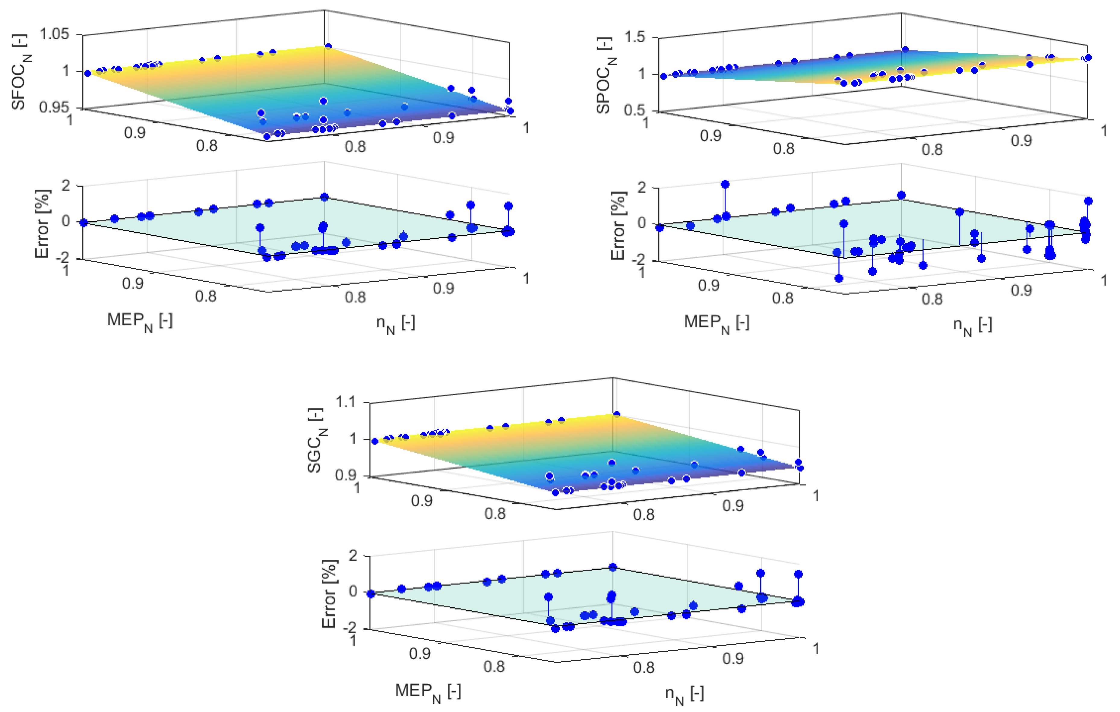
2.1. Specific Fuel Consumption at SMCR

Firstly, specific fuel consumptions at SMCR were divided by themselves at the nominal maximum continuous rating (NMCR) to obtain the normalized specific fuel consumptions regarding NMCR: SFOC${}_N$, SGC${}_N$ and SPOC${}_N$. Equation (1) mathematically describes this procedure for each one of the normalized specific fuel consumption (SFC${}_N$). In this equation, $P_B$ is brake power [kW]; j varies from 1 to 4, representing the SMCR position (L1, L2, L3, and L4); and k varies from 1 to 22, representing the engines. Then, regressions were performed as a function of mean effective pressure and engine speed, normalized with respect to NMCR (MEP${}_N$ and $n_N$), as respectively defined by Equations (2) and (3). Mean effective pressure may also be written as in Equation (4) [29]. Therefore, knowing that the number of cylinders ($Z_c$), revolutions of crankshaft per complete working cycle (r), and cylinder swept volume ($V_S$) are engine constants, MEP${}_N$ could also be written as in Equation (5). Hence, $n_N$ and MEP${}_N$ could be calculated with the support of Table 1.

$$SF{C}_{N,jk}=\frac{SF{C}_{SMCR,jk}}{SF{C}_{NMCR,k}}$$

(1)

$$ME{P}_{N,jk}=\frac{ME{P}_{SMCR,jk}}{ME{P}_{NMCR,k}}$$

(2)

$$n_{N,jk}=\frac{n_{SMCR,jk}}{n_{NMCR,k}}$$

(3)

$$MEP=\frac{r}{Z_c·V_S}·\frac{P_B}{n}$$

(4)

$$ME{P}_{N,jk}=\frac{P_{SMCR,jk}}{n_{SMCR,jk}}·\frac{n_{NMCR,k}}{P_{NMCR,k}}$$

(5)

The polynomial surfaces obtained for specific fuel consumptions at SMCR normalized with respect to NMCR and their percentage errors of regression are illustrated in Figure 1. As it can be seen, normalized specific fuel consumptions vary almost linearly with respect to MEP${}_N$ and are practically not influenced by $n_N$, such that they could be approached by plans. Moreover, engines of type G and S did not present substantial differences from each other and, for this reason, they were analyzed together. The largest deviations were 1.3%, 1.9%, and 1.4% for SFOC${}_N$, SPOC${}_N$, and SGC${}_N$, respectively, showing that the polynomials achieved were suitable. In order to reproduce the polynomial surfaces,

Table 2. Coefficients of the polynomial surfaces.

Coefficients	SFOC${}_{\mathit{N}}$	SPOC${}_{\mathit{N}}$	SGC${}_{\mathit{N}}$
$a_{00}$	0.8342	2.294	0.7870
$a_{10}$	−0.0009009	−0.0006027	−0.000691
$a_{01}$	0.1665	−1.296	0.2136

provides the coefficients (a) for each one of the normalized specific fuel consumptions formulated as in Equation (6).

$$SF{C}_N=a_{00}+a_{10}·n_N+a_{01}·ME{P}_N$$

(6)

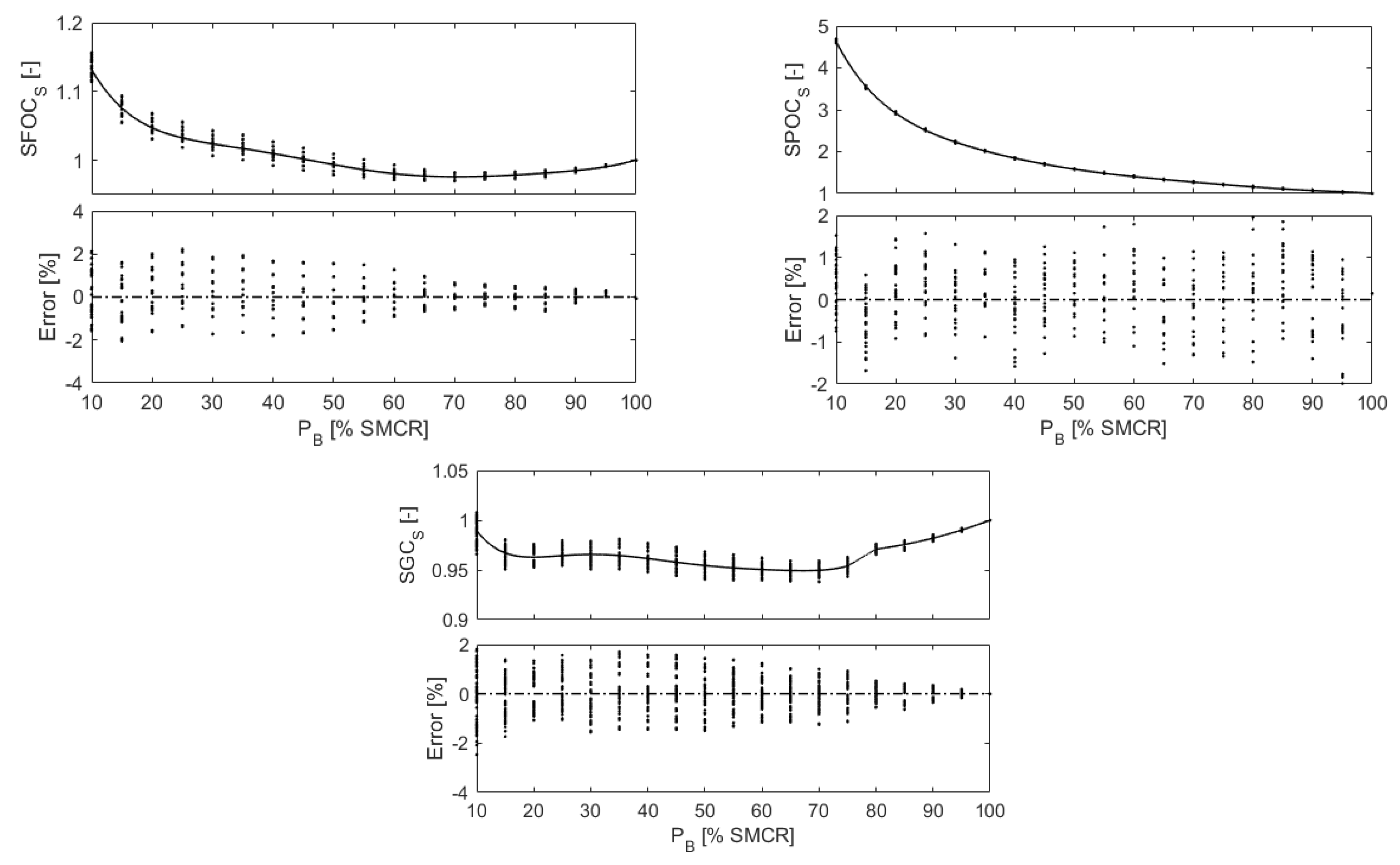
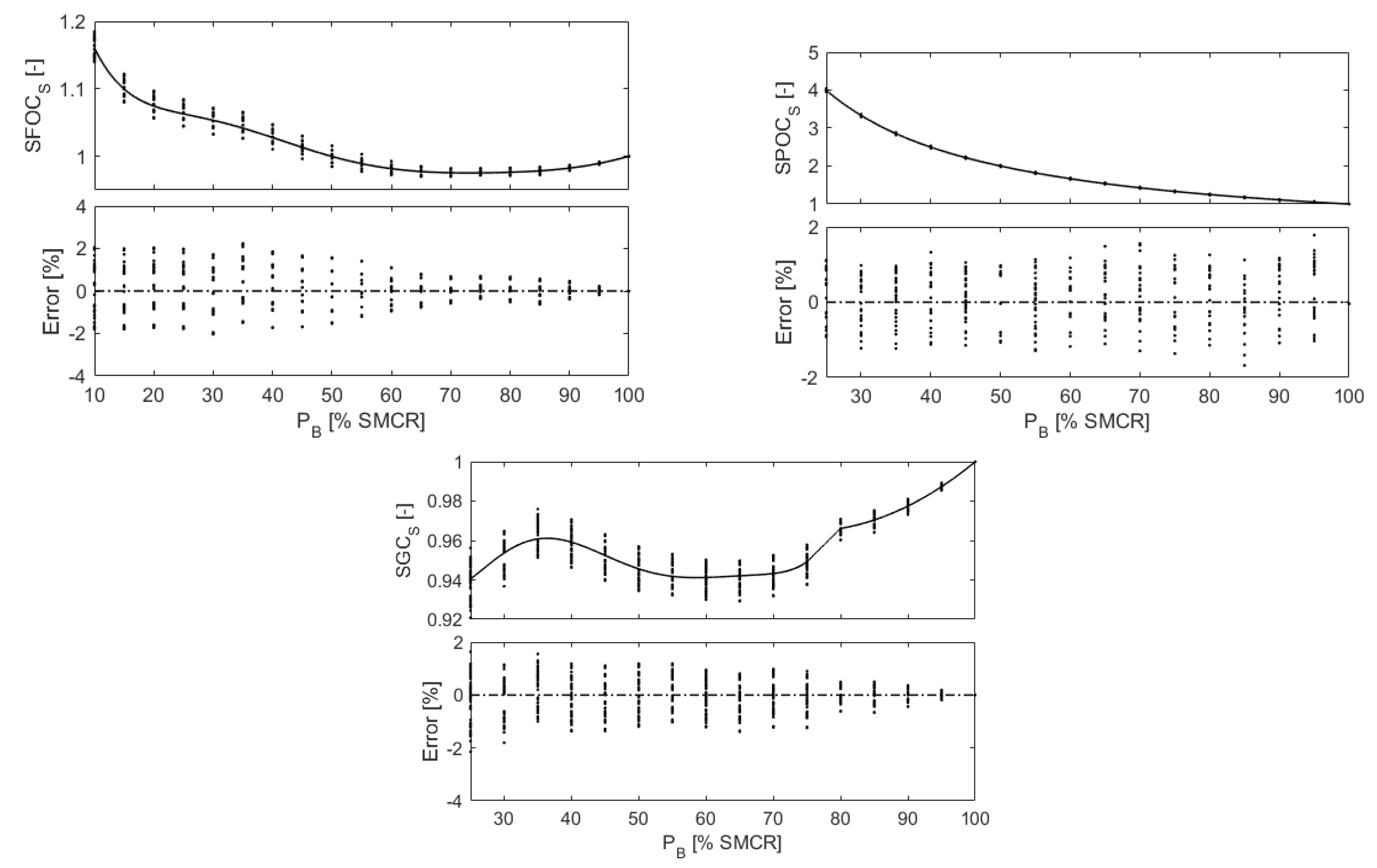
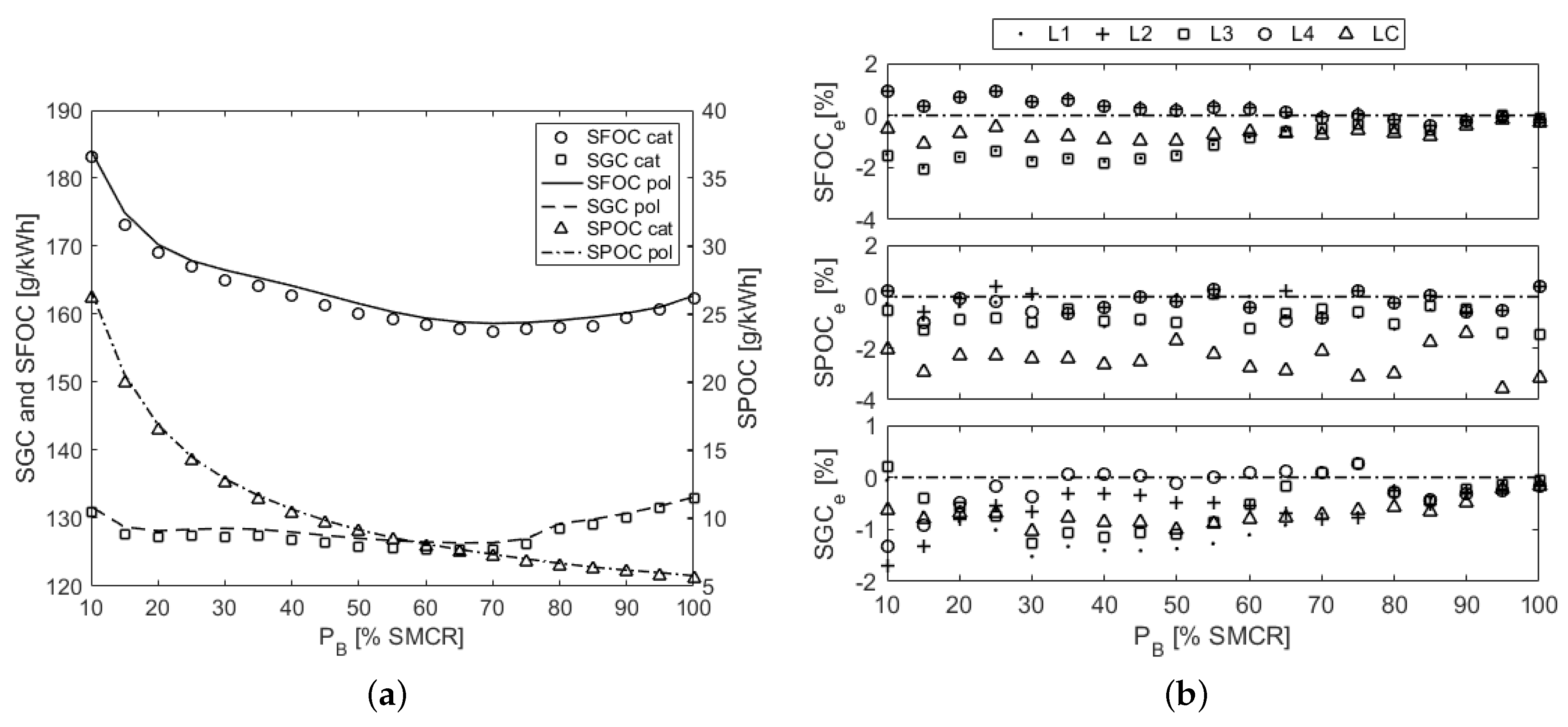
2.2. Specific Fuel Consumption at Part Load

The normalized specific fuel consumptions with respect to SMCR (SFOC${}_S$, SGC${}_S$, SPOC${}_S$) were achieved by dividing their values at part load by themselves at SMCR. Equation (7) exemplifies this procedure for a generic normalized specific fuel consumption (SFC${}_S$), where the index i varies from 1 to 19, representing engine loads from 10 to 100% with 5% step; j varies between 1 and 4 representing the SMCR position; and k varies between 1 and 22, representing the engines.

$$SF{C}_{S,ijk}=\frac{SF{C}_{ijk}}{SF{C}_{SMCR,jk}}$$

(7)

A compromise between simplicity and accuracy was pursued to develop really fast and useful modelling. Thus, polynomials with degrees from one to nine were tested, and the one presenting the best fitting was selected. In some cases, the data set presented discontinuities too sharp to be captured by only one polynomial curve, even of a high order. Instead, two and three polynomials of a low order presented better fittings and were preferred in such cases.

Figure 2 and Figure 3 show the normalized curves and their percentage errors of regression as a function of brake power given in a percentage of SMCR ($P_B[\%SMCR]$) for FPP and CPP driving, respectively. The specific fuel consumptions hold distinct behaviours from one another and, consequently, they were approximated by polynomials of different degrees. Furthermore, for a better approximation of the SGC${}_S$ trend, three polynomials were employed. The driving type is not very influential on the form of the curves except on the SGC${}_S$, which has slightly different behaviours for FPP and CPP driving. In general, the mismatches rise as engine load decreases, except regarding SPOC${}_S$, whose errors are quite dispersed over the load range analyzed. Regarding FPP driving, the largest errors were 2.2%, −2.0%, and −2.5%, respectively for SFOC${}_S$, SPOC${}_S$, and SGC${}_S$ (Figure 2). Similarly, the largest errors regarding CPP driving were 2.2%, 1.8%, and −2.1%, respectively for SFOC${}_S$, SPOC${}_S$, and SGC${}_S$ (Figure 3).

All polynomial curves were obtained by using centring and scaling transformation to improve the numerical properties of both the polynomial and fitting algorithms.

Table 3. Coefficients of the polynomial curves.

Driving	Coefficients	SFOC${}_{\mathit{S}}$	SPOC${}_{\mathit{S}}$	SGC${}_{\mathit{S}}$
				a	b	c
	$a_0$ *	986.3	1484	959.6	962.4	982.0
	$a_1$ *	−36.64	−486.5	−15.06	11.91	10.34
	$a_2$ *	25.25	256.4	−0.4842	0	1.730
	$a_3$ *	20.94	−134.4	12.56	0	0
FPP	$a_4$ *	−13.29	−47.19	−5.405	0	0
	$a_5$ *	−8.209	36.87	−4.242	0	0
	$a_6$ *	5.533	49.79	2.848	0	0
	$a_7$ *	0	−26.58	0	0	0
	$\mu$	55.00	55.00	42.50	77.50	90.00
	$\sigma$	27.39	27.39	20.16	3.536	7.079
	$a_0$ *	989	1599	945.6	957.7	977.5
	$a_1$ *	−49.71	−596.8	−17.73	11.95	11.99
	$a_2$ *	50.68	221.8	16.44	0	2.789
	$a_3$ *	4.908	−62.2	9.05	0	0
CPP	$a_4$ *	−31.54	20.48	−13.56	0	0
	$a_5$ *	7.997	−22.79	−0.3384	0	0
	$a_6$ *	9.374	9.135	2.745	0	0
	$a_7$ *	−3.594	0	0	0	0
	$\mu$	55.00	55.00	42.50	77.50	90.00
	$\sigma$	27.39	27.39	20.16	3.536	7.079

* These coefficient’s values are multiplied by 1000.

provides the coefficients (a) for the formulation given in Equation (8), in which x is a function of load [% SMCR], mean ($\mu$), and standard deviation ($\sigma$) of the applicable load range, as given in Equation (9). As the SGC${}_S$ was approached by three polynomials, the letters “a”, “b”, and “c” in this table indicate the load range where each polynomial is applicable. Thus, these letters indicate, respectively, load ranges from 10 to 70%, 70 to 80%, and 80 to 100%.

$$SF{C}_S=a_0+a_1·x+a_2·x^2+a_3·x^3+\dots +a_7·x^7$$

(8)

$$x=\frac{P_B[\%SMCR]-\mu [\%SMCR]}{\sigma [\%SMCR]}$$

(9)

3. Model

The model relies on computing the specific fuel consumptions for any SMCR and any part load by means of Equation (10). Consequently, the polynomials previously given by Equations (6) and (8) and the coefficients listed in Table 2 must be used. To use these equations, it is also necessary to consider Table 1 to calculate MEP${}_N$ and $n_N$, respectively by Equations (3) and (5) for a certain engine and SMCR. Additionally, the specific fuel consumptions at NMCR (SFOC${}_{NMCR}$, SPOC${}_{NMCR}$, and SGC${}_{NMCR}$) for every single engine are necessary and, for this reason, they are listed in

Table 4. Specific fuel consumptions at NMCR [g/kWh].

Engine	SFOC${}_{\mathit{NMCR}}$	SPOC${}_{\mathit{NMCR}}$	SGC${}_{\mathit{NMCR}}$
G95ME-C9.6	165.0	4.9	135.9
G95ME-C10.5	163.0	4.9	134.2
G95ME-C9.5	166.0	5.0	136.7
G90ME-C10.5	165.0	4.9	135.9
S90ME-C10.5	166.0	5.0	136.7
G80ME-C9.5	166.0	5.0	136.7
S80ME-C9.5	166.0	5.0	136.7
G70ME-C10.5	163.0	5.5	133.7
G70ME-C9.5	167.0	5.0	137.5
S70ME-C10.5	166.0	5.0	136.7
S70ME-C8.5	169.0	5.0	139.2
S65ME-C8.5	169.0	5.0	139.2
G60ME-C9.5	167.0	5.0	137.5
S60ME-C10.5	166.0	5.0	136.7
S60ME-C8.5	169.0	5.0	139.2
G50ME-C9.6	167.0	5.0	137.5
S50ME-C9.7	165.0	4.9	135.9
S50ME-C9.6	167.0	5.0	137.5
S50ME-C8.5	170.0	5.1	140.0
G45ME-C9.5	170.0	5.1	140.0
G40ME-C9.5	174.0	5.2	143.3
S40ME-C9.5	172.0	5.1	141.7

. The only difference between FPP and CPP driving is the coefficients’ values of the polynomial SFC${}_S$.

$$SFC=SF{C}_{NMCR}·SF{C}_N·SF{C}_S$$

(10)

4. Results and Discussion

In order to investigate the accuracy of the approach proposed in this paper, two engines of intermediary NMCR were simulated, and the results were compared with catalogue data [28]. As the polynomials were obtained considering SMCR on L1, L2, L3, and L4, it was necessary to investigate the approach accuracy for intermediate points. Therefore, the SMCR was additionally placed on the center of engine layout diagrams (LC), such that the engine 9G80ME-C9.5-GI was examined for an SMCR of 33,571 kW and 65 rpm, and the engine 5S50ME-C9.6-GI was examined for an SMCR of 7037 kW and 103 rpm.

Figure 4 illustrates the qualitative and quantitative performance of the developed approach employed on the engine 9G80ME-C9.5-GI driving a fixed pitch propeller. It is noticeable in Figure 4a that the polynomials are able to predict the behaviour of SFOC, SPOC, and SGC with only minor mismatches, even when SMCR is in the center of the layout diagram (LC). Although the SMCR was not placed on LC in the regression process, the biggest deviations did not occur for LC, except regarding specific pilot oil consumption (SPOC${}_e$), achieving −3.6% at 95% load, as it can be seen in Figure 4b. The percentage error for the specific fuel oil consumption (SFOC${}_e$) peaked at −2.0% when SMCR was on L3, and the load was 15% of SMCR. Also in a low load, the percentage error for the specific gas consumption (SGC${}_e$) peaked at −1.7% when SMCR was on L2 and the load was 10% of SMCR.

Qualitative and quantitative performances of the developed approach employed on the engine 5S50ME-C9.6-GI driving a controllable pitch propeller is illustrated in Figure 5. As in Figure 4a, it is noted by Figure 5a that the polynomials are able to predict the behaviour of specific fuel consumptions for SMCR in the center of the layout diagram (LC) also for this engine and CPP driving. Likewise, the biggest deviations did not occur for LC, except regarding SPOC${}_e$, achieving −2.8% at 100% load, as it can be seen in Figure 5b. The percentage error SFOC${}_e$ peaked at −2.0% when SMCR was on L1 and the load was 30% of SMCR. Either for 25% or 65% of SMCR, SGC${}_e$ achieved −1.6% when SMCR was on L2.

5. Conclusions

The present study has provided state-of-the-art modelling of marine engines and ship energy systems, and also addressed programming languages and dedicated applications to be employed in these areas. Moreover, a simple and fast model to assist in tackling optimization problems involving the selection of dual-fuel two-stroke Diesel engines was developed. The model was implemented in a MatLab environment and relies on normalizing specific fuel consumptions and approximating their trends by polynomials. Since the behaviour of marine engines driving fixed and controllable pitch propellers has been taken into account, different polynomials were derived.

Finally, the comparison between the model predictions and catalogue data for two engines of different sizes driving different propeller types revealed that the model was capable of adequately representing the behaviour of the specific fuel consumptions. The majority of the deviations was negative, meaning that the model overestimated the specific fuel consumptions of those engines. The greatest deviation did not exceed −3.6%, even when the specified maximum continuous rating was placed in the center of the layout diagram. Having this scenario was quite acceptable, and the model may be used successfully whenever one is interested in a fast and easy way to obtain specific fuel consumptions of several engines, such as in optimization problems.

References

1. Thomson, H.; Corbett, J.J.; Winebrake, J.J. Natural gas as a marine fuel. Energy Policy 2015, 87, 153–167. [Google Scholar] [CrossRef] [Green Version]
2. IMO. Resolution MEPC.176(58): Amendments to the Annex of the Protocol of 1997 to Amend the International Convention for the Prevention of Pollution from Ships, 1973, as Modified by the Protocol of 1978 Relating Thereto. 2008. Available online: http://www.imo.org/en/KnowledgeCentre/IndexofIMOResolutions/Marine-Environment-Protection-Committee-%28MEPC%29/Documents/MEPC.176%2858%29.pdf (accessed on 3 October 2018).
3. IMO. IMO Sets 2020 Date for Ships to Comply with Low Sulphur Fuel Oil Requirement. 2016. Available online: http://www.imo.org/en/MediaCentre/PressBriefings/Pages/MEPC-70-2020sulphur.aspx (accessed on 3 October 2018).
4. DNV-GL. Sulphur Cap Ahead—Time to Take Action. Available online: https://www.dnvgl.com/article/sulphur-cap-ahead-time-to-take-action-94198 (accessed on 3 October 2018).
5. Karim, G. Dual-Fuel Diesel Engines; CRC Press: Boca Raton, FL, USA, 2015. [Google Scholar]
6. Caton, J.A. (Ed.) An Introduction to Thermodynamic Cycle Simulations for Internal Combustion Engines; John Wiley & Sons, Ltd.: Hoboken, NJ, USA, 2015. [Google Scholar] [CrossRef]
7. Schulten, P.J.M. The Interaction Between Diesel Engines, Ship and Propellers During Manoeuvring. Ph.D. Thesis, Delft University of Technology, Delft, The Netherlands, 2005. [Google Scholar]
8. Hountalas, D.T. Prediction of marine diesel engine performance under fault conditions. Appl. Therm. Eng. 2000, 20, 1753–1783. [Google Scholar] [CrossRef]
9. Rakopoulos, C.; Dimaratos, A.; Giakoumis, E.; Rakopoulos, D. Evaluation of the effect of engine, load and turbocharger parameters on transient emissions of diesel engine. Energy Convers. Manag. 2009, 50, 2381–2393. [Google Scholar] [CrossRef]
10. Scappin, F.; Stefansson, S.H.; Haglind, F.; Andreasen, A.; Larsen, U. Validation of a zero-dimensional model for prediction of NOx and engine performance for electronically controlled marine two-stroke diesel engines. Appl. Therm. Eng. 2012, 37, 344–352. [Google Scholar] [CrossRef]
11. Cordtz, R.; Schramm, J.; Andreasen, A.; Eskildsen, S.S.; Mayer, S. Modeling the Distribution of Sulfur Compounds in a Large Two Stroke Diesel Engine. Energy Fuels 2013, 27, 1652–1660. [Google Scholar] [CrossRef]
12. Raptotasios, S.I.; Sakellaridis, N.F.; Papagiannakis, R.G.; Hountalas, D.T. Application of a multi-zone combustion model to investigate the NOx reduction potential of two-stroke marine diesel engines using EGR. Appl. Energy 2015, 157, 814–823. [Google Scholar] [CrossRef]
13. Payri, F.; Olmeda, P.; Martín, J.; García, A. A complete 0D thermodynamic predictive model for direct injection diesel engines. Appl. Energy 2011, 88, 4632–4641. [Google Scholar] [CrossRef]
14. Cordtz, R.; Mayer, S.; Eskildsen, S.S.; Schramm, J. Modeling the condensation of sulfuric acid and water on the cylinder liner of a large two-stroke marine diesel engine. J. Mar. Sci. Technol. 2017, 23, 178–187. [Google Scholar] [CrossRef] [Green Version]
15. Gugulothu, S.; Reddy, K. CFD simulation of in-cylinder flow on different piston bowl geometries in a DI diesel engine. J. Appl. Fluid Mech. 2016, 9, 1147–1155. [Google Scholar] [CrossRef]
16. Pang, K.M.; Karvounis, N.; Walther, J.H.; Schramm, J. Numerical investigation of soot formation and oxidation processes under large two-stroke marine diesel engine-like conditions using integrated CFD-chemical kinetics. Appl. Energy 2016, 169, 874–887. [Google Scholar] [CrossRef] [Green Version]
17. Sun, X.; Liang, X.; Shu, G.; Lin, J.; Wang, Y.; Wang, Y. Numerical investigation of two-stroke marine diesel engine emissions using exhaust gas recirculation at different injection time. Ocean Eng. 2017, 144, 90–97. [Google Scholar] [CrossRef]
18. Benvenuto, G.; Carrera, G.; Rizzuto, E. Dynamic Simulation of Marine Propulsion Plants. In Proceedings of the International Conference on Ship and Marine Research, Rome, Italy, 5–7 October 1994. [Google Scholar]
19. Kyrtatos, N.P.; Theodossopoulos, P.; Theotokatos, G.; Xiros, N. Simulation of the overall ship propulsion plant for performance prediction and control. In Proceedings of the Conference on Advanced Marine Machinery Systems with Low Pollution and High Efficiency, Newcastle upon Tyne, UK, 25–26 March 1999. [Google Scholar]
20. Theotokatos, G.P. Ship Propulsion Plant Transient Response Investigation using a Mean Value Engine Model. Int. J. Energy 2008, 2, 66–74. [Google Scholar]
21. Stapersma, D.; Vrijdag, A. Linearisation of a ship propulsion system model. Ocean Eng. 2017, 142, 441–457. [Google Scholar] [CrossRef]
22. Michalski, J. A method for selection of parameters of ship propulsion system fitted with compromise screw propeller. Pol. Marit. Res. 2007, 14. [Google Scholar] [CrossRef]
23. Aldous, L.; Smith, T. Speed Optimisation for Liquefied Natural Gas Carriers: A Techno-Economic Model. In Proceedings of the International Conference on Technologies, Operations, Logistics & Modelling for Low Carbon Shipping, Newcastle, UK, 11–12 September 2012. [Google Scholar]
24. Talluri, L.; Nalianda, D.; Kyprianidis, K.; Nikolaidis, T.; Pilidis, P. Techno economic and environmental assessment of wind assisted marine propulsion systems. Ocean Eng. 2016, 121, 301–311. [Google Scholar] [CrossRef] [Green Version]
25. Sakalis, G.N.; Frangopoulos, C.A. Intertemporal optimization of synthesis, design and operation of integrated energy systems of ships: General method and application on a system with Diesel main engines. Appl. Energy 2018, 226, 991–1008. [Google Scholar] [CrossRef]
26. Trivyza, N.L.; Rentizelas, A.; Theotokatos, G. A novel multi-objective decision support method for ship energy systems synthesis to enhance sustainability. Energy Convers. Manag. 2018, 168, 128–149. [Google Scholar] [CrossRef]
27. Shi, W.; Grimmelius, H.T.; Stapersma, D. Analysis of ship propulsion system behaviour and the impact on fuel consumption. Int. Shipbuild. Prog. 2010, 57, 35–64. [Google Scholar] [CrossRef]
28. MAN Diesel & Turbo. Computerised Engine Application System-Engine Room Dimensioning (CEAS-ERD); MAN Diesel & Turbo: Munich, Germany, 2018. [Google Scholar]
29. Woud, H.K.; Stapersma, D. Design of Propulsion and Electric Power Generation Systems; IMarEST: London, UK, 2013. [Google Scholar]
30. Woodyard, D. Pounder’s Marine Diesel Engines and Gas Turbines; Elsevier BV: Oxford, UK, 2009. [Google Scholar]
Figure 1. Polynomial surfaces of the specific fuel consumptions normalized with respect to the nominal maximum continuous rating (NMCR) and respective percentage errors of regression.
Jmse 07 00020 g001
Figure 2. Polynomial curves of the specific fuel consumptions normalized with respect to specified maximum continuous rating (SMCR) and respective percentage errors of regression for fixed pitch propeller (FPP) driving.
Jmse 07 00020 g002
Figure 3. Polynomial curves of the specific fuel consumptions normalized with respect to SMCR and respective percentage errors of regression for controllable pitch propeller (CPP) driving.
Jmse 07 00020 g003
Figure 4. Qualitative and quantitative performance of the developed approach for the engine 9G80ME-C9.5-GI driving a fixed pitch propeller. (a) Qualitative comparison for the SMCR in the center of the layout diagram (LC). (b) Quantitative comparison for the SMCR in five different positions.
Jmse 07 00020 g004
Figure 5. Qualitative and quantitative performance of the developed approach for the engine 5S50ME-C9.6-GI driving a controllable pitch propeller. (a) Qualitative comparison for the SMCR in the center of the layout diagram (LC). (b) Quantitative comparison for the SMCR in five different positions.
Jmse 07 00020 g005