1. Introduction
The knowledge of the hydro- and morphodynamics induced by a slender vertical pile is very important for the design of marine structures, such as offshore platforms or wind farms. In particular, the evaluation of the scour at the base of the cylinder and the force acting on it is fundamental for a correct design of a marine structure. The present topics have been experimentally and numerically studied in the literature. The pioneering work of Morison [
1] started an extensive series of studies on the forces over vertical piles under waves. Suddenly, Keulegan and Carpenter [
2] found that those processes are highly influenced by a nondimensional parameter (named the Keulegan-Carpenter number
KC) that depends on, among the others, the particle velocity and on the pile diameter. Scour process in river hydraulics has been extensively studied because of its importance on bridge failure; however, this process in coastal and offshore engineering has not received the same attention. The work of Herbich [
3] was the first important contribution to the knowledge of the hydrodynamic processes in marine environment. From the 1990s, several studies on the hydrodynamics have been realized [
4,
5,
6,
7], mostly focusing on the analysis of the scour process and the formation of vortices. Sumer et al. [
4,
5] observed that the vortex flow regimes for a free cylinder subjected to an oscillatory flow and the lee-wake vortex flow are governed primarily by
KC. The bed shear stress under the horseshoe vortex and the bed shear stress in the lee wake are also influenced by
KC. Olsen and Kjellesvig [
6] simulated the scour process in clear water regime by employing the
k-ε turbulence model. Roulund et al. [
7] studied numerically the live-bed scour for cohesionless sediment by making use of Reynolds-averaged Navier–Stokes (RANS) equations with a
k-ω closure model. Subsequently, Baykal et al. [
8] incorporated the effects of lee-wake vortices, as well as suspended sediment transport. In the majority of the works the forcing was either current or combined wave and current; however, in a number of instances, the tidal range was significantly smaller than the wave height at breaking [
9]. So waves became significant with respect to current and, hence, the flow forcing was only due to waves. In the present paper, the focus was on the analysis of the hydrodynamics around a vertical slender cylinder subjected to wave forcing only, by making use of both the experimental and numerical models. In particular, the direct numerical simulation (DNS) approach was used. The numerical results were compared with the experimental data. The combined analysis focused on the pressure distributions around the pile and on the evaluation of the total force on it at different wave phases. The total force acting on the pile was also compared with the widely used Morison formula [
1] and a discussion on the applicability of such formula for nonlinear waves has been provided. Moreover, the wall shear stress induced by the waves around the cylinder and the analysis of the streamlines connected with the vortex pattern evolution around the cylinder allowed us to explain the movement of sand particles and the seabed morphology. In conclusion, in the present paper the authors exploited the different information provided by the numerical and experimental approaches in order to shed light on relevant physical processes which would be otherwise difficult to understand by using solely experimental or numerical data.
2. Experimental Setup
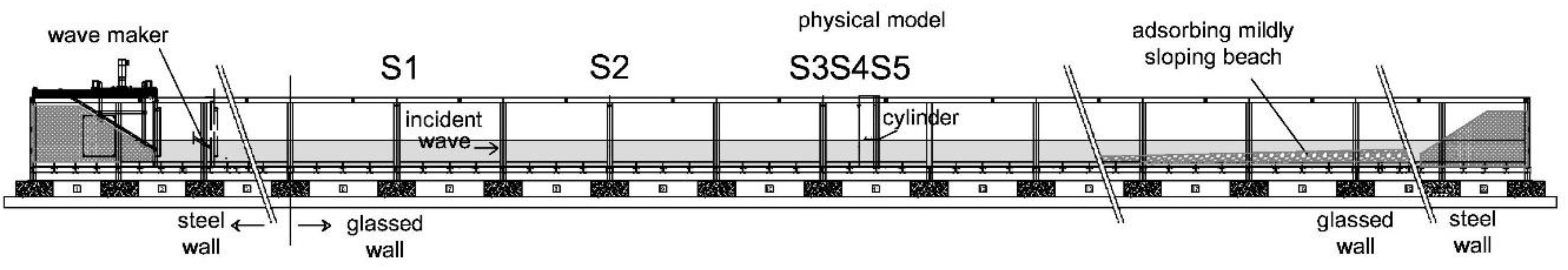
The experiments were carried out at the wave flume of the Hydraulics and Maritime Construction Laboratory of the Università Politecnica delle Marche (Ancona, Italy). The channel is 50-m long, 1-m wide, and 1.3-m high. The flow motion was forced by regular waves (Stokes I order theory) generated by a piston-type wavemaker. An adsorbing mildly sloping beach (slope 1:20) made of coarse gravel was used to reduce the wave reflection and to guarantee an undisturbed flow in the measuring area. The reflection was studied and considered negligible (<5%). The side walls of the flume were glassed for the central 36 m and enabled one to video record and carry out optical measurements.
Two different experimental campaigns were performed. The former experimental campaign aimed to investigate the bottom morphology induced by the presence of a vertical slender pile under regular and random wave action in live-bed regime. Several wave tests were performed as a combination of different wave heights
H, wave periods
T, and water depths
h. The detailed description of the mobile-bed experiments and the analysis of the results were reported in Corvaro et al. [
10]. Recently, a second experimental campaign was realized for a deeper analysis of the hydrodynamics around the pile induced by regular waves. Even for this experimental campaign, several wave tests, characterized by different combinations of the wave heights, periods, and water depths, were studied.
Since the purpose of the present analysis was that of characterizing the hydrodynamics around a vertical slender cylinder, we here analyzed one specific regular wave that evolved over a rigid bed with a water depth
h = 0.35 m, a wave height
H of 0.10 m, a wave period
T of 1.77 s, and a wave length
L of 3.0 m. The Keulegan–Carpenter parameter, defined as
KC = UmT/D (
Um is the maximum velocity at the bottom just outside of the boundary layer and
D is the diameter of the pile), is
KC ≈ 6 and the Reynolds number, defined as
Re = UmA/ν (A is the semi-amplitude of the horizontal motion of the water particles just outside of the bottom boundary layer,
ν is the kinematic viscosity), is
Re ≈ 3 × 10
4. Due to the significant computational cost, we focused on one specific forcing condition characterized by vorticity generation and scour formation, as found in the first experimental campaign [
10] for waves with similar values of a Keulegan–Carpenter parameter. Being the vortex flow regimes governed primarily by
KC for a cylinder subjected to an oscillatory flow [
5], the wave here analyzed was representative of waves within the vortex shedding flow regime. The scour pattern map obtained in the previous experiments [
10] was here used in order to relate it with the vortical structures.
The water level evolutions, and thus wave heights, at different locations of the flume were measured and monitored by five electro-sensitive elevation gauges (see
Figure 1). They were located as follows: S1 just downstream of the wave paddle at a distance of 8.43 m, S2 at 12.43 m, S3 at 16.43 m, S4 at 16.83 m, and S5 at 17.15 m, in correspondence to the cylinder.
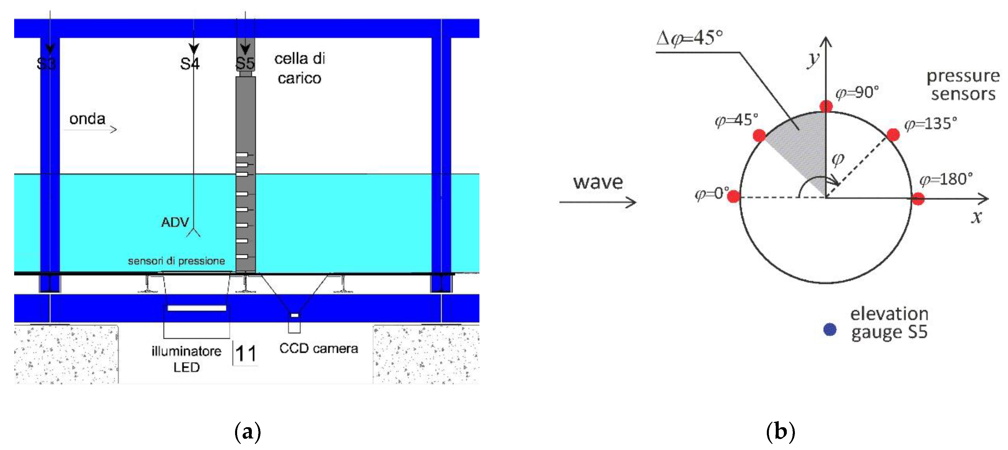
The sketch of the physical model (rigid bed) is shown in
Figure 2a. A Cartesian coordinate system
x, y, z was used. The origin was placed in the centre of the pile at the bottom of the flume, the
x-axis was in the direction of the flow with the wave propagating from negative to positive values, the
y-axis was horizontal and transversal to the incoming wave direction (see
Figure 2b for the plan view of the coordinate system) and the vertical
z-axis, coinciding with the pile’s axis, pointed upward.
In the mobile-bed experiments a steel pile with a dimeter
D = 0.10 m was fitted in the sandy seabed. In order to measure the pressure distribution around the cylinder at different water depths, in the rigid-bed experiments a PVC pile (PolyVinyl Chloride) was used because the housing of the pressure sensors along the vertical was easier by using a plastic material with respect to the steel. The pile was connected at the bottom by means of a hinge that allowed the complete rotation of the pile around its axis. The cylinder, being moment free around the hinge, was ensured in the equilibrium condition at the top of the pile by means of a biaxial load cell (P500.BIAX-S/400N, Deltatech, Sogliano al Rubicone, FC, Italy) for the total force measurement. Four pressure sensors Keller 23Y were embedded in the pile along the same vertical (
z = 0.01 m,
z = 0.08 m,
z = 0.16 m, and
z = 0.24 m). In order to obtain a good estimate of the pressure distribution around the cylinder, the pile was rotated by incremental angles
Δφ around its vertical axis (see
Figure 2b) allowing it to collect the data with a good discretization of the pile surface. Hence, each wave test was repeated more times from
φ = 0° to
φ = 180° with an angle
Δφ = 45
°. The locations where the pressure was monitored in the numerical model are at
φ = 0°,
φ = 90°,
φ = 180°, and
φ = 270° and vertical depths
z = 0.00–0.32 m (every 0.08 m). Furthermore, the local water particle velocity was measured by means of an acoustic Doppler velocimetry (ADV) placed in front of the pile (
φ = 0°), in the lateral side (
φ = 90°) and behind it (
φ = 180°) at different depths (
z = 0.01 m,
z = 0.08 m,
z = 0.16 m,
z = 0.24 m). In the numerical model, the velocity was monitored at
φ = 0°,
φ = 90°,
φ = 180°, and
φ = 270° and at vertical depths
z = 0.00–0.32 m (every 0.08 m). The elevation gauge S5 was placed in correspondence with the pile in order to measure the water level in its section and to synchronize the pressure recordings over different tests (
Figure 2).
3. Numerical Setup
The approach used in this study to solve the Navier–Stokes equations consisted of in a direct numerical simulation (DNS) modelling conducted by using the commercial software ANSYS Fluent. Space and time were discretized and the resulting equations were numerically solved without any turbulence model. Increasing the Reynolds number Re, the turbulent scales became smaller and smaller both in space and time; therefore, fine grids and small time steps were needed. The DNS solved all the scales of the motion, from the integral scale to the smallest dissipative one (Kolmogorov’s scale). Therefore, the accuracy obtained with this model was the highest possible (compared to large eddy simulations or to RANS equations closed by a turbulence model) with the disadvantage of a huge computational cost, even at low Reynolds numbers like those considered in this work (as above reported, the wave was characterized by a Reynold number Re ≈ 3 × 10⁴). Note that here the Re number was defined according to the maximum velocity Um (as usually done for flow induced by waves) and not according to the mean velocity value, which was almost null in an oscillatory flow. From the practical point of view, we found that the computational resources required by DNS are large but significantly lower than those usually adopted for solving a different flow problem (e.g., current) characterized by a similar Re value which was obtained by using the mean velocity. The employed discretization scheme adopted a finite volume method in space and an implicit algorithm in time. More in detail, it used a second order backward time integration scheme, while a second order reconstruction of the numerical fluxes at faces yields a second order accuracy also in space. The volume of fluid (VOF) method was used for locating and tracking the free surface. It consisted of the assumption that the two-phase flow was a mixed fluid whose density and viscosity were weighted functions of the volume fraction which evaluated the fraction of the volume occupied by the two phases and was computed by an advection equation.
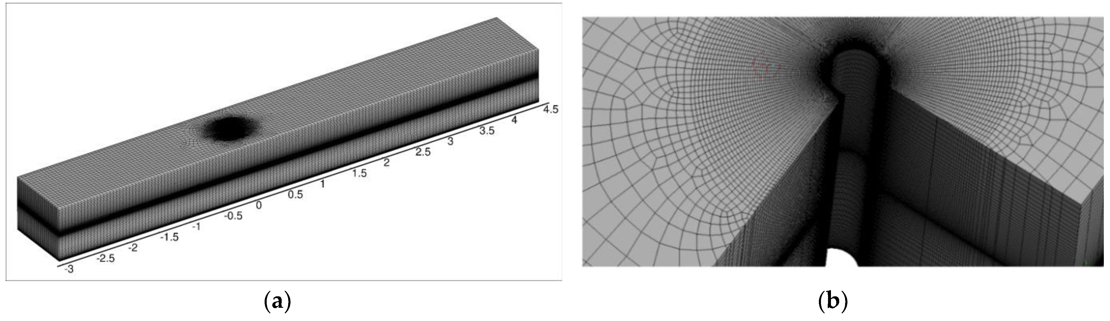
The solved wave flume was 1-m wide, 6–7.5 m long, and 0.8-m height. The cylinder had a diameter of 0.1 m and it was placed 3 m downstream the inlet boundary condition. A no-slip boundary condition was applied in the bottom and lateral boundaries of the domain, while at the top and outer boundaries the hydrostatic pressure was imposed. Close to the outlet of the bigger, 7.5-m-long domain, a 1.5-m-long absorption zone, called “numerical beach”, was employed. The approach used the last portion of the numerical domain to damp the downstream propagation of the waves by adding a sink term in the vertical component of the momentum equations. This term depended on the vertical velocity and its strength rose with the value of the distance from both the free surface and the interface between the true domain of interest and the absorption zone [
11]. Finally, at the inlet, a time-dependent Dirichlet condition was imposed which enforced the creation of waves of different types, according to the Stokes theory, and intensity. A regular wave was forced with a Stokes I order theory with the same characteristics of the one reproduced in the experimental test (
H = 0.10 m,
T = 1.77 s,
h = 0.35 m, and
L = 3.0 m). The numerical simulation of the regular wave was performed with a fixed
dt = 0.01 s, a coupled solver for the discretized equations and with different grid densities. In the zone surrounding the pile (located at 3 m from the inlet), at the bottom and close to the free surface, the grid was clustered to adequately resolve the boundary layer and the position of the interface between the two fluids, see
Figure 3.
3.1. Sensitivity Analysis
The sensitivity of the numerical solution with respect to the mesh resolution was analyzed by means of 6 different grids, two of them 6-m-long and the remaining 7.5-m-long. The characteristics of the grids are summarized in
Table 1. To give an idea of the computational costs, the simulation with the largest number of volumes required more than a month by using a small Linux cluster consisting of 32 Intel Xeon E5 2620 v4 cores running at 2.1 GHz.
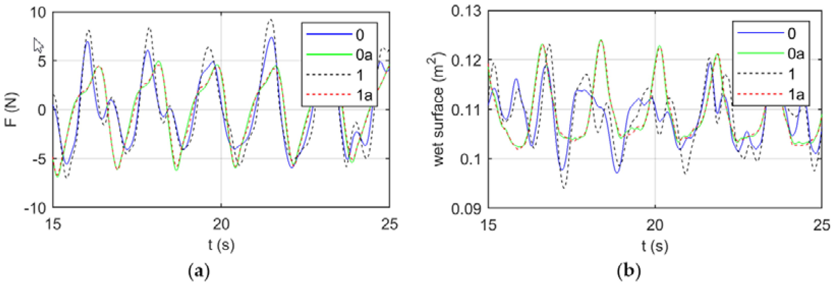
In order to analyze the effectiveness of the adoption of the numerical beach, in
Figure 4 we report the behavior of the force over the pile and of the wet surface around it for simulations 0 and 0a (continuous lines) and 1 and 1a (dashed lines) where the suffix
“a” represents the use of the numerical beach. The use of the absorption zone drastically changed the results, thus highlighting the effectiveness of the approach. From one side, a significant reduction and regularization of the force acting on the pile was observed. From the other, the wet surface did not show a superposition of different types of waves by using the absorption zone. Indeed, these smaller and irregular waves we a result of wave reflection at the end of the finite numerical domain and an increase in terms of resolution did not lead to a more stable result when no absorption zone was used.
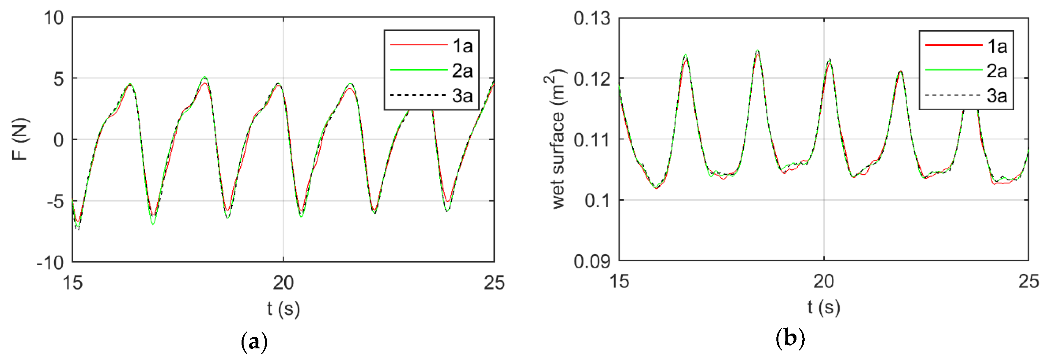
To perform an analysis of sensibility of the grid resolution, the force over the cylinder in the direction of wave propagation was analyzed. As shown in
Figure 5a, the solved oscillation of the streamwise force over the pile changed by increasing the mesh resolution from the case 1a to 3a. Note that even if the number of elements of the grid 2a was only slightly larger than those of the grid 1a, the first was significantly refined in the boundary layer around the pile and at the still water level. On the other hand, no relevant differences were observed by comparing cases 2a (green continuous lines) with 3a (black dashed lines), thus highlighting that a numerical convergence of the results as a function of the grid resolution was finally achieved. The same behavior was observed also for other observables such as the wet surface of the pile reported in
Figure 5b.
The mesh resolutions used for the following analyses was the finest one (3a), which consisted of about 2 M elements corresponding to a near-wall resolution Δh/D = 5.0∙× 10−3 around the pile and Δh/D = 1.2× 10⁻² above the bottom wall, where Δh was the normal to the wall grid size.
3.2. Spectral Analysis
To highlight multiscale features of the flow, we considered the frequency spectra of kinetic energy defined as:
where
are the Fourier transform of the velocity components along
x, y, and
z axes, respectively, and the superscript * denotes their conjugate.
Hence, the kinetic energy
K can be defined as
where
f is the frequency.
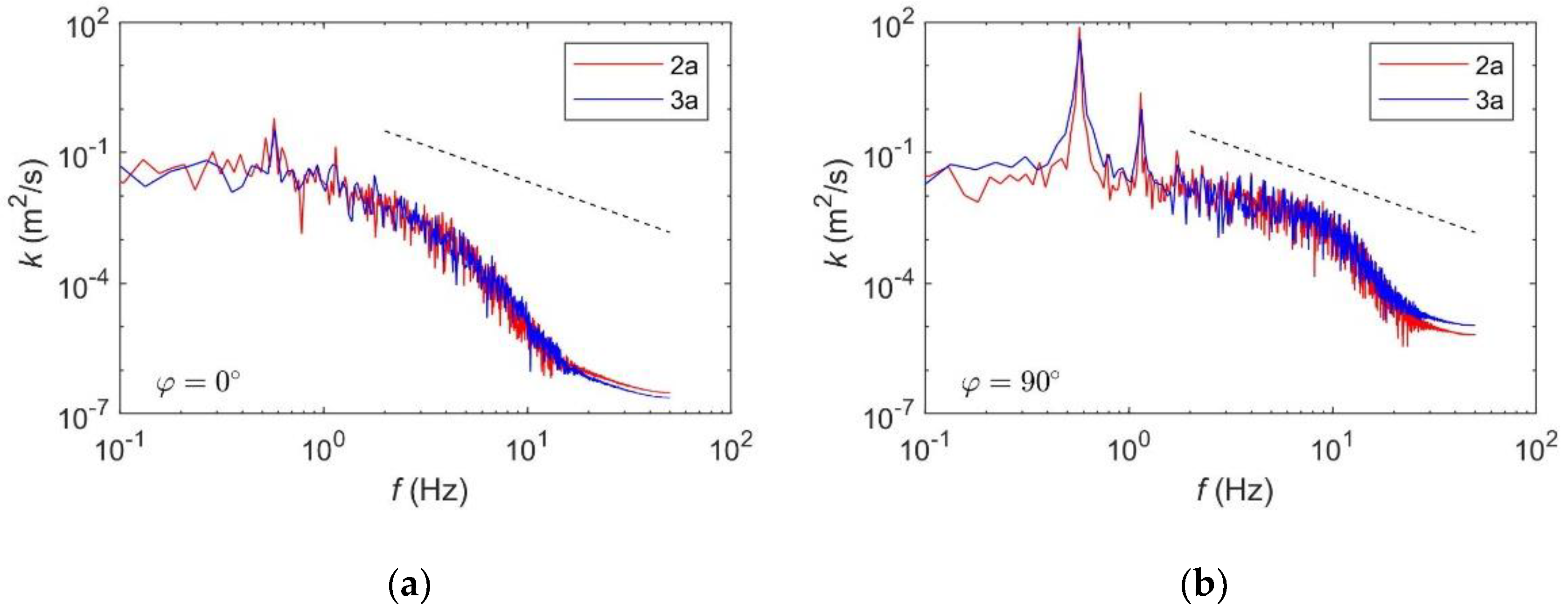
Figure 6 shows the spectra of the kinetic energy
K evaluated in the near-bed region (
z = 0.003 m) and around the cylinder at
φ = 0° (panel a) and
φ = 90° (panel b). A clear peak was observed corresponding to the frequency of the oscillating flow:
fp = 1/
T = 0.56 Hz. The frequency spectrum showed a decrease of the spectral energy content typical of turbulent fluctuations up to a frequency (
fu), where viscosity canceled out all the fluctuating motions. The developed range of scales was very tiny, being characterized by a few decades (the ratio
fu/fp was about equal to 30), suggesting that the turbulent flow emerging from the interaction of the oscillating flow with the vertical cylinder was very weak. Indeed, no evident inertial range, typical of fully developed turbulence where the spectrum was supposed to follow the
power law, was observed.
The above analysis of the fluctuating field had a strong consequence on the modelling approach. The observed weak behavior of turbulence challenged turbulence models, which are essentially conceived for fully developed turbulence. Furthermore, the simultaneous presence of laminar flow regions away from the pile and turbulence close to it, was again a challenge for turbulence closure, which should be able to recognize laminar oscillations induced by the wave motion where no model was needed from turbulence fluctuations where the model should be active. In conclusion, taking into account these turbulence modelling issues and by considering that the computational costs for a direct numerical simulation were relatively small due to the small separation of scales fu/fp, we argue that the DNS approach is strongly recommended for the solution of the wave action on a pile with no current.
In closing this section, let us further support the sensitivity analysis of the numerical approach reported in the previous section. Indeed, in
Figure 6 spectra are shown for both simulations 2a and 3a. The quality of the spectral convergence of results at different spatial resolutions is a clear indication of the accuracy of the numerical solution as already assessed in the previous section.
4. Results
In this section the results obtained in the two experimental campaigns and those of the numerical simulation are presented and compared. The validation was performed by the analysis of the main hydrodynamic characteristics, such as the water surface elevation, water particle velocity, pressure distributions and gradients, and total force over the pile. This section is finally closed by the analysis of the vortex pattern and of the related bed-shear stresses which are known to be the main cause of the scour formation. Performing direct experimental measurements of the shear stress was very complicated, hence, the use of a numerical simulation (fully validated) proved to be useful to get more information that can be very difficult to obtain in an experimental way.
The following subsections show the detail of the comparisons. In
Section 4.1 and
Section 4.2 are reported the comparison of the temporal evolution of the water level
η and the horizontal velocity
u. In
Section 4.3 and
Section 4.4, we make use of the so-called phase average of the analyzed data (pressure and force) in order to obtain values that express correctly the statistics at the wave phases of interest (
ωt). The phase average consisted of fixing the phase (
ωt) and averaging arithmetically all the “waves” of each realization. The reference wave phases
ωt were defined according to the water level evolution
η measured at elevation gauge S5, by assuming that
ωt = 0° corresponded to the up-crossing of the water level signal. Finally, in
Section 4.5 the results on the vortex pattern, the time-averaged streamlines, and shear stress linked with the equilibrium seabed morphology are reported.
4.1. Water Surface Elevation
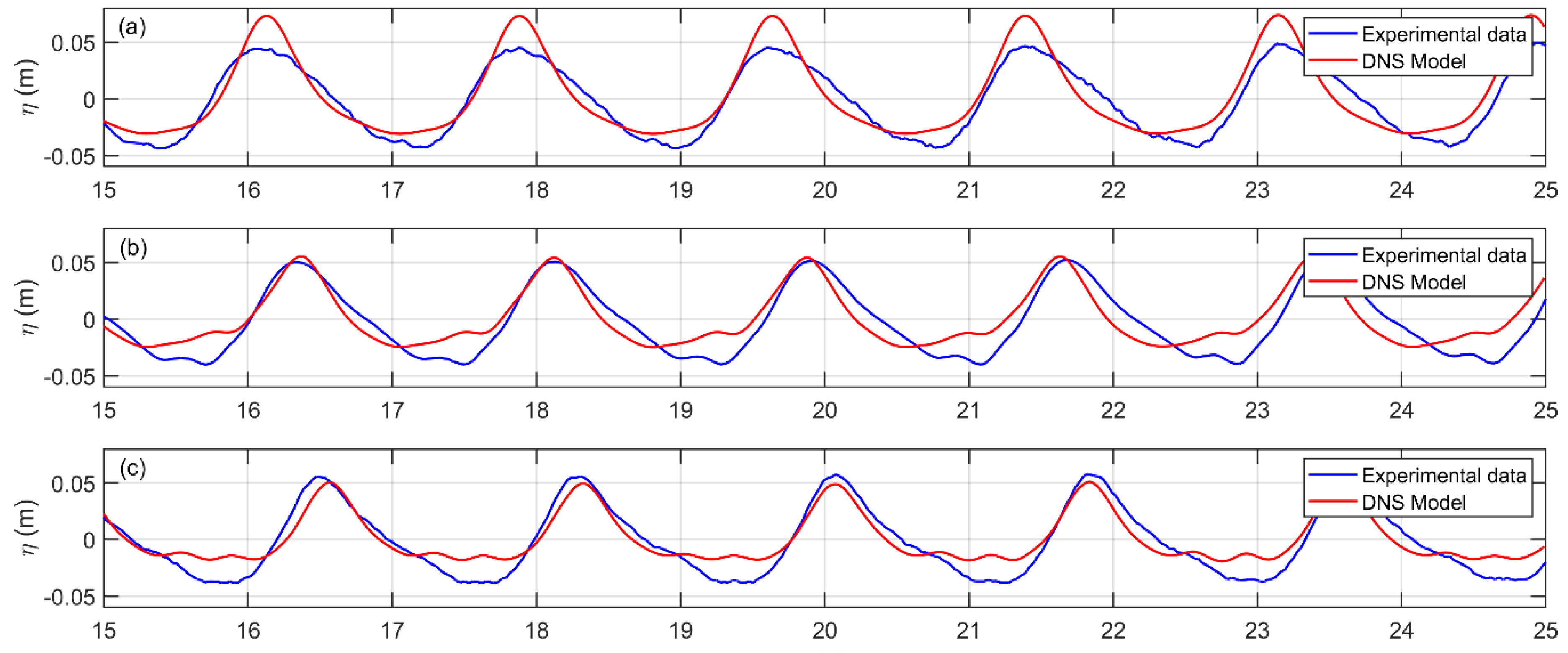
The comparison in terms of water surface elevation was realized in correspondence to the three water level gauges placed inside the numerical domain at the same relative distances from the pile of the water level gauges (S3, S4, and S5) of the experimental model. The results are shown in
Figure 7. Although the wave was run with the same characteristics at generation both in the experimental and in the numerical models, the wave generation and propagation processes in intermediate water depths led to nonlinear effects such as changes in the wave shape.
In the experimental model, the wave was generated at about 17 m from the pile, while in the numerical model at about 3 m. The nonlinear effects acted differently during the wave propagation over the flume, being more significant at the beginning of the wave propagation, closer to the wave generation. Therefore, such nonlinear effects were more evident in the numerical data (see
Figure 7) because of the relative smaller distances between the water level gauges (S3, S4, and S5) and the wave generation boundary. Such behavior explained the small discrepancy between the water surface elevations of the numerical and experimental models observed in
Figure 7. Even if a scatter was observed, the water elevation time evolution in correspondence to the pile (elevation gauge S5) showed a good agreement, especially for the evaluation of the maximum values of the wave crest. Even if the wave was rather nonlinear, due to the processes of generation and propagation along the flume in intermediate water depth condition, the nonlinearity of the water level elevation did not reflect to a high nonlinearity of the associated velocities [
12,
13], which can be well represented by the linear wave theory, as stated also by Le Méhauté [
14].
4.2. Particle Velocity
The reliability of the mesh quality of the model has been fully explained in
Section 3. The validation of the model was performed by, among the others, the analysis of the horizontal velocity of the water particles in specific points close to the cylinder (at
φ = 0°, 90°, and 180°, as shown in
Figure 2b).
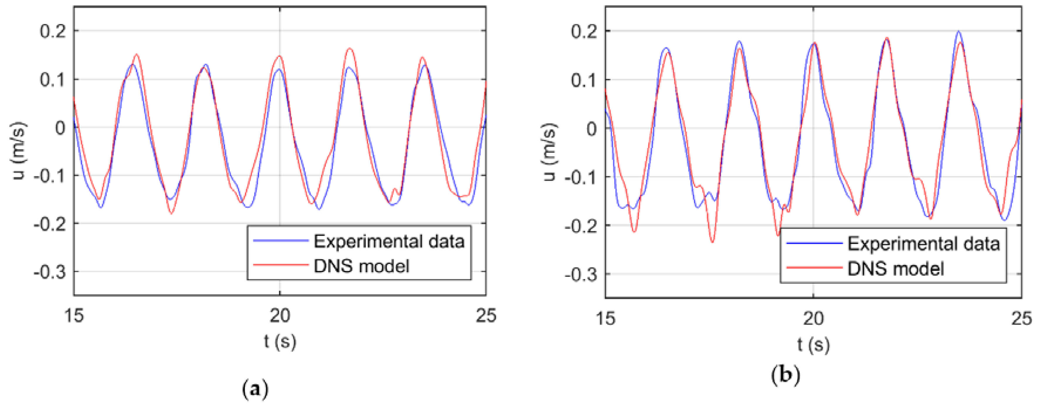
As an example, in
Figure 8 the comparison between the experimental (red line) and numerical data (blue line) yielded in front of the pile at different heights (
φ = 0°, z = 0.01–0.24 m) is reported. Even if the nonlinearity of the water surface was not reproduced in the same way (as showed in
Figure 7), the DNS model well represented the horizontal velocity magnitude and the shape of the velocity under the crest and trough phases, although the maximum values were slightly over estimated.
4.3. Pressure Distribution
In the present section the comparison of the vertical pressure distributions and the pressure gradients are analyzed. All the pressure P refers to the atmospheric pressure, hence it is null at the free water surface.
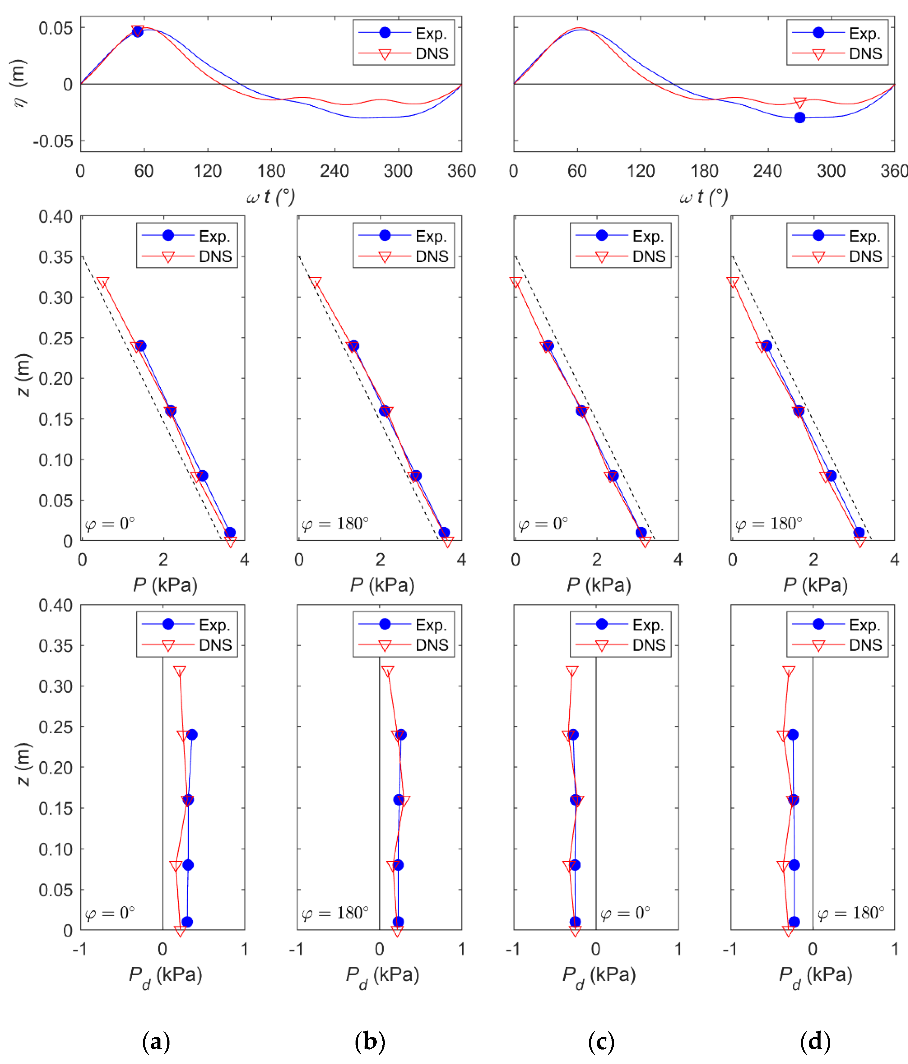
The experimental pressure distributions were compared with the numerical data. In
Figure 9, the comparison of the vertical distribution of the pressure
P evaluated in front of the pile (
φ = 0°) and behind it
(φ = 180°) is reported. By analyzing the pressure distributions for each wave phase, it was observed that the discrepancy was mainly due to the small difference in terms of water level elevation between the numerical and experimental data. The phase-averaged analysis of the water elevation
η revealed that the wave crest occurred at wave phases
ωt = 65° and
ωt = 63°, respectively, for the experimental and numerical models, while the down-crossing occurred at a larger wave phase for the experimental model with respect to the numerical one. Moreover, as argued in
Section 4.1, a lower wave trough and larger nonlinearities were observed in the numerical model. Despite the small difference in the water level elevation, the pressure results showed a quite good agreement. The lower panels of
Figure 9 show the vertical distributions of the dynamic pressure
Pd evaluated in front of the pile (
φ =0°) and behind it
(φ = 180°) for the wave phases
ωt = 45° and
ωt = 270°. The dynamic pressure
Pd is given by the difference between the pressure
P and the hydrostatic pressure
(
is the water density and
g the gravity acceleration). The analysis of the dynamic pressure distribution around the pile was very important because its asymmetry with respect to the vertical plane (
yz-plane) produced a horizontal force on the cylinder acting along the
x-axis. During the growth of the positive water surface elevation (e.g.,
ωt = 45°), a larger dynamic pressure
Pd was observed in front of the pile with respect to the area behind it; hence, a positive horizontal force was expected. During the negative water surface elevation (e.g.,
ωt = 270°) the pressure distributions in front of and behind the pile were quite similar; hence, the horizontal force along the
x-axis was expected to be very small (in absolute value). Moreover, the dynamic pressure data at
φ = 90° and
φ = 270°, here not shown, were similar, confirming that the horizontal force along the transversal direction
y was negligible, as found in
Section 4.4.
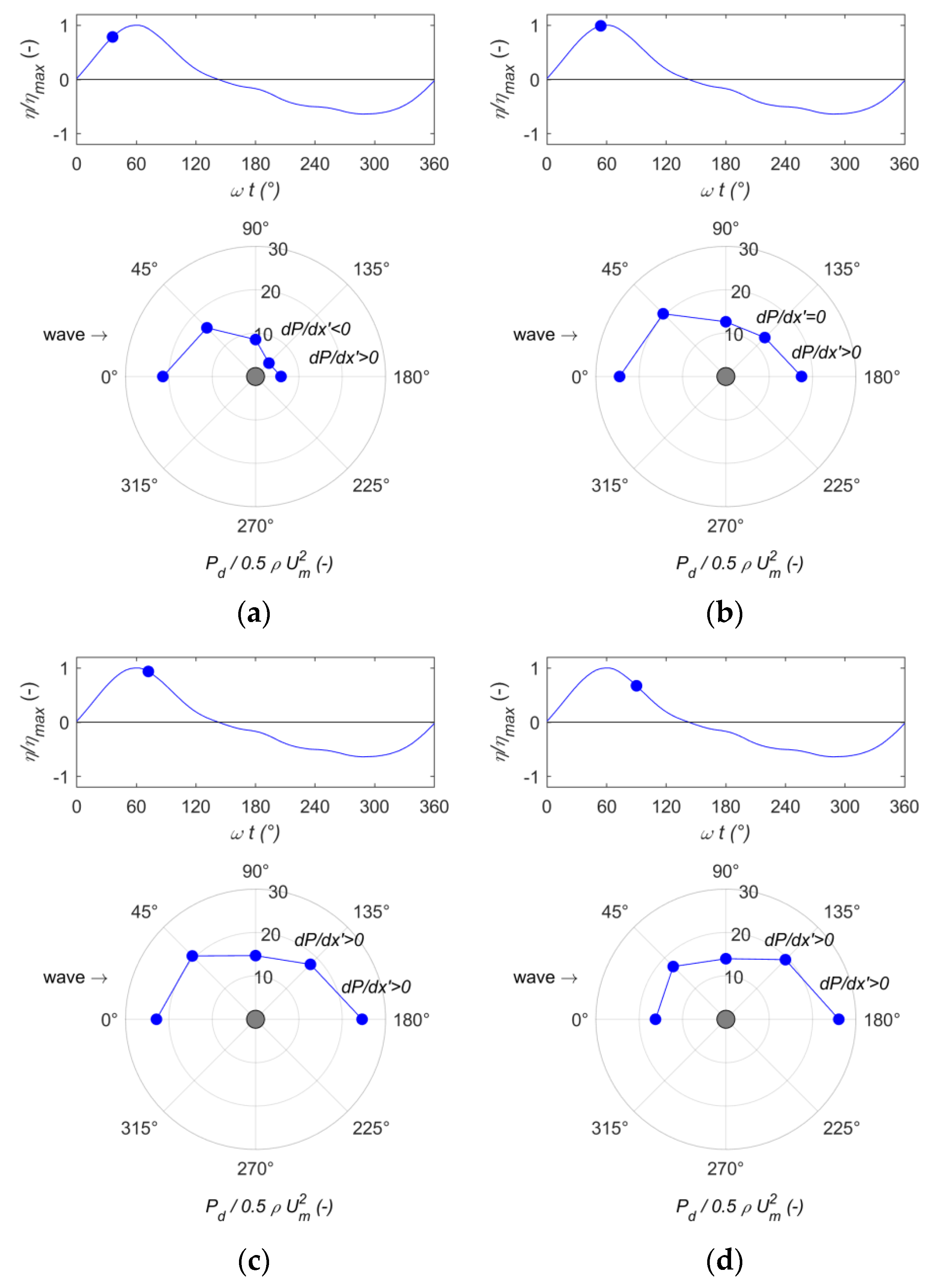
The measurements of the dynamic pressure around the pile also enabled us to confirm the presence, for specific wave phases, of positive pressure variations which induced the separation of the flow within the boundary layer and the subsequent formation of vortices. In
Figure 10, the plan view (
xy-plane) of the dynamic pressure distribution around the pile is shown at
z = 0.01 m. The pressure gradients around the pile
dP/dx’ (
dx’ is the length of the arc of the cylinder circumference formed by the angle
Δφ = 45°) were studied only experimentally, because the pressure sensors were located at
Δφ = 45°, while in the numerical model
Δφ was too large (
Δφ = 90°).
The dynamic pressure distribution was reported for specific wave phases: Two wave phases (
ωt = 36° and
ωt = 54°) representing the rising (
Figure 10a,b) and other two wave phases (
ωt = 72° and
ωt = 90°), representing the decaying of the positive water surface elevation (
Figure 10c,d). Only wave phases corresponding to the positive water surface elevation are shown, in order to emphasize the pressure variations and, hence, support the subsequent analysis of the physical process. The pressure distribution showed an asymmetric shape with respect to the
y-axis, which changed with the wave phases. During the rising of the positive water surface elevation, a favorable pressure gradient (
dP/dx’ < 0) was observed around the pile. Such condition was needed for the transport of the horseshoe vortices generated in front of the pile, as found during the mobile-bed experiments [
10,
15]. From the wave phase
ωt = 36°, the pressure gradient
dP/dx’ switched back to positive values (adverse pressure gradient) within a small area (
φ = 135°–180°). Such area became increasingly larger. After the occurrence of the wave crest, the adverse pressure gradient affected the area
φ = 90°–180°. Such conditions led to the separation of the flow within the boundary layer and, hence, to the formation of lee-wake vortices, which were the main properties responsible for the scour under the wave action. Such findings were in agreement with the results of the vortex pattern reported in
Section 4.5, confirming that, for specific wave phases, the coherent structures were formed, developed, and transported during the interaction of the flow with the cylinder.
4.4. Total Force
In this section the total horizontal force acting over the surface of the pile is analyzed. The forces acting on slender cylinders were often evaluated by the Morison equation [
1] for linear small amplitude waves. Here, Equation (2), the total wave force is computed as the sum of two different components, a drag force (
FD), and an inertial component (
FI).
where
CD and
CM are, respectively, the drag and inertia coefficients.
The drag force, which depends on the square of the velocity, is given by the asymmetric pressure distribution around the pile. Indeed, in the wake zone, the pressure tended to a constant lower value. The cylinder geometry dove the fluid to go around it, modifying all the local particle velocities and accelerations, thus originating the inertia force. This equation proved to be a good approximation for the estimation of the force, although it has some weak points. Indeed, the integration was done considering the linear superposition of the two components which reached the maximum values at different wave phases. The wave was considered linear, and the run-up and the impact force were not considered. Furthermore, the estimation depended on two experimental coefficients, which vary with the geometry, the roughness, and the characteristics of the flow and, for simplicity, were considered constant along the pile and for all the wave phases even if they varied in an oscillatory flow because of their dependence on the flow. In the DNS model, the total force acting over the cylinder was computed at every time step as the integration of the pressure of the wet points over the whole surface.
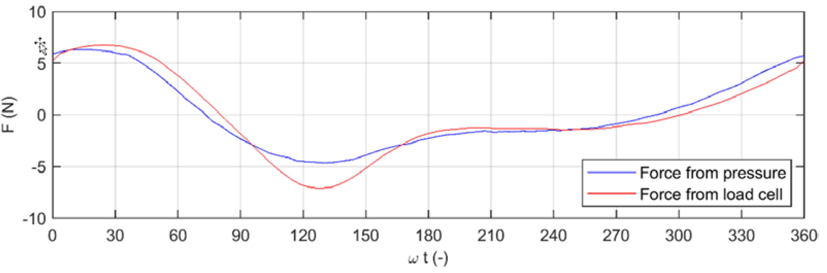
The pile of the experimental model was equipped with a hinge at the bottom and it was fixed with the load cell on the other end at the upper side. According to this setup, the measured horizontal force at the load cell was elaborated to obtain the wave force over the pile that depended on the lever arm between the line of application of the force and the hinge (bW). Knowing the distance between the load cell and the hinge (bC = 1.04 m) and estimating for each time the distance bW, the force on the pile was obtained. These assumptions were verified by means of a calibration process of the load cell, applying different known horizontal forces at different locations.
The force obtained by means of the load cell measurements was compared with that obtained by means of the integration of the pressure distribution recorded around the pile (
Figure 11). The results show a very good agreement between the two sets of data, especially during the crest phase. The underestimation of the minimum value of the force can be due to the discretization of the pressure distribution around the pile. Therefore, although the pressure sensor discretization was not tiny (
Δφ = 45°,
dz ≈ 8 cm), the comparison of the force obtained by two different types of measurements confirmed the validity of the data.
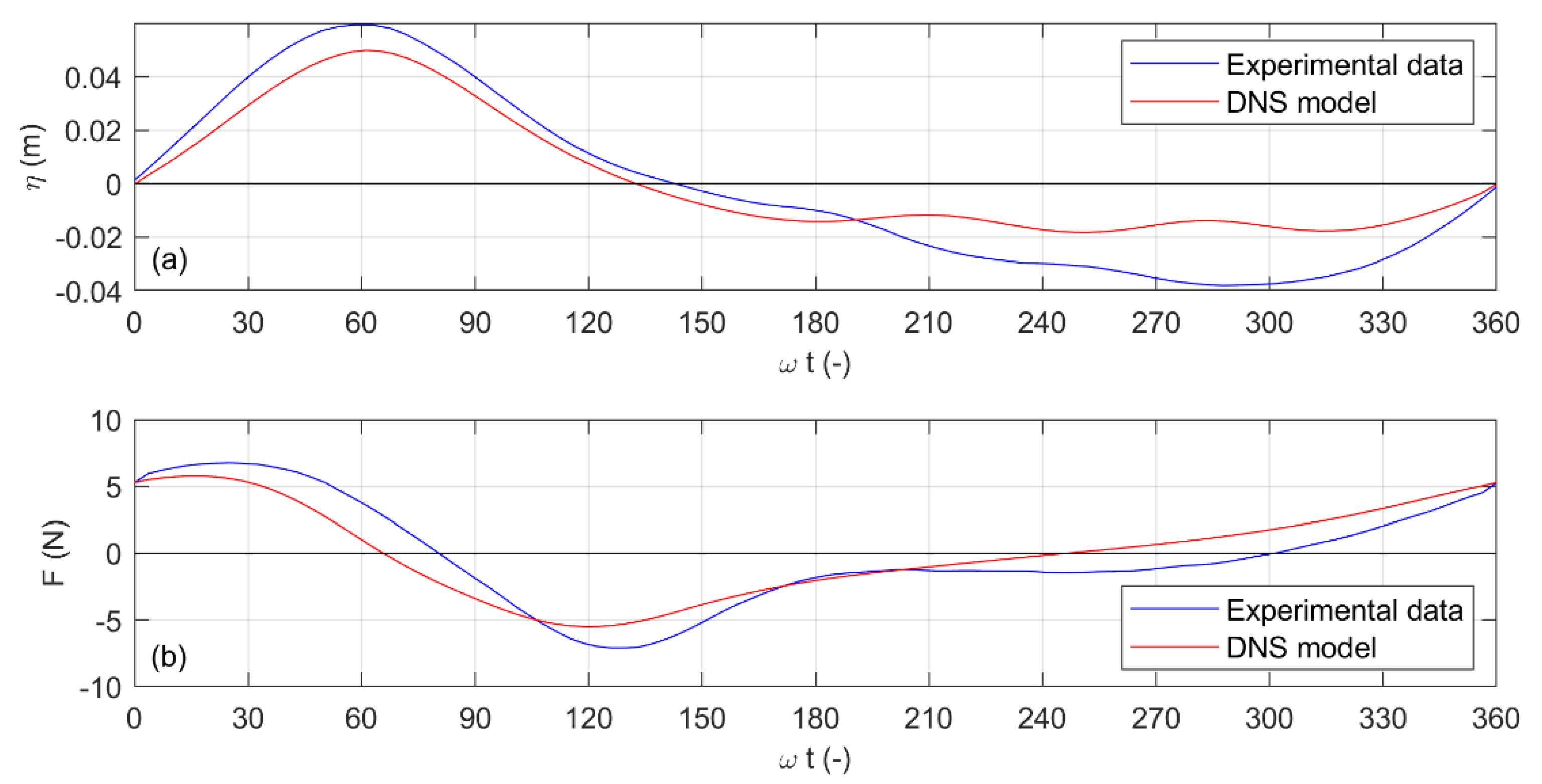
Figure 12 and
Figure 13 show the phase-averaged force, along the
x direction, evaluated both numerically and experimentally. The wave forces along the transversal direction (
y-axis) were found to be negligible.
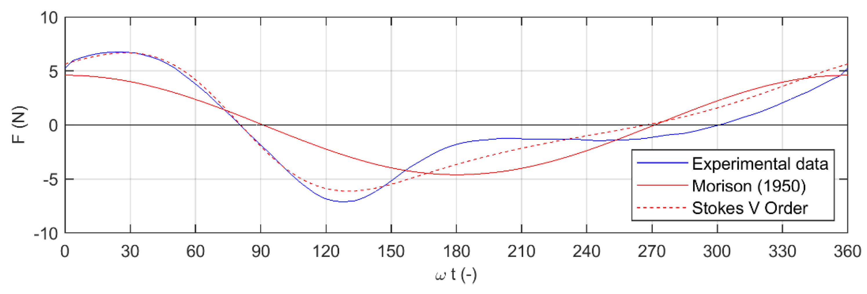
Although the shape of the wave of the numerical model is steeper and reveals a larger nonlinearity than that of the experimental test, a very good agreement over the evaluation of the force was achieved. The maximum numerical value was slightly lower, according to the lower wave crest elevation. The shape of the force evolution along the wave phases was very similar; the slight shift of the force signals was only due to the difference in the occurrence of the wave crest between the numerical and experimental data, as already pointed out in
Section 4.3. Therefore, the dynamic response of the wave over the cylinder was well reproduced and the model can be considered fully validated.
The theoretical evaluation of the wave force over a vertical cylinder can be made by using Equation (2). The problems of its application for design purposes are the correct evaluation of the water particle velocities and accelerations and the choice of the right drag and inertia coefficients (usually obtained for smaller Reynolds numbers with respect to prototype conditions [
16,
17]). The direct integration can be performed with the hypothesis that the coefficients are constant, the wave is linear (Airy’s theory), and its amplitude can be considered small in comparison with the water depth (Morison formula [
1]). These assumptions cannot be considered reliable for real water waves, which show nonlinearities, with a more peaked wave crest and a more flattened trough.
Furthermore, the right choice of the coefficients of Equation (2) plays a significant role on the evaluation of the force acting on the pile. For the present laboratory conditions, according to the work of Sarpkaya [
16], a pair of drag and inertia coefficients are chosen (
CD = 0.9 and
CM = 2.0). The application of the linear theory as for the evaluation of particle velocities and accelerations could lead to a significant underestimation of the maximum value of the force (here about –30%). The use of higher order theories in Equation (2) (e.g., Stokes V order theory) improved significantly the estimation of the maximum value of the wave force, as shown in
Figure 12, and allowed us to better reproduce its trend over the whole wave period (the velocities and the accelerations of water particles were computed according to the methodology proposed by Fenton [
18]). Therefore, the use of the Morison equation with higher order wave theories is recommended for the prediction of the wave force on the pile.
4.5. Flow Pattern, Shear Stress, and Scour
In this section we make use of the different information provided by the numerical and experimental approach in order to highlight the relevant physical processes responsible for the scour at the base of the pile, which would be otherwise difficult to understand by solely using experimental or numerical data.
It is well known that the process of scour in the wave regime significantly depends on the wave characteristics and, hence, by the Keulegan–Carpenter number. As shown by Corvaro et al. [
10], the formation of the scour is mainly due to the presence of phenomenon of shedding of vortices at the base of the pile. Accordingly, we made use of the direct numerical simulation data to analyze the flow pattern around the pile. More in detail, we made use of the second invariant Q of the velocity gradient tensor
(the velocity gradient
can be decomposed into a symmetric and a skew-symmetric part
where
is known as the rate-of-strain tensor and
as the vorticity tensor), defined as:
Indeed, it is well known that connected flow regions characterized by a positive value of the second invariant,
Q > 0, allow the identification of vortical structures [
19].
Q represents the local balance between shear-strain rate and vorticity magnitude, defining vortices as areas where the vorticity magnitude is greater than the magnitude of rate-of-strain [
19,
20]. In
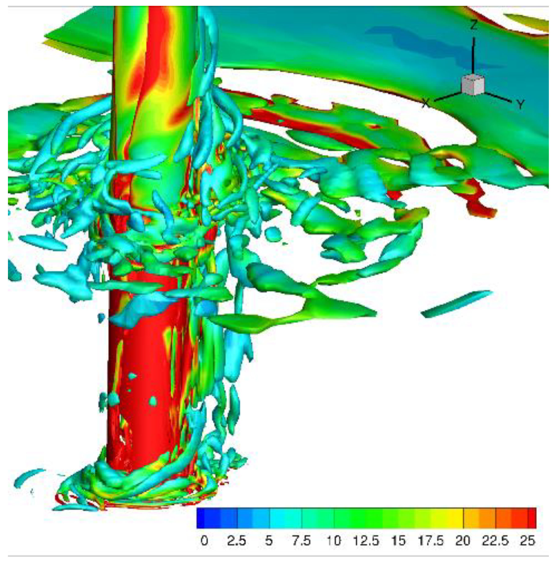
Figure 14, the isosurface
Q = 10 colored by enstrophy (the square of the vorticity vector) is shown.
As can be seen, the wave motion and, consequently, the alternating flows gave rise to a complex flow pattern consisting of shedding of structures from the pile. In particular, vortices were found to be essentially aligned in the vertical direction along the pile, while, at its base, flow motion organized in structures that lie in the horizontal direction forming ring shapes around the vertical cylinder. The vertical-aligned and ring-like vortex structures of the flow are known to play an important role on the fluid dynamic loads on the vertical cylinder and on the erosion phenomena at its base. These two flow structures are commonly referred as lee-wake and horseshoe vortices, respectively, see Sumer et al. [
5].
As extensively argued by Sumer et al. [
5], one of the process related to the vortex formation is an increase of the bed-shear stress which, in turn, is related to the scour process. Again, here we made use of the combined information from the numerical and experimental models to shed light on this phenomenon. The vortex-flow regimes, the bed-shear stress, and the scour are all related together and governed primarily by
KC [
4,
5].
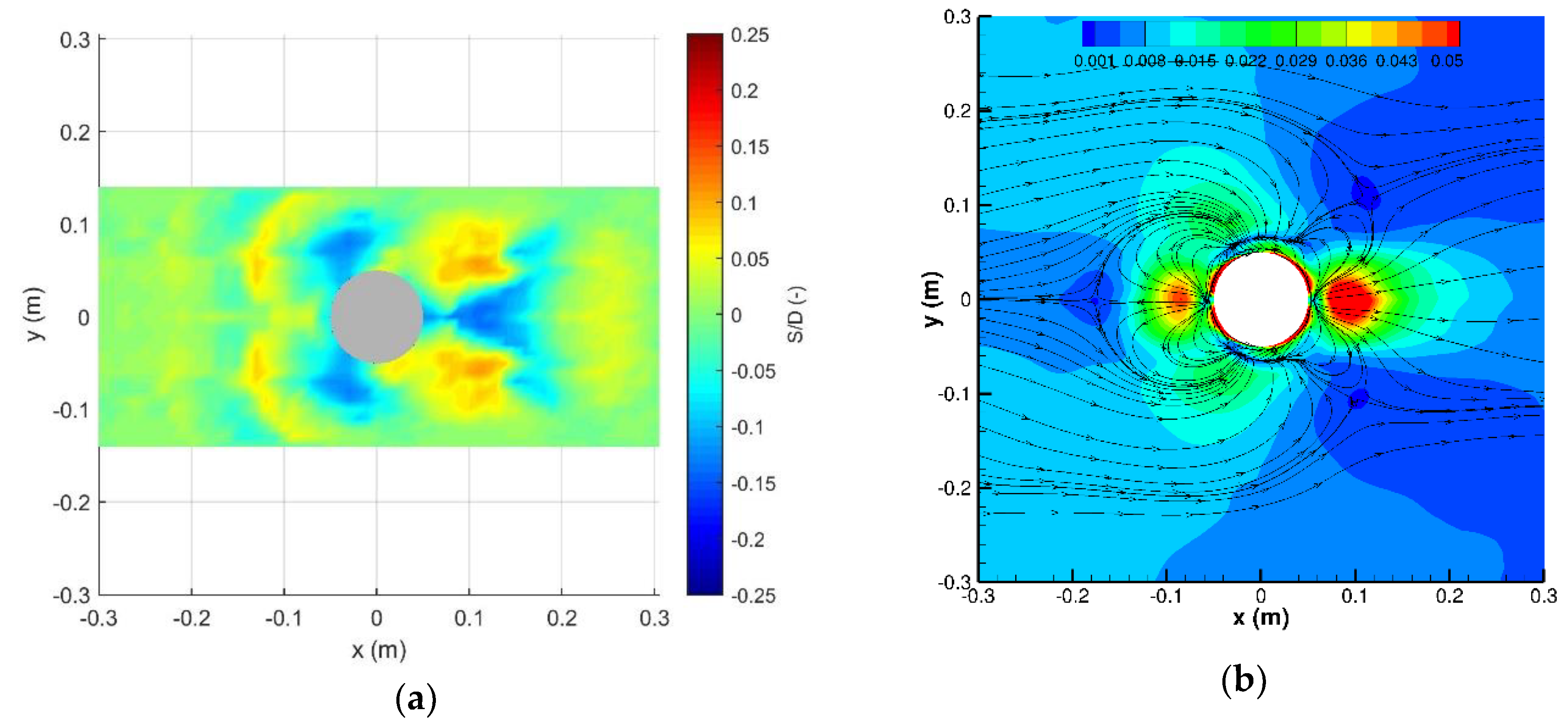
Figure 15 shows the measured scour pattern obtained in a previous experimental campaign with a mobile bed (Corvaro et al. [
10]) for a wave characterized by a value of
KC similar to that of the wave here analyzed. In particular,
Figure 15 plots the nondimensional scour
S/D, where
S is the scour depth and
D is the pile diameter. The analysis of the seabed morphology revealed that the area subjected to the maximum scour was located behind the pile (φ = 180°) at a distance of about 10 cm (1.0
D) and the maximum value of
S was equal to 1.4 cm (
S/D = 0.14). The most widely used formula for the scour prediction under regular waves is given by Sumer et al. [
4]. Other zones where scour occurred were located at
φ = ±45°, while deposit zones were observed at
φ = ±135° and in front of the pile (
φ = 0°).
In
Figure 15b, the computed bed-shear stress from the numerical simulation is reported. Note that an increase in terms of bed-shear stress and, thus, of turbulence levels, resulted in a tremendous increase in the sediment transport leading to the formation of a scour hole around the pile in a fairly short period of time [
21].
The comparison of the two plots proves that zones of high scour are associated with those of intense shear stress. However, the intensity of the shear stress alone does not allow us to distinguish zones of sediment deposition from those where erosion occurs. To overcome this limitation, in
Figure 15b the streamlines of the bed-shear stress vector field (
μ∂u/∂z, μ∂v/∂z) are also shown. The presence of the pile was found to strongly modify the shear-stress pattern that in free conditions would lead to a transport of sediment in the direction of propagation of the waves. Particularly, we observed four singularity points for the field lines. The first one is right in front of the pile and represents the origin of shear stresses transporting sediment in the upstream direction before symmetrically bending in the lateral directions. This lateral bending was induced by the interaction with the shear-stress field lines emerging further upstream and transporting sediment in the wave direction. This interaction gave rise to the second singularity point at (
x,y) = (−0.17 m, 0.00 m) and to two lateral arcs of convergence of the field lines. Hence, sediment was transported from the front of the pile towards the second singularity point and towards the two lateral arcs. In accordance with this picture,
Figure 15a shows a deposition of sediments conforming with these two paths and an erosion in the embedded region.
The third singularity point for the shear-stress field lines was located right in the back of the pile. From this point, two branches of field lines emerged. A central portion of the field lines transporting sediment was directed downstream. Hence, the rear central region of the pile was characterized by shear stresses whose action was solely of extracting sediment and transporting it downstream. Accordingly, the measured scour in
Figure 15a highlights the presence of erosion. On the other hand, the other portion of field lines was found to symmetrically bend in the lateral directions first and then to rise in the upstream direction. By moving upstream, the field lines interacted with those emerging from the upstream regions. The region of convergence of these two branches of field lines became thinner and thinner by moving further upstream and formed an arch shape which was finally closed by the last (fourth) singularity point where all these field lines converged. Overall, this pattern conformed with two lateral symmetrical regions of convergence of field lines transporting sediment from the rear of the pile and from the upstream regions whose size reduced by moving upstream, thus forming an arc shape. In accordance with this picture, the measured scour in
Figure 15a shows two symmetrical regions of deposition which became thinner by moving in the upstream direction. Finally, very strong shear stresses were found around the pile in proximity of it, confirming that in such area the bed forms typical of a mobile bed were destroyed.
5. Discussion and Conclusions
The combined use of direct numerical simulation and experimental data proved to be fundamental for a deep understanding of the hydrodynamics around a vertical cylinder under wave action. The convergence of the numerical simulation with experiments was achieved and its validation was performed by means of all the major hydrodynamic quantities. A very good agreement was found by the comparison of the water surface elevation, the water particle horizontal velocity, the pressure distribution around the pile, and the total wave force. The combination between experimental and numerical data is always the best procedure to guarantee the reliability of the results. Furthermore, once the numerical simulation was fully validated, it was possible to extract a huge amount of information that it is very difficult to obtain experimentally.
The analysis of the pressure distribution at different wave phases confirmed the presence of pressure gradients around the pile responsible for the formation, development, or transport of vortices. The asymmetric pressure distribution between the front and the wake region of the pile also produced a total force on it. The maximum force occurred during the rising of the positive water elevation (
ωt > 0°) and before the wave crest phase (
ωt ≈ 65°). Such result suggests that both the drag and inertial components of the total force are important. It is well known that the total force is maximum at
ωt = 0° when the inertial force is dominant, while it is maximum at the crest wave phase when the drag force is dominant. The application of the Morison’s equation [
1] to estimate the maximum force can lead to a significant difference with the experimental results for nonlinear waves. The problem of using this equation is on the assumptions made to simplify the calculations (linear theory, constant coefficients, small amplitude wave). Furthermore, the use of empirical coefficients is needed for its application and their determination from literature (e.g., [
16]) as a function of
KC and
Re is not easy. Several authors ([
22,
23]) addressed how the determination of the drag and inertia coefficients is not unique and depends on, among the others, the technique used for their estimation. As shown in
Figure 13, the simple application of the formula can lead to an underestimation of the maximum values of the force for the analyzed values of
Re (
Re ≈ 10
4). The use of the Morison’s equation with higher order wave theories improved the prediction of the maximum force and, hence, is recommended. Field conditions were associated with higher values of
Re (
Re ≈ 10
6 ÷ 10
7) and, thus, to correctly design a structure, a safety factor for the total force of 1.5 ÷ 2.0 was needed, due to the uncertainties on the determination of the coefficients in such conditions. Full scale experiments at higher Reynolds numbers were useful to optimize the design process.
The DNS model was able to reproduce correctly the main hydrodynamic characteristics. The analysis of the bottom shear stress gave useful information to understand the scour process. The wake region where the maximum shear stress was obtained corresponded with that of maximum scour for a wave with similar characteristics. The main deposit regions were located at
φ ≈ 150° (according to
Figure 2) and about 1.5 D from the axis of the pile. Such results were in agreement with the contour map of
Figure 15. Indeed, even if mobile-bed conditions can modify the bottom shear stress, the DNS model results of a rigid bed proved to be consistent with the seabed morphology data, providing qualitative information about the regions in which the bottom shear stresses are more significant. Furthermore, the analysis of the streamlines allowed us to understand the general movement of the sand around the pile and to explain the relation between the erosion and deposition zones. The formation of vortices, in addition to the streamline contraction, removed the sand particles from the surroundings of the pile, especially in the zone where the lee-wake vortices were stronger and, thus, the suspended particles tended to accumulate in the regions where the shear stress decreased.
Finally, by means of a spectral analysis of kinetic energy, it was pointed out that the wave action on a pile was responsible for an oscillating flow whose turbulence fluctuations were weak and confined in the pile region. These aspects challenged for turbulence closures that should be able to distinguish laminar oscillations induced by the wave motion from turbulence fluctuations. Given these modelling issues and by considering the relatively small computational costs of a DNS due to the small separation of scales generated by the wave action on a pile without current, we finally strongly recommend the use of a DNS approach for the solution of these types of problems.


