Transitional Flow on Model Propellers and Their Influence on Relative Rotative Efficiency

Abstract

Unexpected low value of the relative rotative efficiency η_R is sometimes noted when scaling the towing tank model-test result with the ITTC-78 method to obtain the propulsive efficiency factors of propellers. The paper explains the causes of this phenomenon. The boundary layer state of three propellers was studied by a paint test and a RANS method. The paint tests showed that the propellers in behind conditions at low Reynolds number (Rn) are covered mainly with laminar flow, which is different from open water tests conducted at a high Rn. Apart from that a moderate difference in Rn between the open water and the self-propulsion test may lead to a low η_R value, the paper points out that flow separation in behind conditions could be another significant reason for the drop of η_R for some propellers. Therefore, two factors will lead to an unexpected decrease of η_R: (1) A slightly lower open water torque interpolated from an open water test carried out at a high Rn and (2) a slightly higher torque in a self-propulsion test due to laminar flow separation near the trailing edge. The phenomenon is caused by the Rn scaled effect and closely associated with design philosophy like the blade section profile, the chord length, and chordwise load distribution.

1. Introduction

In 1978 the International Towing Tank Conference (ITTC) published its recommended power performance prediction method, known as ITTC-78 method, to scale the towing tank model-test results to full-scale ship performance. This method has been used for four decades. The method works well in most cases. However, when applied for propellers designed with non-conventional design philosophies, e.g., propeller with extremely low blade area ratios, unusual radial and chord wise load distributions, unusual sectional shapes, and tip fins of various types, the scaling method encounters new challenges on the Reynolds number (Rn) scaling procedure. Throughout the paper, the Rn number is based on the chord length and the resultant velocity of the blade section at 0.75R radius, with R being the propeller radius. The paper pays special attention to the low blade area propellers, where a drop of the relative rotative efficiency η_R is sometimes encountered when using the ITTC-78 method. If the drop of η_R is not physical but due to a too simple Rn-scaling scheme, it will lead to an unfavourable full-scale performance prediction. A number of investigators, for example, Tamura and Sasajima [1], Tsuda et al. [2], and Hasuike et al. [3,4,5] attributed this phenomenon to an Rn number difference (i.e., Reynolds scale effects) between the propeller open water test (POT) and the self-propulsion test (SPT) that causes a difference in the boundary layer flow between the two tests. Due to the low operational speed of the model ship and the propeller during an SPT test (as required by Froude’s scaling law), the Rn number in an SPT is lower than that in a POT. When determining the relative rotative efficiency η_R, an open water torque coefficient K_Q0 needs to be extracted from the open water (POW) characteristic curves obtained from a POT. If the POT is carried out at a high Rn as proposed in the ITTC-78 method, the extracted K_Q0 may not be fully representative of the propeller characteristics at the low Rn as used in the SPT. For this reason, an alternative scaling method, called “2POT method,” was proposed and used by a few ITTC member organizations. It consists of performing two sets of POTs, one at a low Rn equal to the Rn in an SPT test and the other POT at a sufficiently high Rn. The low Rn POW data is used to analyse the SPT results (i.e., determining wake fraction w_Tm and relative rotative efficiency η_R etc.) whereas the high Rn POW is used to scale the POW to full scale. The rest of the scaling procedure for powering prediction in the 2POT method is the same as the ITTC-78 method.

Apart from the 2POT method, there are other scaling methods that have been developed and are being tested to account for scale effects of propellers especially those of unconventional design. For example, the “Strip Method” by Streckwall et al. [6], in which a local skin friction coefficient is used to compute the sectional drag by integrating the laminar and the turbulent part of skin friction contribution. For this purpose, two friction lines were developed for each blade section, with one line applicable in the POT condition and the other applicable in the SPT condition. Helma [7] presented an extrapolation method suitable for scaling the POW of various propellers. Lücke and Streckwall [8] applied the paint test on three model propellers in behind and open water conditions to visualise the boundary layer flow structure on blades. The scaling issue and propulsion performance method were discussed accordingly. They found a high amount of laminar flow on all propellers in POT and SPT conditions at a Rn number corresponding to the SPT condition. They also noted the streamlined orientation in the SPT condition has a more gradual change in contrast to a sharp separation zone in the POT condition. Heinke et al. [9] applied an interpolation scaling procedure based on a set of POT tests carried out at multiple Reynolds numbers. Analyses of Rn scale effects and scaling methods for ducted propellers and non-conventional propellers have been addressed by Bhattacharyya1 et al. [10,11,12], Sánchez-Caja et al. [13], Shin and Andersen [14], and Moran-Guerrero et al. [15] recently.

With regard to CFD RANS methods for analysis of transitional flow around propellers, the most relevant work is due to Hasuike et al. [3,4,5], where the authors applied a laminar-kinetic-energy based k-kl-ω model to determine the laminar flow on many low blade area propellers and compared it with available experimental data. The results demonstrated the presence of a large amount of laminar flow on blades in open water and behind conditions when the propeller is operated at low Rn numbers. Baltazar et al. [16] employed a γ-Re_θ transition model to predict POW performance of a conventional and a high-skew propeller in model scale and compared the results with the model test and an SST k-ω model. Improvement on transition model in itself is still an ongoing research, as discussed, e.g., in papers by Gaggero and Villa [17], Colonia et al. [18], Lopes et al. [19] and Moran-Guerrero et al. [20].

In the standard ITTC-78 method, the POT shall be carried out at a sufficiently high Rn and the Rn should, in any case, be greater than the critical Reynolds number Rnc (normally considered to be Rnc ≈ 3 × 10⁵). During a self-propulsion test where Froude scaling must be applied, the ship and the propeller model are operated at rather low speeds. Typically, the Rn based on sectional chord length at nominal radius 0.75R (R is the propeller radius) is limited to a range of 1~3 x10⁵. Clearly, there is a difference in Rn between the POT and the SPT, yet the difference is moderate, and the two Rn numbers are within the same order of magnitude (10⁵). This difference is much smaller than the Rn difference between a model scale (10⁵) and a full-scale propeller (10⁷). One question is how much the Rn scale effect will be introduced with this moderate difference for model scale propellers. Would different propellers react to this Rn difference differently? Operating a propeller at a Rn number lower than Rnc would imply the occurrence of laminar flow and possibly flow separation. On the other hand, for a propeller in the behind condition, the elevated turbulence intensity in the wake of the ship model would make the propeller more susceptible to turbulence transition. One would wonder how large a blade area is covered by laminar flow in an SPT. What is the difference in the boundary layer characteristics for a propeller in the behind condition and in the open water condition at the same Rn? What is the reason for the unexpected low η_R value and what type of propellers have such an issue?

The aim of the present work is to address the above five questions by means of model testing, combined with a RANS method coupled with a transition model. It investigated the boundary layer flow over the blades of three model propellers. The chosen propellers represent a low blade-area high-efficiency propeller (of NAKASHIMA design), and two conventional designs with a medium and a high blade area, respectively. The POT test and paint test were conducted for these propellers at a low and a high Rn number. The paint test was also performed in the behind condition to look at the difference in the near wall boundary layer flow. For the RANS method, the Menter’s SST k-ω turbulence model [21] coupled with the turbulence intermittency transition model by Menter et al. [22] was used. The model is called the γ-model. The bypass transition and separated-flow transition are the most dominant transition phenomena occurring on model scale propellers. They are triggered by a variety of possible flow disturbances such as free-stream turbulence, pressure gradient, wall roughness, flow instabilities in the form of elongated streamwise streaks, and intermittent turbulent spots. For rotating bodies like the propeller, cross flow instability plays an important role in the transition onset. Since the γ-model [22] includes a term to account for the cross flow effect, it is considered appropriate for the present study.

2. Propeller Model and Model Tests

The main particulars of propellers are presented in

Table 1. Main particulars of the propellers.

Propeller	AE/A0/Z	P/D0.75R	tmax/C0.75R	C0.75R/D	Number of Blades
Prop A	0.10	-	-	-	-
Prop B	0.13	0.83	0.0350	0.27	4
Prop C	0.16	1.00	0.0438	0.33	5

, in which D is the propeller diameter and R is the radius. The t_max/C_0.75R is the maximum thickness-to-chord ratio at the 0.75R blade section. For confidentiality reason, some data for Prop A is not shown in the table.

In a POT, the propeller model was mounted on a horizontal shaft and towed through the water at an immersion depth of the shaft center equal to one propeller diameter. During the test, the rate of revolutions was kept constant while the advanced speed was varied to achieve a series of advance ratios (J). In SPT tests, the same hull model was used for the propellers. Prop A was designed for this hull form. Therefore, the SPT for Prop A was performed at design speed whereas the SPT for the other two propellers was performed at an off-design point.

The paint test is used to detect the boundary layer state of the flow over blades. Before the test, the propellers were painted with a black paint along the leading edge (LE). During the test, the flow direction of paint is governed by the skin frictional force and affected by the inertia. For a blade area covered with laminar flow where the skin frictional force is not strong enough to make the paint following the circular movement on the blade, the inertia (apparent centrifugal force) of the paint makes it move in the outward radial direction. Therefore, the traces of the paint will mainly follow the radial direction. For a blade area covered with fully turbulent flow where the shear stress force is large enough to hold the paint along the circumferential direction, the paint traces will look more like circular lines. In the paint test, the propeller was mounted in the same way as in POT and SPT, but only one run at one speed was made each time. The test was performed at a high and a low Rn number for each propeller according to the loading conditions defined in

Table 2. Loading conditions for POT.

	Prop A		Prop B		Prop C
Condition	Low Rn	High Rn	Low Rn	High Rn	Low Rn	High Rn
N [rps]	8.1	20	6	18	5	15
VA [m/s]	1.214	3	1	3	1	3
J [-]	0.646	0.646	0.694	0.694	0.824	0.824
Rn [x105]	2.06	5.08	2.15	6.46	2.24	6.71

. Photographs were taken after each test. The chosen low Rn numbers corresponded to a typical Rn used in an SPT.

3. Numerical Methods

3.1. Numerical Models

The viscous flow is solved by an incompressible Reynolds Averaged Navier-Stokes (RANS) method using ANSYS FLUENT 18.2. The Menter’s Shear Stress Transport (SST in short) k-ω turbulence model [21] is employed for simulation of the propeller in a fully turbulent flow. The result serves as a reference for comparison with the transition model.

To simulate the laminar flow and transition to turbulence flow, Menter et al.’s intermittency transition model [22] is employed. The fraction of the time during which the flow over any point on the surface is turbulent is defined as “turbulence intermittency.” This transition model, denoted as the γ-model, is a further development of the γ-Re_θ model based on the coupling of the SST model with a transport equation for the intermittency γ. It inherits the same underlying modelling concept as the γ-Re_θ model, e.g., local-correlation based transition modelling, and the correlation between transition phenomena and free stream turbulence intensity and pressure gradient. The detail is referred to in Reference [22]. The model has an option important for cross flow transition, which is used in the present work.

3.2. Numerical Schemes

The following schemes are used:

• Incompressible pressure-based solver.
• Pressure and velocity solved in a coupled manner.
• Second order discretisation for pressure gradient at face.
• QUICK scheme for all transport equations.
• Single Reference Frame for POT calculation in a steady mode.
• Sliding mesh grid interface for calculation in the behind condition in an unsteady mode.

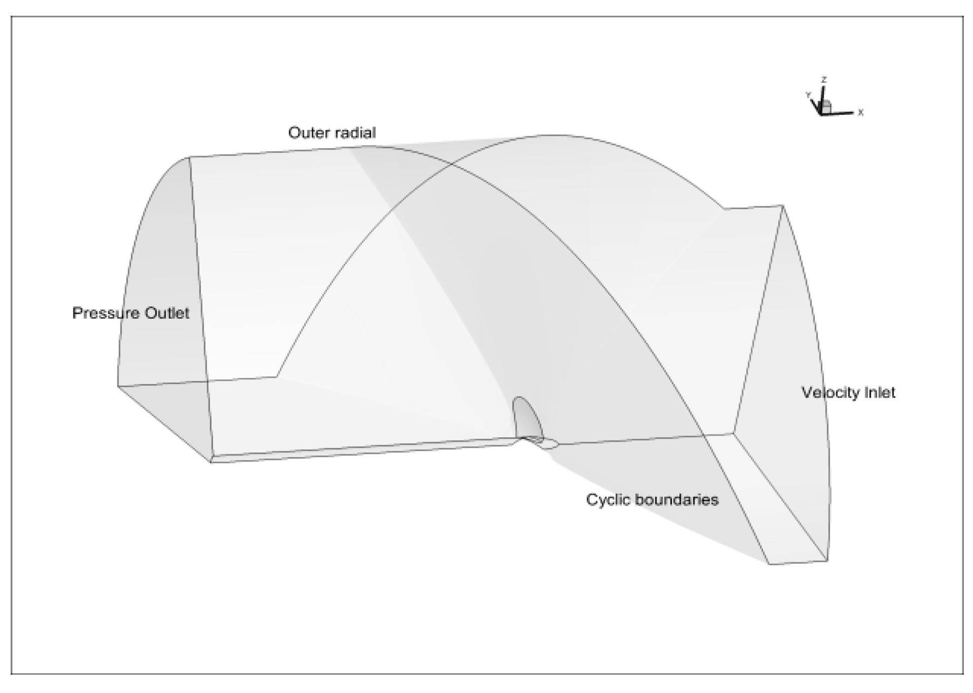
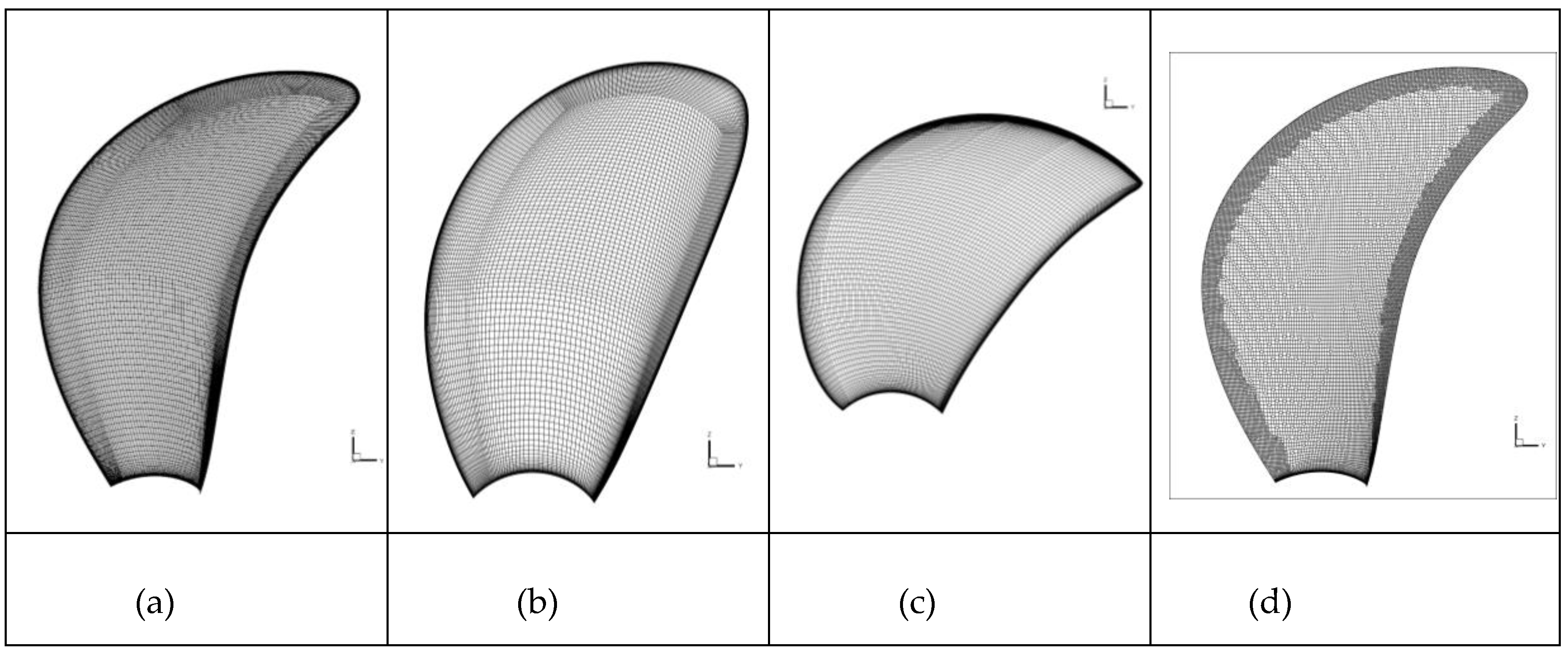
3.3. Computational Domain and Mesh

For simulation in the POT condition, the CFD domain consists of a blade passage by utilizing the circumferential periodic boundary condition (BC) and single rotational reference frame (SRF). The distance of the domain boundaries to the center of the propeller are defined as a multiple of propeller diameter D. Namely, Inlet = 2D, Outlet = 3D, and Outer radial = 3D. The meshes generated on the two periodic surfaces are fully conformal. All meshes are of hexahedral type and generated by ICEMCFD Hexa. The non-dimensional wall-normal distance (y⁺) of the first cell layer to the blade surface is kept below 1. Figure 1 shows the CFD domain for the open water calculations.

For simulation in the behind condition (only with Prop A), the domain is a rectangular box. The distance of the domain boundaries is defined as a multiple of ship length between perpendiculars Lpp as follows: Inlet = 0.7Lpp, Outlet = 2Lpp, Sides = 1Lpp from the central plane, and Bottom = 1Lpp from the free surface plane. The mesh for the computation in behind condition is generated by HexPress. The mesh on blades is refined in the wall-normal direction to achieve a y⁺ < 1 whereas the near-wall distance to the hull surface is set to a y⁺ = 2. The mesh count for the simulations is given in

Table 3. The mesh count for simulations.

Propeller	A	B	C	A (in behind)
Number of cells [million]	5.028	3.840	4.091	8.193

. Figure 2 shows the surface mesh on the suction side (SS) of the blade for each propeller.

3.4. Boundary Conditions

Constant velocity, turbulence intensity (Tu), and turbulent viscosity ratio (TVR) were specified at the inlet boundary, whereas a zero pressure was set at the outlet boundary. No-slip wall was set on all body surfaces. It is known that transition models are sensitive to the turbulence quantities prescribed at the inlet. A number of turbulence quantities (Tu and TVR) were tested and compared with the model test result during the initial study. The adopted Tu and TVR values are a compromise that gives reasonable agreement with the paint test results and the measured POW data.

For simulation in the POT condition, the turbulence quantities at velocity inlet were set as Tu = 2%, TVR = 6, and an intermittency γ = 1 for the γ-model. For simulation in the behind conditions, the free surface, side, and bottom boundaries are treated as symmetry boundary conditions. The turbulence quantities at the velocity inlet were prescribed as Tu = 5%, TVR = 10, and γ = 1.

4. Results and Discussions

Computational results are compared with the model test data with regard to the near-wall boundary layer flow and the POW curves in the following. In addition, the computed pressure and skin friction coefficients are compared along the blade sections of different propellers.

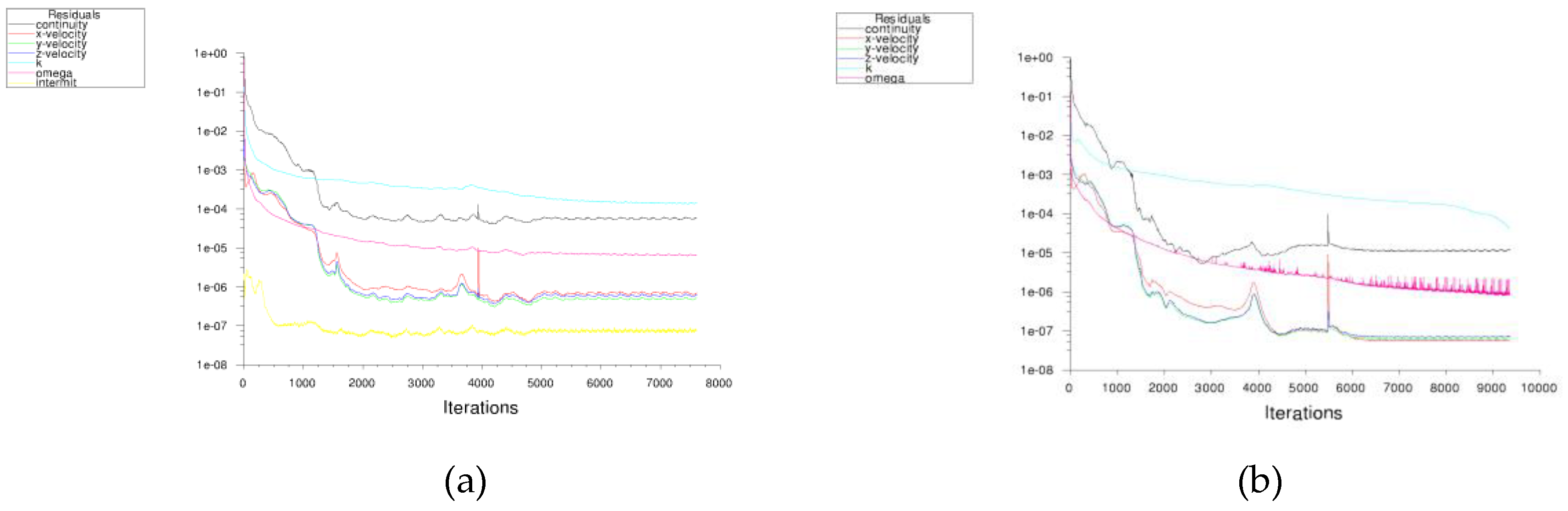
4.1. Convergence of the Solution

The flow solver has stable convergence behaviour. The steady computations were run generally for about 8000 iterations. An example convergence history of the residuals from the solved equations for a POT calculation with the γ-model and the SST model is given in Figure 3. As seen in the figure, the residuals for all the equations have dropped to a level below 10⁻⁴ as compared with their initial values. Therefore, the iterative solution is considered well converged after 8000 iterations.

4.2. In Open Water Conditions

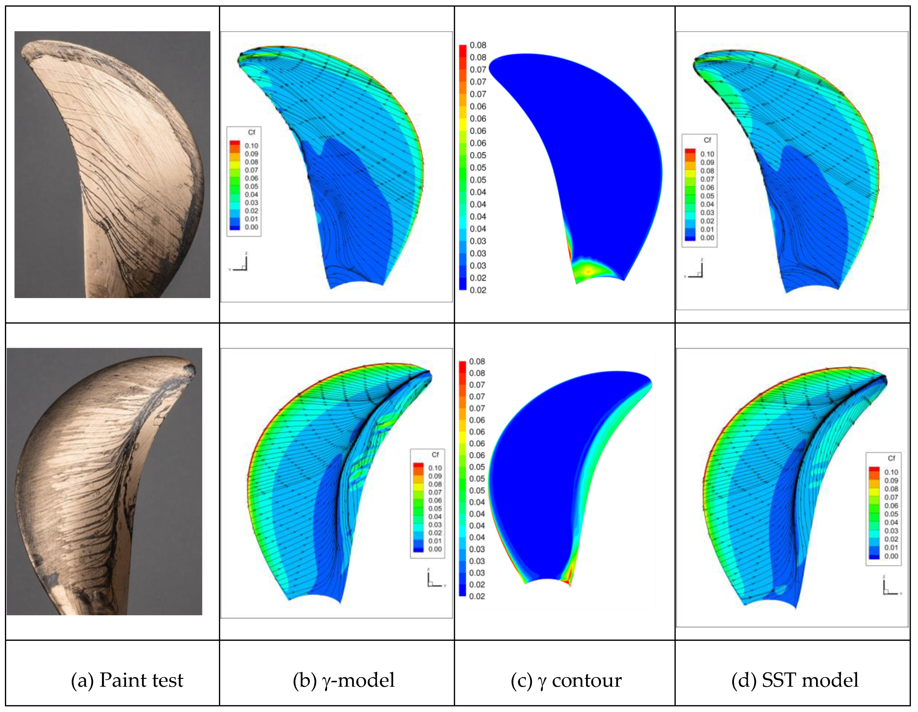
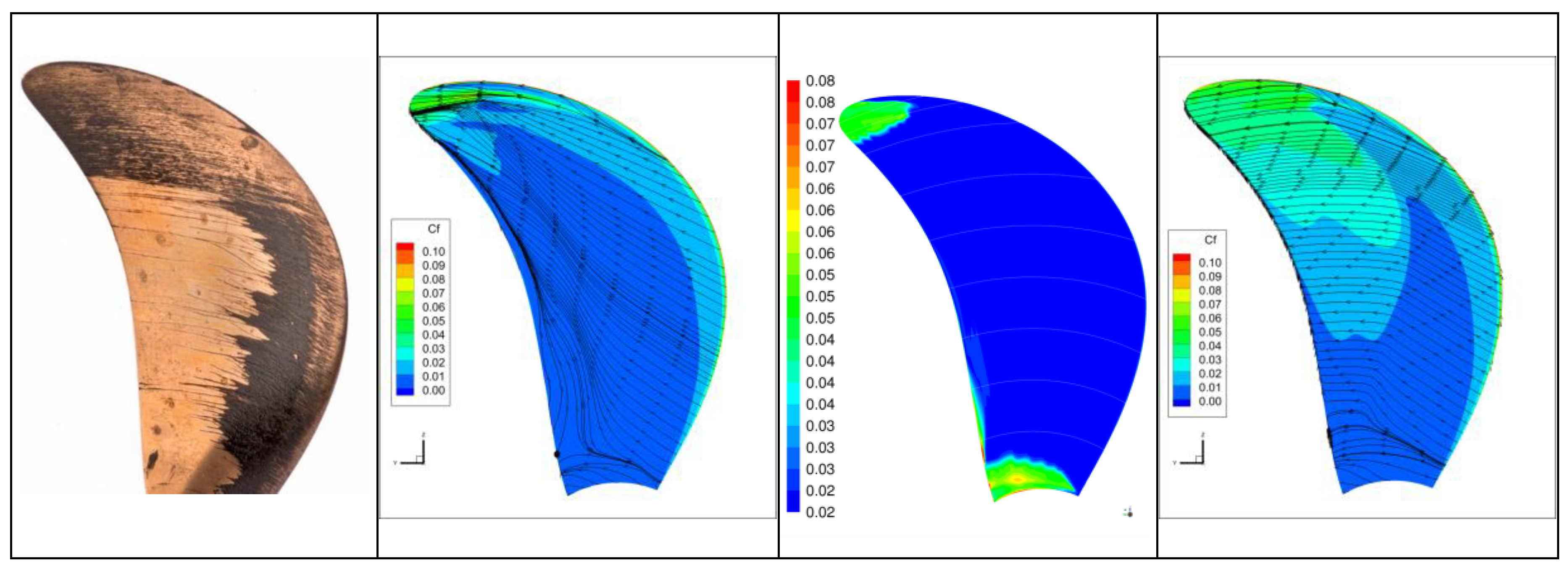
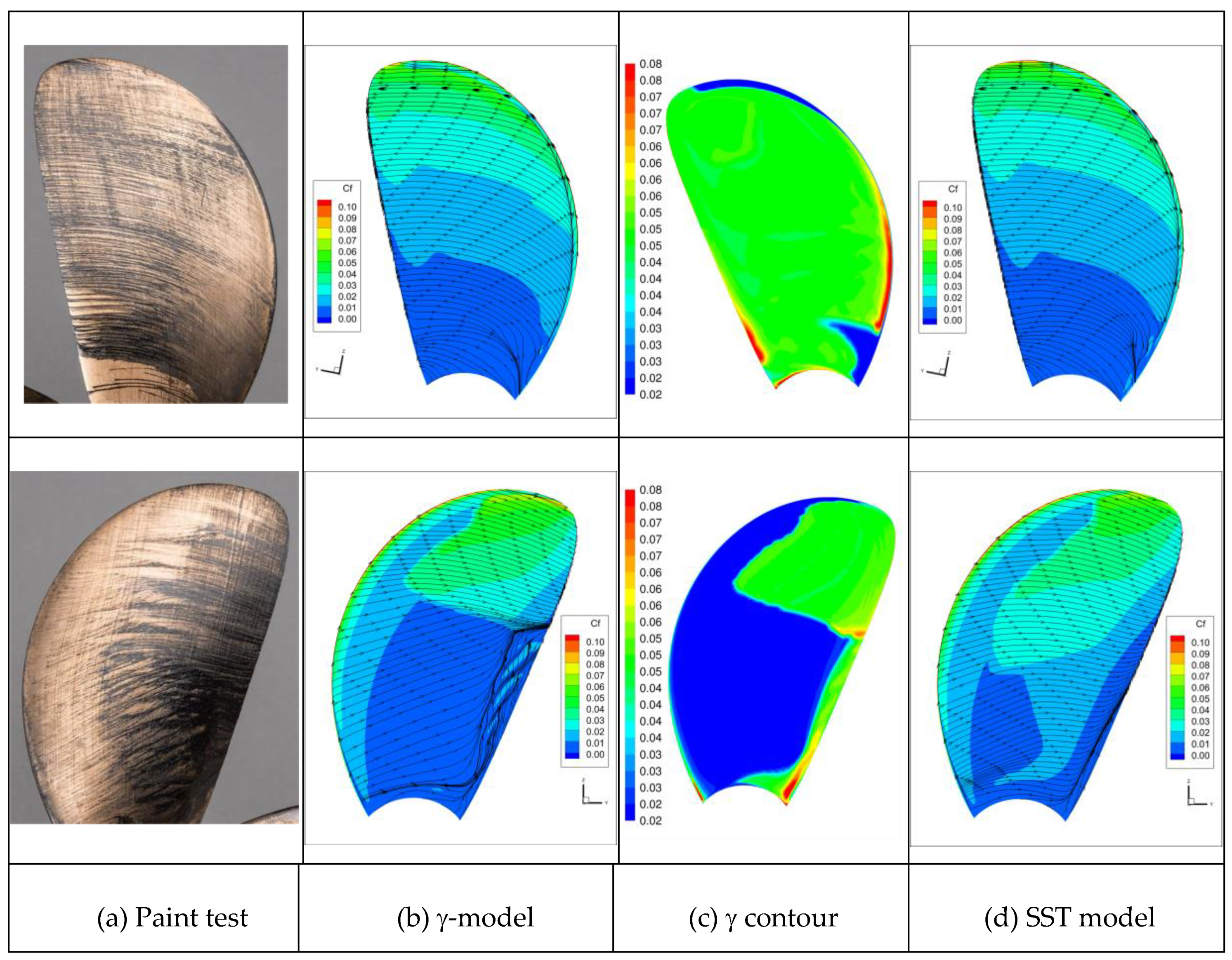
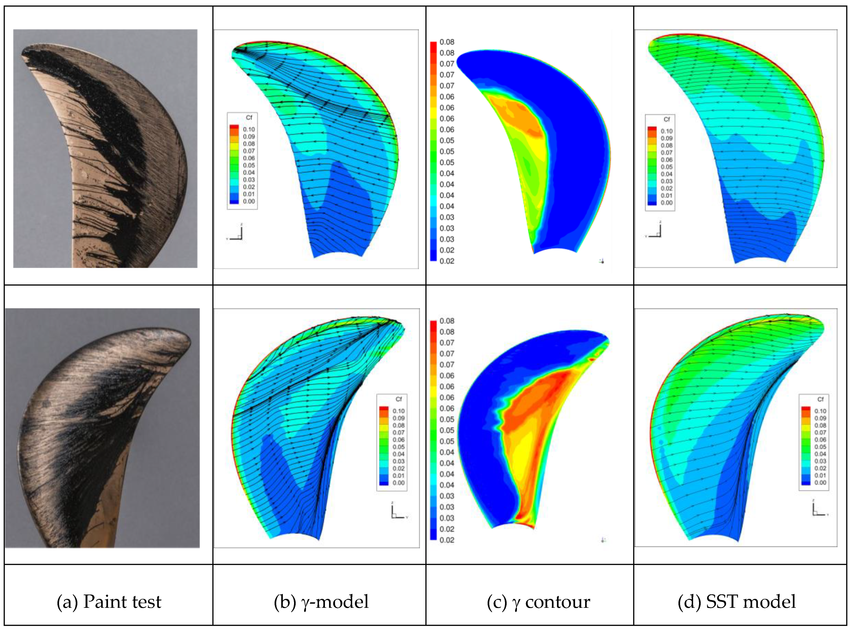
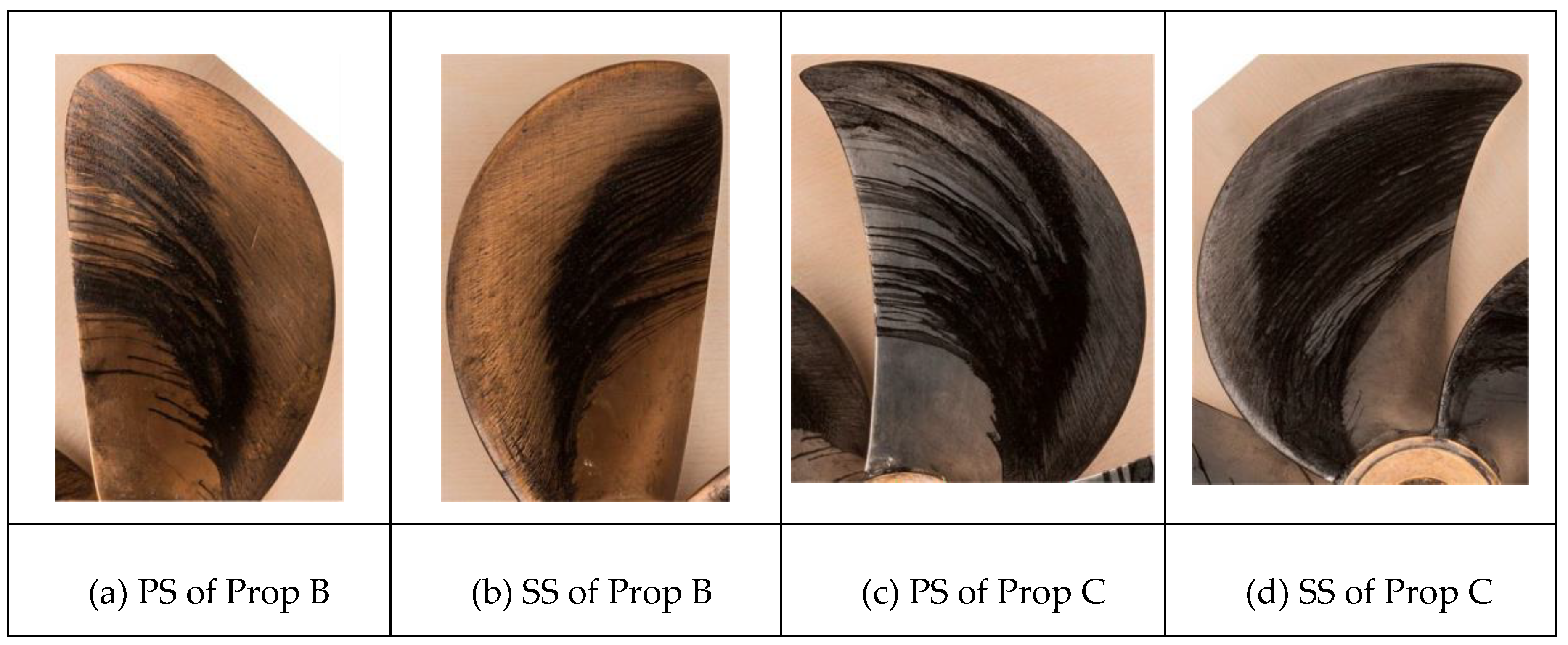
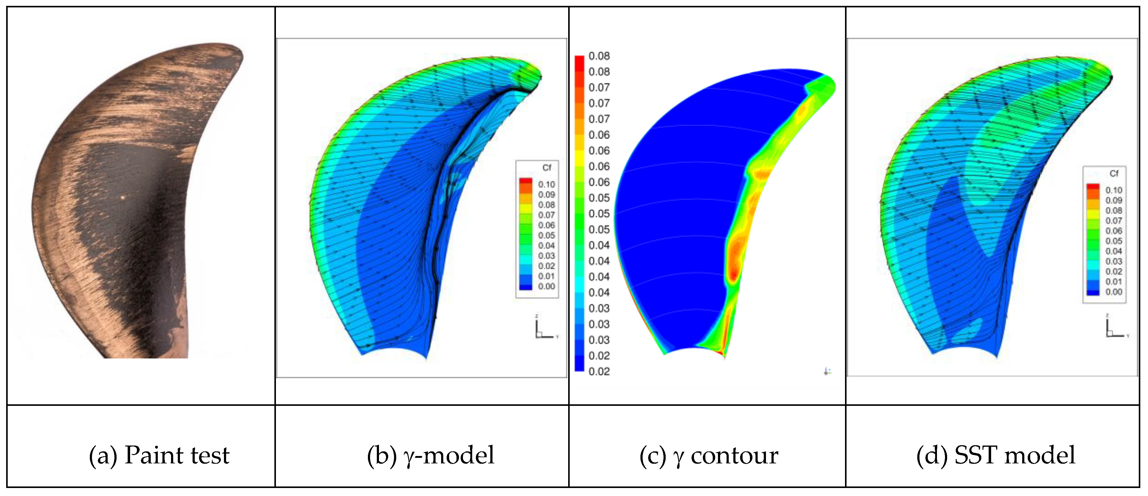
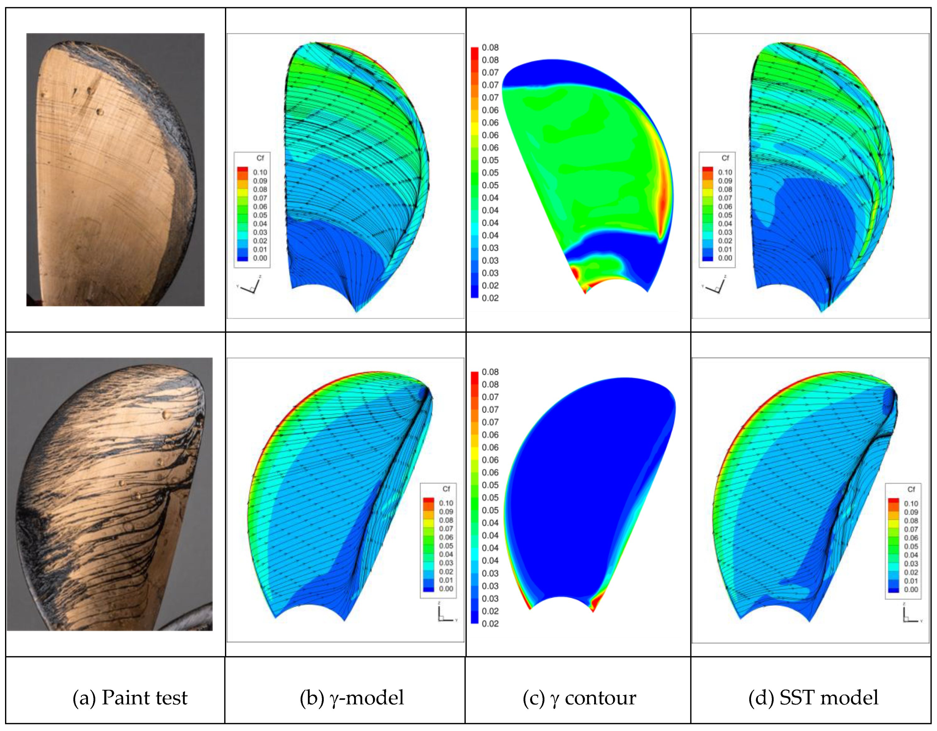
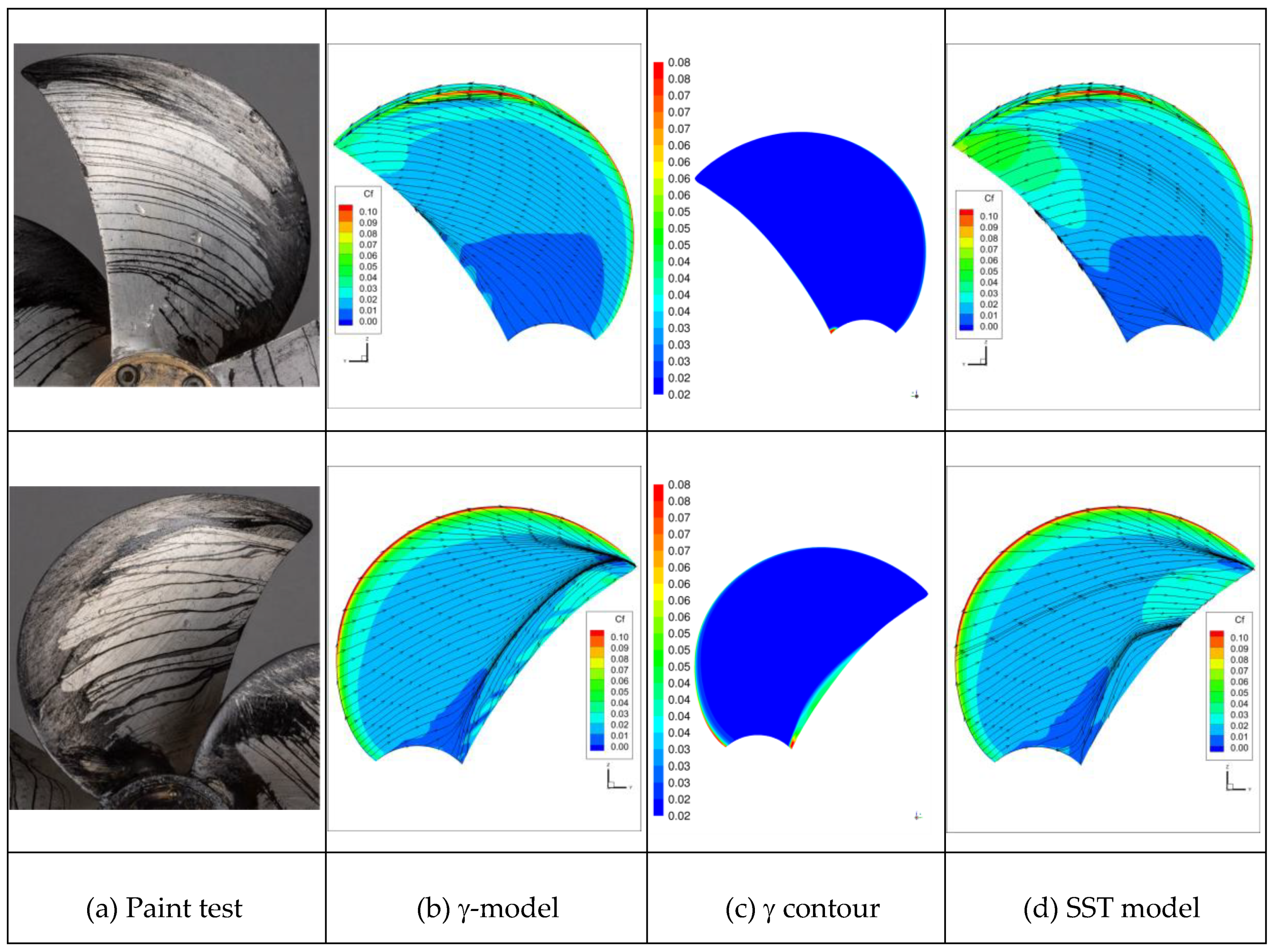
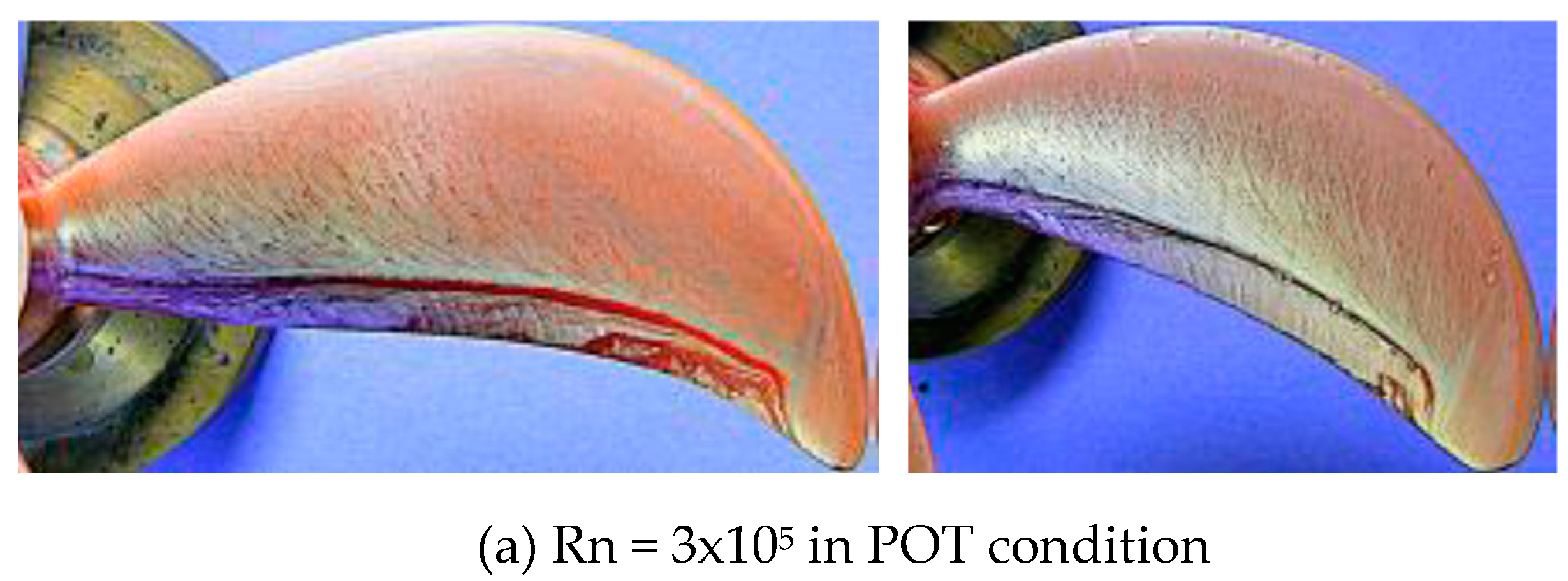
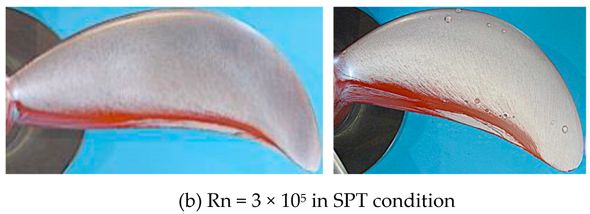
4.2.1. Paint Test vs. Predicted Near-Wall Flow

In each of the following figures (Figure 4, Figure 5, Figure 6, Figure 7, Figure 8 and Figure 9), paint test results are presented in the first column while a contour plot of the skin friction coefficient C_f overlaid by limiting streamlines is presented in the second column. The contour plot of turbulence intermittency γ in the range of 0.02 to 0.08 is displayed in the third column. The limiting streamlines by the SST model is shown in the fourth column. The turbulence intermittency of a value equal to or less than 0.02 is used for laminar regimes according to ANSYS Fluent, so any dark blue areas with γ ≤ 0.02 implies a laminar zone in the contour plot for γ. The value in the range γ = [0.02, 0.08] corresponds roughly to the transitional zone from laminar to turbulent flow. Values above 0.08 is regarded as turbulent flow.

Prop A

For Prop A, the RANS results are compared with the photos of the paint test in Figure 4 for the low Rn and Figure 5 for the high Rn condition. In the low Rn condition (Figure 4), the paint test reveals a strong radially-going flow on both sides of blades, which indicates a status of laminar flow. Near the trailing edge (TE) on the suction side (SS), the radially-going streamlines are concentrated at the ca 0.8C chordwise location, which shows the presence of a typical cross flow separation. A very similar pattern is reproduced by the γ-model. A transitional zone is visible on the SS near the TE and near the root on the pressure side (PS) for Prop A. The streamlines predicted by the SST model show a very good agreement with the paint test on SS but are somewhat different from the experiment on PS near the root and tip region. They exhibit a more tangentially going flow.

In the high Rn case (Figure 5), the paint test shows that the flow is directed more in the circumferential direction, especially at the outer radii SS, which indicates the expected turbulent flow structure. A large discrepancy is seen for the γ-model, which computed more radially-oriented streamlines on the PS. This means that the laminar flow region is overpredicted. On the SS close to the TE region, a strong radially-going flow and a flow separation along the TE are predicted by the γ-model, but no separation can be verified from the paint test result. In the outer blade area (0.75R< r < 1.0R), the paint test indicates a fully turbulent flow whereas the γ-model exhibits an overpredicted laminar flow on the SS. Compared with the γ-model, the SST model seems to have a closer agreement with the experiment for the high Rn condition.

Prop B

Limiting streamlines on Prop B are compared with the paint test results in Figure 6 for the low Rn case and compared with the paint results in Figure 7 for the high Rn condition.

In the low Rn POT case in Figure 6, the paint test reveals that the flow is going in the radial and tangential direction on both sides. Separation occurs on the SS at a distance upstream the TE and the separation line is parallel to the TE. This concentration of streamlines is well captured by the γ-model and SST model. The latter model gave a somewhat different pattern between the concentration line and TE. The streamlines show a slightly stronger radial orientation than the paint test traces. The models also predicted a reattachment along the LE on the PS. The intermittency quantity γ shows a transitional flow on a large part of PS and a laminar flow on SS.

In the high Rn condition (Figure 7), the streamlines on the inner blade area (with r < 0.65R) still have a radially orientated velocity component. The flow on the outer blade area, after a short transition distance from the LE, turns quickly to tangential (turbulent) flow. The intermittency contour plot shows a high amount of transitional/turbulent flow on the PS. There is about 40% transitional and 60% laminar flow on the SS. Compared with the SST model, the γ-model gives better agreement with the paint test on the SS.

Prop C

Limiting streamlines on Prop C are compared with the paint test results in Figure 8 for the low Rn case and in Figure 9 for the high Rn case. At low Rn, the paint traces imply the presence of both laminar and transitional flow on either side. On the SS, there are a few traces of flow separation before the flow reaches the TE. Compared with the paint test, the limiting streamlines by the γ-model demonstrate a stronger radial orientation, which means that the laminar part is over-predicted. This can also be seen from the intermittency contour plot (being entirely blue) in Figure 8c. The streamlines by the SST model exhibit some more transitional flow content near the TE on the outer blade. Both models predicted flow separation on the SS near the TE, but the separation line predicted by the SST model is shorter than that by the γ-model.

At the high Rn, more tangentially going streamlines are observed from the paint test, particularly on the PS. At the inner radii on the SS starting from the LE, some streamlines show a radial velocity component, which indicates a region of laminar flow. The limiting streamlines predicted by the γ-model are oriented more to the radial direction at the inner radii, which shows a dominance of laminar flow on the inner blade surface, whereas those predicted by the SST model appear to have closer agreement with the experiment. On the outer blade area, both models and the paint test suggest a fully developed turbulent boundary layer.

To summarize the prediction by the γ-model: at low Rn, the agreement with the paint test result is fairly good for Prop A and B, but is over-predicted in the laminar zone for Prop C. At high Rn, the agreement with the paint test is good for Prop B, but less satisfactory for Prop A and C where an overestimation of laminar flow is noted. Flow separation appears to be slightly over-predicted for all propellers at high Rn. The flow predicted by the SST model are similar with the γ-model for the low Rn cases. For the high Rn cases, the streamlines in the transition to the turbulence region correspond fairly well with the paint traces. The separation region predicted by the SST model is less than the prediction by the γ-model.

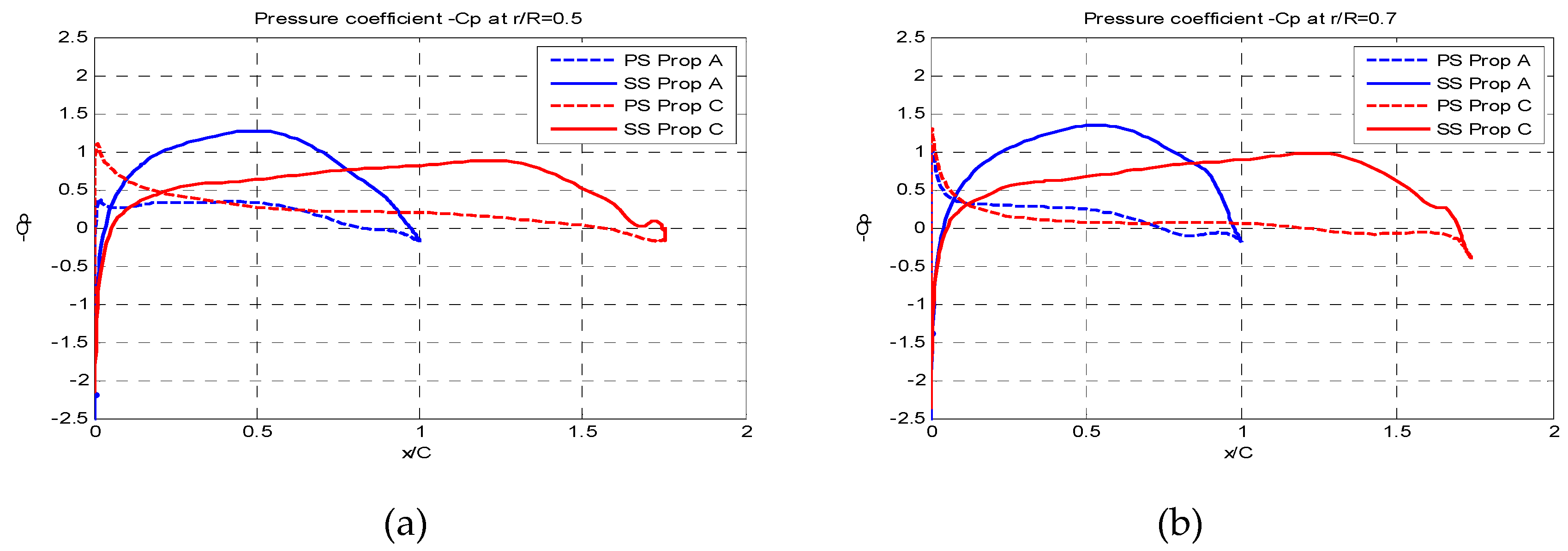
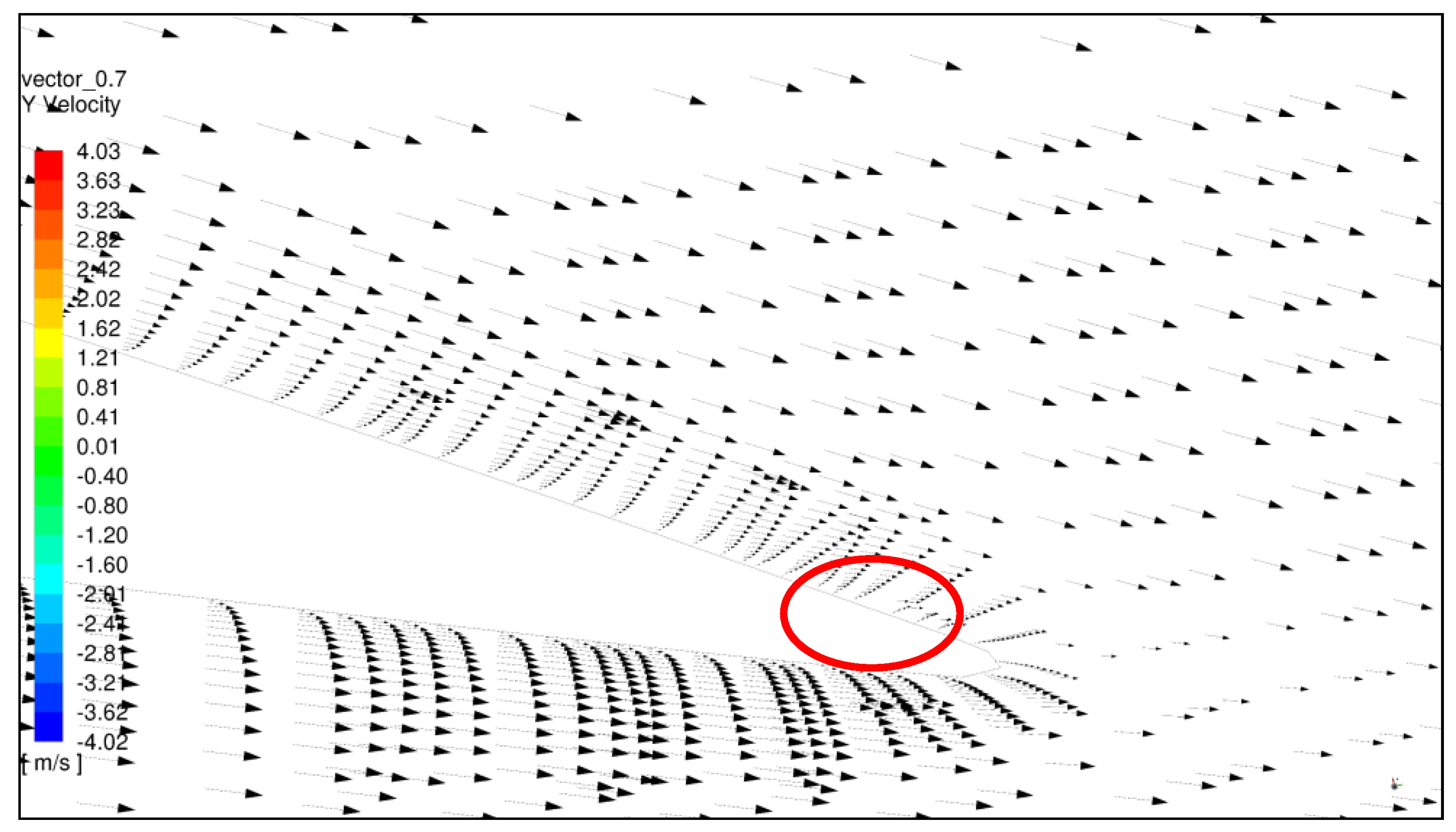
4.2.2. Flow Feature along Blade Sections

The pressure coefficients -C_p at blade section r = 0.5R and 0.7R, predicted by the γ-model in the low Rn case, are compared for Prop A and Prop C in Figure 10. The skin coefficients C_f at these sections are compared in Figure 11.

In Figure 10a, the non-dimensional chord length (x/C) of Prop C is rescaled along the abscissa with regard to that of Prop A, to show a relative length relationship with Prop A. The K_T for Prop C is a bit higher than Prop A, which means that the sectional loading on Prop C is higher than Prop A. However, looking at the downstream part of C_p curves for the two propellers in Figure 10a,b, we see that the adverse pressure gradient on the suction side (SS) of Prop A is relatively higher than Prop C. This is a rather significant difference between Prop A and C. It implies that Prop A is more prone to flow separation, particularly when the blade is working in a laminar flow that is highly sensitive to free-stream disturbance. Severe separation can be confirmed from the streamlines for Prop A in the paint test but not for Prop C (Figure 4 and Figure 8). From the C_f curves in Figure 11, we can see that the transition onset starts at a chordwise location at x/C≈ 0.70 for Prop A and x/C≈ 0.82 for Prop C.

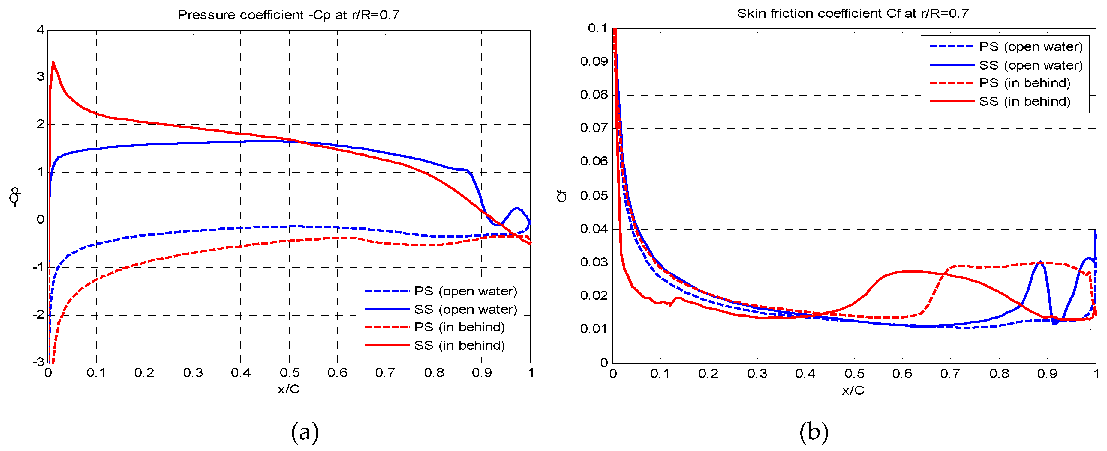
4.3. In Behind Condition

Paint tests of the propeller fitted to a ship model were conducted for all propellers but CFD computation was performed only for Prop A. It should be mentioned that the paint traces from the paint test in an SPT represent the averaged boundary layer flow characteristics resulting from many blade rotations and an inhomogeneous wake.

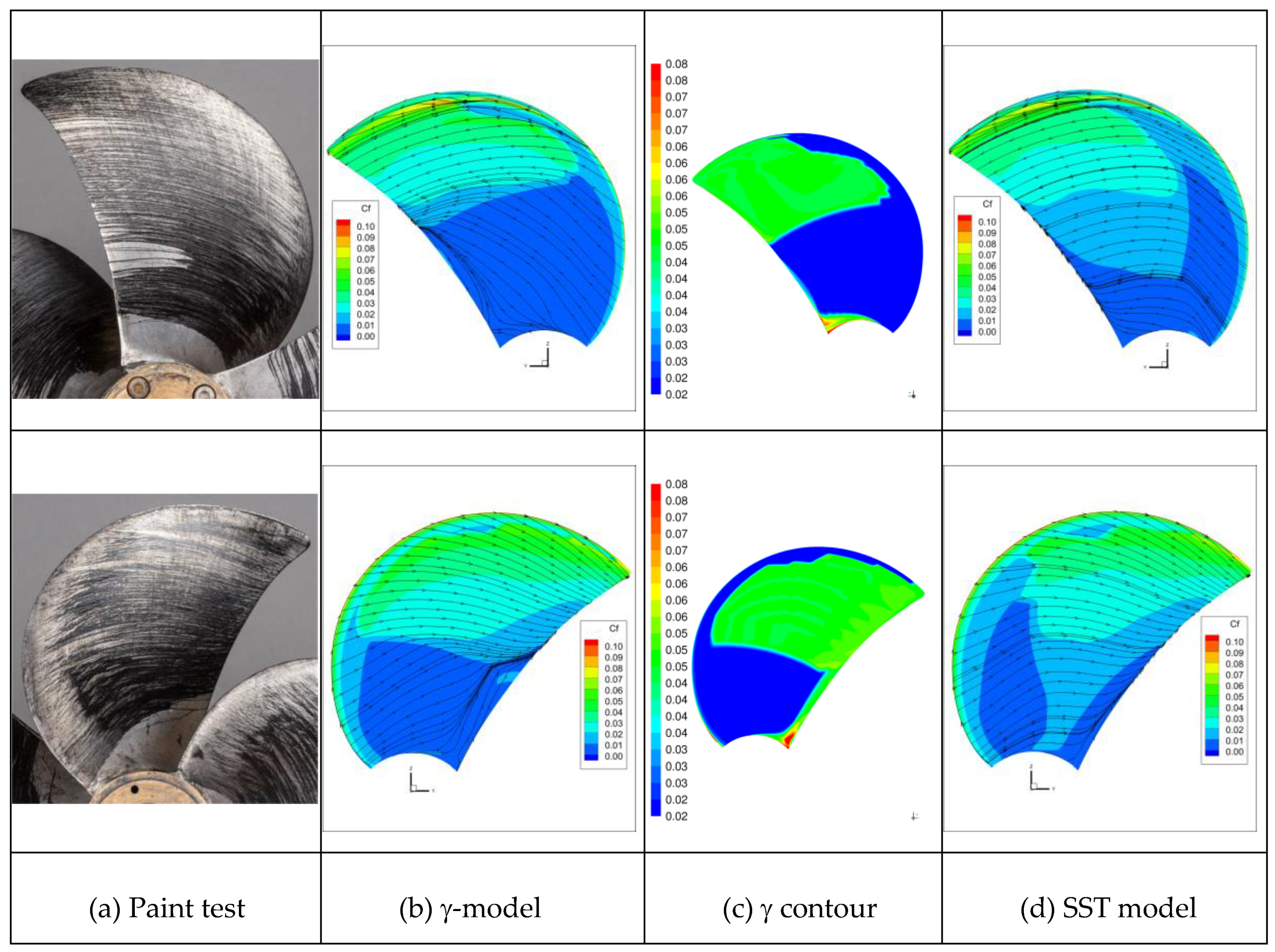
4.3.1. Paint Test Results and Predicted Streamlines

The paint test results for Prop A are compared with the limiting streamline predicted by the γ-model and the SST model in Figure 12. First, we noted from the paint test result that the near wall flow on the PS inner part of the blade goes more along the tangential direction than in the low Rn POT case (Figure 4a). Second, the near wall flow on the SS is similar yet different from that in Figure 4a. It has more radially-going content on the inner part of the blade, and more tangentially-orientated flow structure at the outer radii. The strong separation in parallel to the TE observed in the low Rn POT is not seen here. It is, however, not clear in the photo whether there is a separation near TE in the region 0.6R < r < 0.8R in Figure 12a. Similar characters were also reported by Hasuike et al. [5] and Lücke et al. [8]. The near wall flow pattern in the behind condition is much more complicated, due to a variable angle of attack to blade sections in the radial and circumferential directions, and a high turbulence level in the ship wake. The high turbulence intensity must have stabilized the flow to some extent but is not enough to change the boundary layer state from laminar to fully turbulent, so the blade is primarily covered with laminar and transitional flow.

The γ-model predicted a laminar flow in the outer blade area on the SS whereas the paint test revealed a turbulent flow in the region r > 0.9R. In the inner blade area, the trend is the opposite: the streamlines predicted by the γ-model exhibit a lesser extent of radial orientation compared with the paint test, which indicates an under-estimation of laminar flow and an earlier transition onset (Figure 12b). This feature can also be seen in the contour plot of intermittency in Figure 12c: the red area (high γ value) means a state of transitional/turbulent flow. The paint traces, however, indicated that the area is dominated by laminar flow. Nevertheless, compared with the SST model in Figure 12d, the γ-model has slightly closer agreement with the paint test.

Both the γ-model and the SST model predicted a flow separation near TE in the region with r < 0.75R, as implied by the converging streamlines in Figure 12b,d. In addition, the γ-model predicted an LE vortex separation and its subsequent reattachment along the LE at the outer radii with r > 0.75R.

The paint test results for Prop B and C are presented in Figure 13, and they are compared with the respective open water cases in Figure 6 and Figure 8. For Prop B, starting from LE, a laminar flow develops over about half of the blade area on the SS. Then the flow gradually changes direction toward circumferential, which indicates a transitional state of flow. However, unlike the open water case, no separation is observed in the behind condition. For Prop C, the paint traces have some similarity with those observed in the low Rn open water condition (Figure 8), yet have two discrepancies. They start with a clear and strong laminar flow pattern from the LE, spread about 1/4 chordwise over the blade. Then the flow direction is changed more rapidly to a circumferential region due to the disturbance of a high turbulence intensity in the wake. As a result, the flow over the rest of 3/4 blade area exhibits a transitional flow character. No separation is found on the SS.

To summarize the paint test results for propellers in low-Rn open water and in the behind conditions, we noted that the near wall flow is still dominated by laminar and transitional content in the behind condition, but the amount of laminar flow has decreased and the amount of turbulent flow increased. For the two high blade area propellers (B and C), there is no separation on SS. Although separation cannot be verified for Prop A from the present paint test result, both the oil flow visualization and computational results from Hasuike et al. [3,4,5] confirmed that flow separation is constantly present in SPT for low blade area propellers. Examples of oil flow visualization from [5] are given in Figure 14 for two narrow blade propellers tested in POT and SPT conditions. The paint tests carried out at HSVA [8] also revealed such a difference between low and high blade area propellers. We believe that flow separation in SPT has made a low blade area propeller different from a high blade area propeller. The large blade-thickness-to-chord ratio and the high adverse pressure gradient near the TE of the low blade area propellers have made the blade more vulnerable to laminar flow separation. It is likely that the flow separation has resulted in an increased pressure drag, which leads to a higher K_Qb in the behind condition. This may have played a role for the unexpected drop of η_R when the standard ITTC-78 method is used. (to be explained further in §4.5)

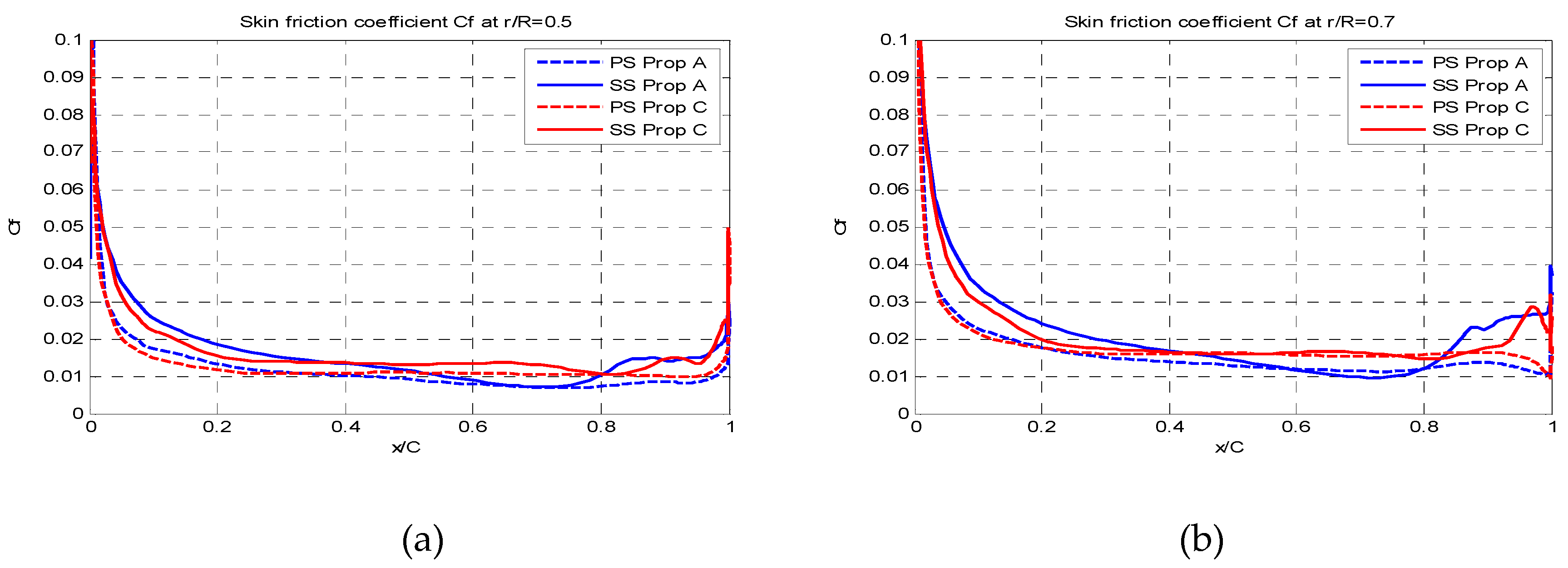
4.3.2. Flow Feature along Blade Sections

The pressure (C_p) and skin friction coefficient (C_f) at blade section r = 0.7R of Prop A is shown in Figure 15, and they are compared with the values in the open water case at the same J-value. Due to a higher angle of attack to blade sections when the propeller works behind the ship wake, the C_p envelop in the open water and the behind condition (Figure 15a) looks somewhat different but the integration over the entire blade should lead to the same K_T for the two cases. Compared with the C_f in an open water case (blue lines) in Figure 15b, the transition location is moved upstream to x/C≈0.42 on the SS and x/C≈0.64 on the PS in the behind condition (red lines), due to the increased turbulence intensity level in the ship wake as well as a difference in the angle of attack. It means that the near wall flow feature in POT and SPT is different despite the fact that the propeller is operating at the same Rn.

The velocity vector at a cylindrical surface of radius r = 0.7R is plotted in Figure 16, which shows the flow field near the TE of that blade section. On the SS near wall region, the velocity vectors look shorter than those on the PS because the flow has a radially-going component (i.e., the cross-flow component) not visible on the plotting plane. Separation took place near the TE on the SS, as marked by the red oval in the figure. The vector plot reveals the same character as shown in Figure 12b from another perspective.

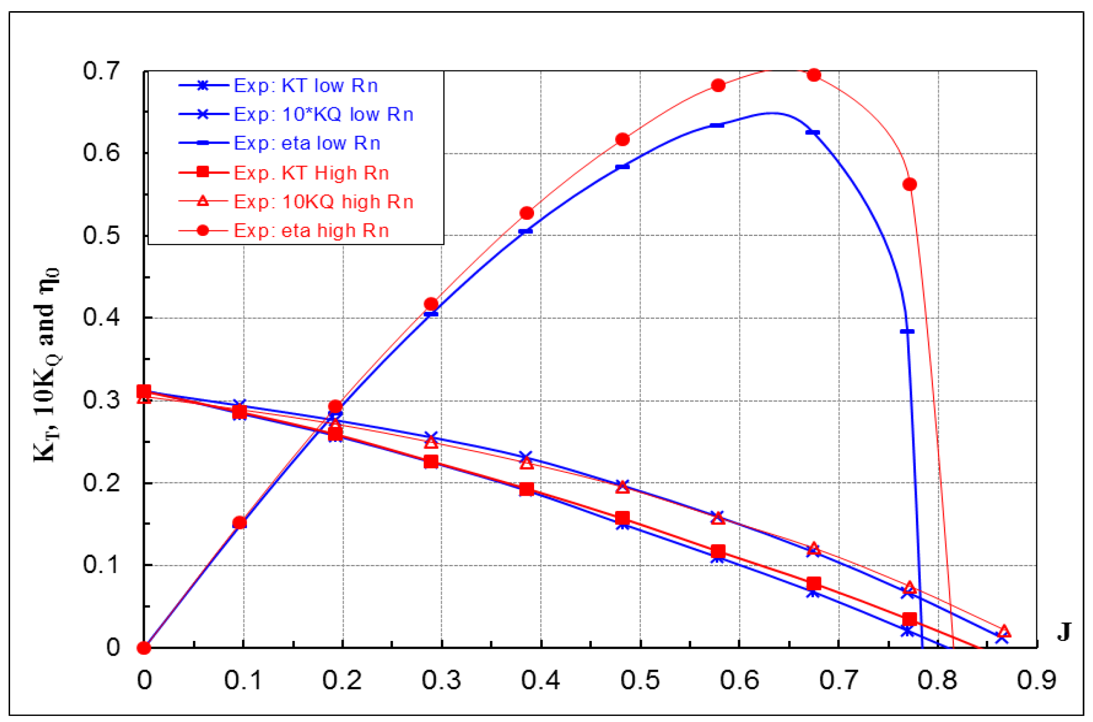
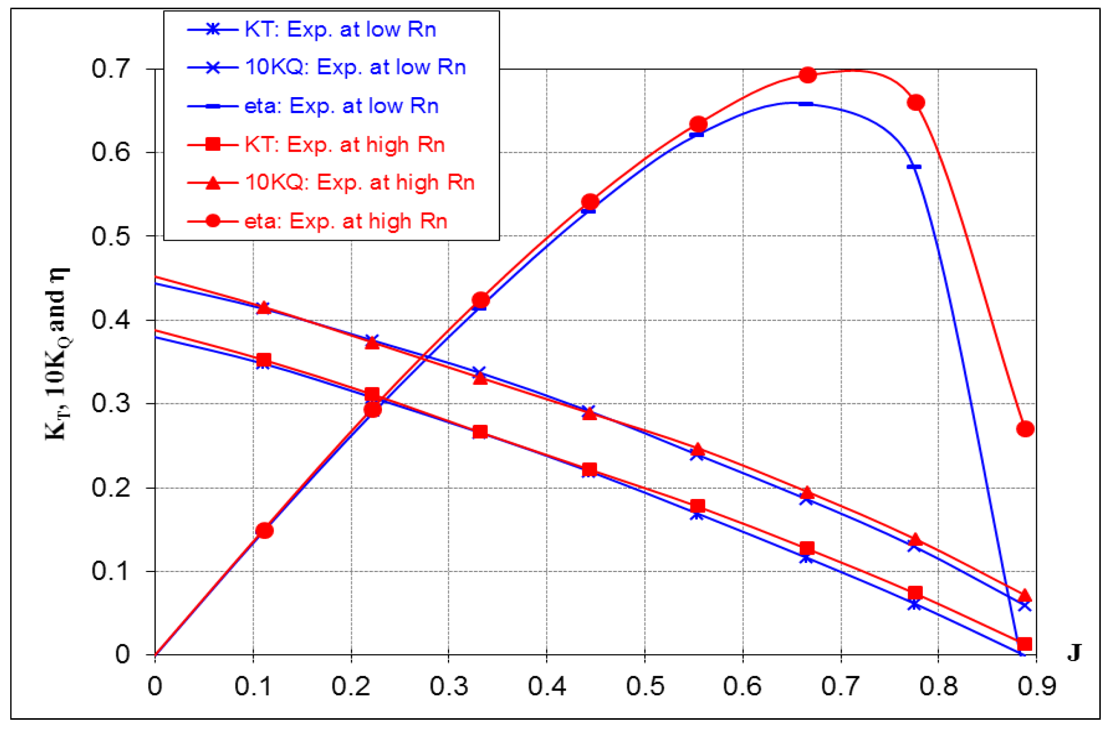
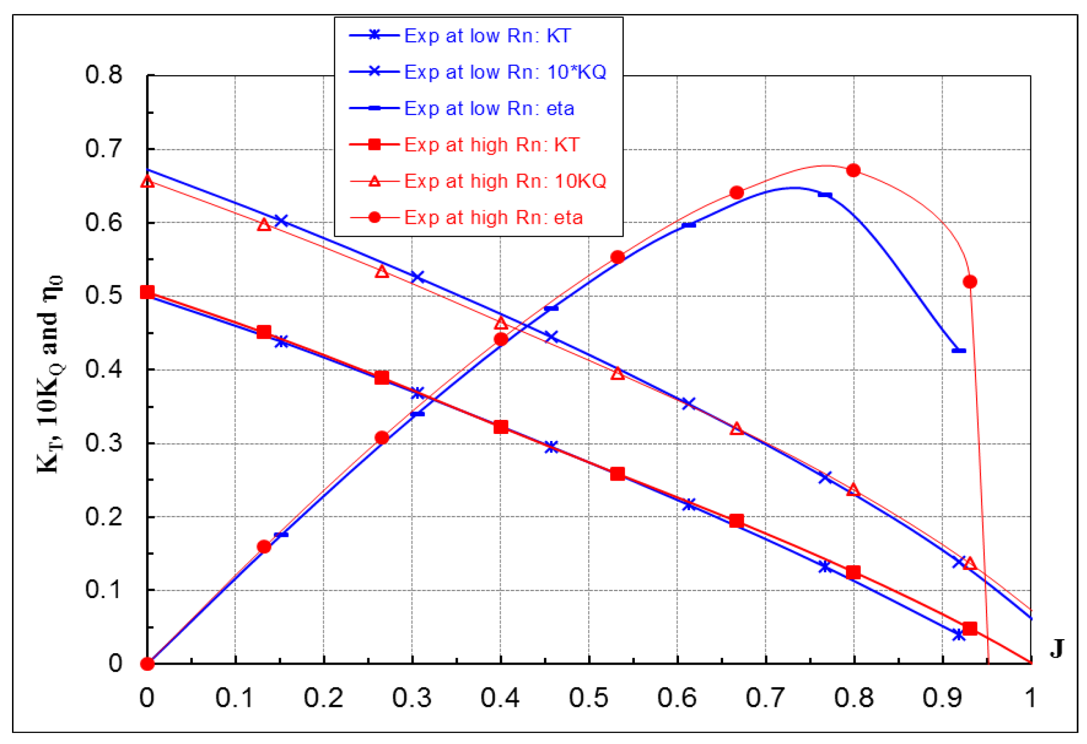
4.4. POW Characteristics at Two Rn Numbers

To show the difference in POW between two POTs tested at a low Rn and a high Rn (see Table 2 for the Rn difference), the measured POW data for Prop A, B, and C are presented in Figure 17, Figure 18, and Figure 19, respectively.

For Prop A, the K_Q at the low Rn is slightly higher than in the high Rn case for the lower half of the advance-ratio (J) range, ca J < 0.50. The K_Q becomes lower in the high J-range. Difference in K_T occurs only in the high J-range, where K_T at the low Rn is lower. For Prop B, the scale effect occurs mainly in the J-range of J > 0.45 where both K_T and K_Q at the low Rn are a bit lower than those at the high Rn, which is a typical sign that the propeller tested in the low Rn case is working below the critical Reynolds number. For Prop C, K_Q at the low Rn is higher than that at the high Rn in the range of J < 0.6. K_T and K_Q at the low Rn are lower than those at the high Rn for the range with J > 0.6. The response of POW to the Rn variation is clearly dependent on the propeller design. Different propellers exhibit different extent of scale effects due to a moderate change of Rn. Assuming a propeller is normally operated in an open water efficiency range of 0.45 < η₀ < 0.65 in model tests, the difference in K_T (and K_Q) between the two sets of POW is not greater than 2.5%. The difference in η₀ can be larger, e.g., for Prop A, and η₀ is always higher at the high Rn.

The K_T and K_Q predicted by the RANS method for the same J values as in the paint tests are presented for the γ-model in

Table 4. POW predicted by the γ-model.

Prop	Rn [x105]	J	KT [-]	10KQ [-]	ηo [-]	ΔKT [%]	ΔKQ [%]	Δηo [%]
A	2.06	0.646	0.077	0.122	0.650	−4.3	−6.3	2.2
	5.08	0.646	0.088	0.126	0.715	−2.7	−4.8	2.2
B	2.15	0.694	0.098	0.169	0.642	−4.5	−2.4	−2.2
	6.46	0.694	0.109	0.179	0.671	−3.6	−1.4	−2.2
C	2.24	0.824	0.099	0.203	0.638	1.4	−3.5	5.1
	6.71	0.824	0.101	0.212	0.627	−9.2	−3.5	5.9

and for the SST model in

Table 5. POW predicted by the SST k-ω model.

Prop	Rn [x105]	J	KT [-]	10KQ [-]	ηo [-]	ΔKT [%]	ΔKQ [%]	Δηo [%]
A	2.06	0.646	0.072	0.115	0.641	−10.4	−11.3	1.0
	5.08	0.646	0.081	0.122	0.682	−9.8	−7.5	−2.5
B	2.15	0.694	0.103	0.174	0.654	0.4	0.8	−0.4
	6.46	0.694	0.106	0.176	0.665	−5.9	−2.9	−3.1
C	2.24	0.824	0.097	0.203	0.629	−0.3	−3.6	3.5
	6.71	0.824	0.098	0.206	0.626	−12.0	−6.3	−6.0

. The errors (ΔKT, ΔKQ, and Δη_o) relative to experimental data, defined as e.g., ΔKT = (K_{T_cfd}/K_{T_exp} -1), are also shown in the tables. It is seen that both models underpredict the K_T and K_Q, but the POW predicted by the γ-model has slightly closer agreement with the measured data than the SST model. On the other hand, considering that the J values in these computations are off-design values located in the high-J range. A large deviation of computed POW is, to some extent, expected. For Prop A and Prop B, the prediction errors of the γ-model are larger in the low Rn case than the high Rn case. Detailed analysis of computational results is beyond the scope of the paper and will be discussed in another paper.

4.5. Influence on Performance Prediction

An unusual low value of η_R is sometimes obtained when the ITTC-78 method is used in the performance prediction for low blade area propellers, as reported by Tsuda et al. [2] and Hasuike et al. [3,4,5]. The authors attributed this phenomenon to a Reynolds number (Rn) difference between the POT and the SPT. This is certainly one reason. However, there might be other reasons.

In

Table 6. ITTC-78 vs. 2POT predicted propulsive factors.

Prop	Case	Method	Vs [kn]	POT at	nm [1/s]	ηom [-]	ηR [-]	ηH [-]	Ship ηo [-]	Ship ηD [-]
A	1a	ITTC-78	14.5	high Rn	8.1	0.540	0.991	1.170	0.614	0.711
	1b	2POT	14.5	low Rn	8.1	0.508	1.029	1.180	0.610	0.741
B	2	ITTC-78	14	high Rn	6.6	0.575	1.022	1.224	0.631	0.790
	3	ITTC-78	14.5	high Rn	7.4	0.592	1.019	1.149	0.634	0.742
	4	ITTC-78	15	high Rn	7.5	0.609	1.023	1.145	0.647	0.758
C	5	ITTC-78	24	high Rn	8.9	0.657	1.020	1.080	0.689	0.759
	6	ITTC-78	22	high Rn	9.6	0.614	1.021	1.119	0.648	0.740

, the propulsive efficiency factors predicted by the ITTC-78 method and the 2POT method (for Prop A in one project) are presented for a few cases where these propellers are used in the SPT in a number of projects. The Rn level used in the POT is marked with low Rn or high Rn. The n_m in the table is the rate of revolution during SPT. Note that, except for Prop A, each case for Prop B and Prop C was extracted from a different project with a different ship model. It represents the result at the design speed of the vessel in that project. There is no connection between cases, except for Case 1a and Case 1b of Prop A, which are from the same project and the same vessel.

For Prop A, we see in Table 6 (Case 1a) an unusual low η_R (η_R = 0.991) is obtained when the ITTC-78 method is used. Using the 2POT method with a POT tested at a low Rn, an expected level of magnitude is obtained, i.e., η_R =1.029 (Case 1b). This is the situation with the low blade area propeller. If we now look at the two conventional propellers, B and C, they are both run at about the same low Rn as Prop A during SPTs for all the cases (Case 2–6). POT is run at a high Rn and the standard ITTC-78 method is applied. In all these cases, the predicted η_R has an expected order of magnitude. From the POW curves in Figure 18 and Figure 19, we see that there is also some Rn scale effect on Prop B and C, particularly for Prop C, but why is it that Prop B and Prop C do not suffer from the drop of η_R? The answer is related to the flow separation phenomenon in SPT for the low blade area propellers, as discussed in Section 4.3.2. We observed a significant difference between the low and the high blade area propeller from the paint test result in SPT. Flow separation is present on the SS of the low blade area propeller but no separation on the high blade area propellers is present. For airfoils, laminar flow separation on the suction side leads to reduced lift and increased pressure drag. The same applies for propeller blades. The separation reduces the thrust and increases the torque. To generate the required thrust, a propeller suffering flow separation must rotate at a bit higher rpm, which results in a slightly lower J value and a lower efficiency of the propeller. The low open water efficiency value of η_om in Table 6 for Prop A indicates that the Prop A seems to work less efficiently in model scale, when compared with Prop B and Prop C.

There are two factors that can lead to a decrease of η_R: (a) A difference in POW curve due to an Rn difference in a POT and an SPT, and (b) flow separation on blades during an SPT. As per definition, the relative rotative efficiency η_R is defined as:

$${\mathsf{\eta }}_{\mathrm{R}}=\frac{{\mathrm{K}}_{\mathrm{Q}0}}{{\mathrm{K}}_{\mathrm{Q}\mathrm{b}}}$$

(1)

where K_Q0 is the torque coefficient interpolated from the POW curve using the K_T-identity method and K_Qb is the measured torque coefficient during the SPT. If a POW curve from a POT carried out at a high-Rn is used for interpolation in the ITTC-78 method, the minor Rn difference between POT and SPT can give rise to a lower K_Q0, which leads to a decrease of η_R. On the other hand, a higher K_Qb can also lead to a drop of η_R. Occurrence of flow separation near the TE implies a higher pressure drag on blades and, hence, an increased K_Qb, which leads to a lower η_R. In reality, both a higher K_Qb in SPT and a lower K_Q0 interpolated from a POT tested at a high Rn might have collaboratively resulted in a decrease of η_R. The two conventional propellers do not suffer from this issue despite working at the same Rn as Prop A in SPT because their near-wall flow is not separated in the SPT due to a longer chord length and a gradual change of the adverse pressure gradient on the SS. Both factors are closely related to Rn scale effects, but what makes the difference in response to a moderate Rn variation in POT and SPT among different propellers is the design philosophy. If separation is the decisive factor on the change of η_R, in principle, any propeller that suffers from laminar separation in an SPT will likely get a low η_R with the ITTC-78 method. Therefore, this phenomenon does not necessarily occur only on low blade area propellers, and it can happen to other propellers. So far, it seems that low blade area propellers suffer more from the Rn scale effects than conventional propellers.

Using a POW curve from a low-Rn POT will influence the intersected J_Tm and K_Q0. It generally leads to a slightly higher η_R and a higher hull efficiency η_H, a slightly lower J_Tm and η_mo, and a few percentage increase of η_D. The consequence of applying the 2POT method can be seen in Table 6. The 2POT method may be able to bring the η_R back to a normal value for the low blade area propellers. However, the previous work by others [2,8] and SSPA’s paint test results find that the near wall flows in the POT and SPT, performed at the same Rn, show a similarity of laminar flow character, but also reveal some differences in the flow orientation. The high turbulence intensity in ship wake has made the flow more transitional and turbulent. The shift of the transition onset location towards LE in the SPT discussed in Section 4.3.2 is clear evidence of such a difference. This means that, if a 2POT method is to be adopted, a somewhat higher Rn than that used in SPT should be chosen for use in the low Rn POT test, in order to achieve some consistency for the near-wall flow between the POT and SPT. This calls for a thorough calibration work like the one mentioned in Reference [8].

On the other hand, we have to be aware the disadvantages in model testing with the 2POT method. For example, it can be troublesome to carry out a model test in laminar and transitional flow regimes, as this type of flow is very sensitive to a change of model speed (hence, Rn number), which sets a very high requirement on the accuracy of the model speed. Laminar flow is vulnerable to the free-stream turbulence disturbance and is prone to separation. Testing in a laminar/transitional flow regime may result in flow instability and oscillating forces, and it requires special equipment to measure the forces reliably. Therefore, it is preferable not to perform a model test in the low-Rn laminar flow regime (unavoidable for SPT). This was one of the reasons to require that a POT be performed at an Rn higher than the critical Rn_c when the ITTC-78 method was developed. The challenge that ITTC members are facing is whether a better scaling method or a modified ITTC-78 method can be developed for non-conventional propellers in the future. Some initial work has just been started at SSPA.

5. Conclusions

The aim of this work was to explain the causes of the unexpected low value of η_R resulted from the scaling of model test result with the ITTC-78 method for the low blade area propellers. Model testing and a RANS method with the intermittency transition γ-model were used to study the near-wall flow characteristics in open water and behind conditions for three propellers, which represent a modern low blade area design (Prop A) and two conventional designs (Prop B and Prop C).

For the open water tests at the low Rn, the paint test results show a laminar flow dominance on blades for all the propellers. Separation is observed on the SS of Prop A and Prop B. For the POT at the high Rn, the near wall flow is a combination of laminar, transitional, and turbulent flow. There is no separation on the SS for all the propellers during the POT at the high Rn.

In the behind condition, the paint tests show that laminar and transitional flow coexist, and the amount of laminar flow has decreased. No separation occurs on Prop B and Prop C. It is unclear from the paint test if there is a separation on the SS of Prop A, but the CFD result predicts a flow separation for this propeller. SSPA’s paint test results showed a similar tendency as observed at HSVA regarding the different response to the Rn difference in POT and SPT tests for the low and high blade area propellers.

We observe that two factors can lead to a decrease of η_R for low blade area propellers. (a) A moderate difference in Rn between the POT (following standard ITTC-78) and SPT that causes a small difference in POW curves. (b) The flow separation on the SS of the blade near TE. Both phenomena are caused by the Reynolds scale effects. If the experiment had been done at full scale, the phenomena would not have happened. Furthermore, the occurrence of the unexpected low η_R is closely associated with design philosophy like the blade section profile, length, thickness-to-chord-ratio, and chordwise load distribution.

The 2POT method offers a solution to bring back a too-low η_R for low blade area propellers, as it attempts to make the boundary layer state (Rn) in a POT similar with that in an SPT. If an unusual drop of η_R is observed in a prediction with the ITTC-78 method, the 2POT method may be considered as an alternative method to predict propulsive efficiency factors for propellers that suffer from the η_R problem. However, if the 2POT method is used for power performance prediction, then the correlation factors like C_N and C_P need to be re-established. With the awareness of the potential problems with the 2POT method (discussed in Section 4.5), we encourage the continuing effort in the ITTC committees and member society to develop new scaling methods for unconventional propellers. Some initial work has been started at SSPA.

The limiting streamlines predicted by the γ-model do not always agree well with the paint test results in the computed cases. An overpredicted laminar zone and delayed transition onset are observed for Prop A in the high Rn case, for Prop B in the low Rn case, and for Prop C at both Rn numbers. The inconsistency in streamline prediction is partially associated with the sensitivity of the transition model to the free-stream turbulence quantities at the inlet, and partly caused by numerical errors. The latter issue will be discussed in a separate paper. Overall, the streamlines predicted by the γ-model have slightly better agreement with the paint tests compared with the SST model in the low Rn cases. Using the turbulence intermittency threshold value as an indicator, the amount of laminar flow area on blade surfaces can be quantified approximately with the γ-model. This information confirms the laminar flow dominance on blades for all propellers at low Rn. Transition models are known to be sensitive to Tu and TVR prescribed at the velocity inlet boundary. Without the correct info of Tu and TVR at some distance upstream of the propeller LE, it is difficult for a transition model in its present form to accurately predict the onset of transition and skin friction at a low Rn. Nevertheless, a transition model provides a qualitatively better insight in the near-wall flow on blades than a fully turbulence model.

The paint test is still the most reliable and efficient method to detect the presence of laminar and turbulent flow, the onset of transition, and the occurrence of flow separation. One future work is to study the near wall flow with the present method for a propeller with other section profiles such as an Eppler-like section.

References

1. Tamura, K.; Sasajima, T. Some Investigations on Propeller Open-Water Characteristics for Analysis of Self-Propulsion Factors; Mitsubishi Heavy Industries, Ltd.: Tokyo, Japan, 1977. [Google Scholar]
2. Tsuda, T.; Konishi, S.; Asano, S.; Ogawa, K.; Hayasaki, K. Effect of propeller Reynolds number on self-propulsion performance. Jpn. Soc. Nav. Archit. Ocean Eng. 1978, 169, 127–136. [Google Scholar]
3. Hasuike, N.; Okazaki, A.; Yamasaki, S.; Ando, J. Reynolds effect on Propulsive Performance of Marine Propeller Operating in wake flow. In Proceedings of the 16th NuTTS 2013, Mulheim, Germany, 2–4 September 2013. [Google Scholar]
4. Hasuike, N.; Okazaki, M.; Okazaki, A. Flow characteristics around marine propellers in self-propulsion test condition. In Proceedings of the 19th NuTTS, St. Pierre d’Oleron, France, 3–4 October 2016. [Google Scholar]
5. Hasuike, N.; Okazaki, M.; Okazaki, A.; Fujiyama, K. Scale effects of marine propellers in POT and self-propulsion test conditions. In Proceedings of the 5th International Symposium on Marine Propulsors, SMP’17, Espoo, Finland, 12–15 June 2017. [Google Scholar]
6. Streckwall, H.; Lucke, T.; Bugalski, T.; Felicjancik, J.; Goedicke, T.; Greitsch, L.; Talay, A.; Alvar, M. Numerical Studies on Propellers in Open Water and behind Hulls aiming to support the Evaluation of Propulsion Tests. In Proceedings of the 19th NuTTS, St. Pierre d’Oleron, France, 3–4 October 2016. [Google Scholar]
7. Helma, S. An Extrapolation Method Suitable for Scaling of Propellers of any Design. In Proceedings of the 4th International Symposium on Marine Propulsors, SMP’15, Austin, TX, USA, 1–4 June 2015. [Google Scholar]
8. Lücke, T.; Streckwall, H. Experience with Small Blade Area Propeller Performance. In Proceedings of the 5th International Symposium on Marine Propulsors, SMP’17, Espoo, Finland, 12–15 June 2017. [Google Scholar]
9. Heinke, H.J.; Hellwig-Rieck, K.; Lübke, L. Influence of the Reynolds Number on the Open Water Characteristics of Propellers with Short Chord Lengths. In Proceedings of the 6th International Symposium on Marine Propulsors, SMP’19, Rome, Italy, 17–21 May 2019. [Google Scholar]
10. Bhattacharyya, A.; Neitzel, J.C.; Steen, S.; Abdel-Maksoud, M.; Krasilnikov, V. Influence of Flow Transition on Open and Ducted Propeller Characteristics. In Proceedings of the 4th International Symposium on Marine Propulsors, SMP’15, Austin, TX, USA, 1–4 June 2015. [Google Scholar]
11. Bhattacharyya, A.; Krasilnikov, V.; Steen, S. A CFD-based scaling approach for ducted propellers. Ocean Eng. 2016, 123, 116–130. [Google Scholar] [CrossRef]
12. Bhattacharyya, A.; Krasilnikov, V.; Steen, S. Scale effects on open water characteristics of a controllable pitch propeller working within different duct designs. Ocean Eng. 2016, 112, 226–242. [Google Scholar] [CrossRef]
13. Sánchez-Caja, A.; González-Adalid, J.; Pérez-Sobrino, M.; Sipilä, T. Scale Effects on Tip Loaded Propeller Performance Using a RANSE Solver. Ocean Eng. 2014, 88, 607–617. [Google Scholar] [CrossRef]
14. Shin, K.W.; Andersen, P. CFD Analysis of Scale Effects on Conventional and Tip-Modified Propellers. In Proceedings of the 5th International Symposium on Marine Propulsors, SMP’17, Espoo, Finland, 12–15 June 2017. [Google Scholar]
15. Moran-Guerrero, A.; Gonzalez-Adalid, J.; Perez-Sobrino, M.; Gonzalez-Gutierrez, L. Open Water results comparison for three propellers with transition model, applying crossflow effect, and its comparison with experimental results. In Proceedings of the 5th International Symposium on Marine Propulsors, SMP’17, Espoo, Finland, 12–15 June 2017. [Google Scholar]
16. Baltazar, J.; Rijpkema, D.; De Campos, J.F. On the use of the γ-Reθ transition model for the prediction of propeller performance at model-scale. In Proceedings of the 5th International Symposium on Marine Propulsors, SMP’17, Espoo, Finland, 12–15 June 2017. [Google Scholar]
17. Gaggero, S.; Villa, D. Improving model scale propeller performance prediction using the k-kL-w transition model in OpenFOAM. Intl. Shipbuild. Prog. 2018, 65, 187–226. [Google Scholar] [CrossRef]
18. Colonia, S.; Leble, V.; Steijl, R.; Barakos, G. Assessment and Calibration of the g-Equation Transition Model at Low Mach. AIAA J. 2017, 55, 1126–1139. [Google Scholar] [CrossRef]
19. Lopes, R.; Eca, L.; Vaz, G. On the Decay of Free-stream Turbulence Predicted by Two-equation Eddy-viscosity Models. In Proceedings of the 20th NuTTS, Wageningen, The Netherlands, 1–3 October 2017. [Google Scholar]
20. Moran-Guerrero, A.; Gonzalez-Gutierrez, L.M.; Oliva-Remola, A.; Diaz-Ojeda, H.R. On the influence of transition modeling and crossflow effects on open water propeller simulations. Ocean Eng. 2018, 156, 101–119. [Google Scholar] [CrossRef]
21. Menter, F.R. Two-Equation Eddy-Viscosity Turbulence Models for Engineering Applications. AIAA J. 1994, 32, 1598–1605. [Google Scholar] [CrossRef]
22. Menter, F.R.; Smirnov, P.E.; Liu, T.; Avancha, R. A one-equation local correlation-based transition model. Flow Turbul. Combust. 2015, 95, 583–619. [Google Scholar] [CrossRef]
Figure 1. Computational domain for the POT calculations.
Jmse 07 00427 g001
Figure 2. Surface mesh on the suction side of the propellers. (a) Prop A; (b) Prop B; (c) Prop C; (d) Prop A in SPT.
Jmse 07 00427 g002
Figure 3. Convergence history of residuals for the γ-model (a) and the SST model (b).
Jmse 07 00427 g003
Figure 4. Prop A at low Rn. Paint test (a) versus limiting streamlines by the γ-model (b), turbulence intermittency, (c) and limiting streamlines by the SST model (d).
Jmse 07 00427 g004
Figure 5. Prop A at high Rn. Paint test (a) versus limiting streamlines by the γ-model (b), turbulence intermittency, (c) and limiting streamlines by the SST model (d).
Jmse 07 00427 g005aJmse 07 00427 g005b
Figure 6. Prop B at low Rn. Paint test (a) versus limiting streamlines by the γ-model (b), turbulence intermittency, (c) and limiting streamlines by the SST model (d).
Jmse 07 00427 g006
Figure 7. Prop B at high Rn. Paint test (a) versus limiting streamlines by the γ-model (b), turbulence intermittency (c), and limiting streamlines by the SST model (d).
Jmse 07 00427 g007
Figure 8. Prop C at low Rn. Paint test (a) versus limiting streamlines by the γ-model (b), turbulence intermittency (c), and limiting streamlines by the SST model (d).
Jmse 07 00427 g008
Figure 9. Prop C at high Rn. Paint test (a) versus limiting streamlines by the γ-model (b), turbulence intermittency (c), and limiting streamlines by the SST model (d).
Jmse 07 00427 g009
Figure 10. Comparison of pressure coefficient -Cp for Prop A and C at radius r = 0.5R (a) and r = 0.7R (b).
Jmse 07 00427 g010
Figure 11. Comparison of skin friction coefficient Cf for Prop A and C at r = 0.5R (a) and r = 0.7R (b).
Jmse 07 00427 g011
Figure 12. Prop A in the behind condition. Paint test (a) versus limiting streamlines by the γ-model (b), turbulence intermittency (c), and limiting streamlines by the SST model (d).
Jmse 07 00427 g012
Figure 13. Paint test results for Prop B (left two) and Prop C (right two) in the behind condition.
Jmse 07 00427 g013
Figure 14. Oil flow visualization on the suction side of two propellers in (a) POT conditions, and (b) SPT conditions (Reproduced from [5] with permission from the publisher of International Symposium on Marine Propulsors, 2017).
Jmse 07 00427 g014aJmse 07 00427 g014b
Figure 15. Cp (a) and Cf (b) at blade section 0.7R of Prop A compared in between the open water and in behind condition.
Jmse 07 00427 g015
Figure 16. Velocity vector at blade section r = 0.7R for Prop A in the behind condition.
Jmse 07 00427 g016
Figure 17. POW of Prop A at low and high Rn.
Jmse 07 00427 g017
Figure 18. POW of Prop B at low and high Rn.
Jmse 07 00427 g018
Figure 19. POW of Prop C at low and high Rn.
Jmse 07 00427 g019