Beach Profile Evolution towards Equilibrium from Varying Initial Morphologies

Abstract

The evolution of different initial beach profiles towards the same final beach configuration is investigated based on large-scale experimental data. The same wave condition was performed three times, each time starting from a different initial profile morphology. The three different initial profiles are an intermediate energy profile with an offshore bar and a small swash berm, a plane profile and a low energy profile with a large berm. The three cases evolve towards the same final (equilibrium) profile determined by the same wave condition. This implies that the same wave condition generates different sediment transport patterns. Largest beach changes and differences in hydrodynamics occur in the beginning of the experimental cases, highlighting the coupling between morphology and hydrodynamics for beach evolution towards the same profile. The coupling between morphology and hydrodynamics that leads to the same final beach profile is associated with differences in sediment transport in the surf and swash zone, and is explained by the presence of bar and berm features. A large breaker bar and concave profile promote wave energy dissipation and reduce the magnitudes of the mean near-bed flow velocity close to the shoreline limiting shoreline erosion. In contrast, a beach profile with reflective features, such as a large berm and a small or no bar, increases negative velocity magnitudes at the berm toe promoting shoreline retreat. The findings are summarised in a conceptual model that describes how the beach changes towards equilibrium from two different initial morphologies.

1. Introduction

It is a widely accepted concept that beaches (hereinafter defined as the entire active movable bed from the shoaling to the swash zone [1]) evolve towards an equilibrium configuration under constant wave action for a sufficient duration. It states that, for a given wave condition, the beach morphology and the hydrodynamics develop together towards a stable, i.e., equilibrium, condition with no sediment transport gradients [2,3]. In fact, in most cases, a strict equilibrium condition is not reached and hence equilibrium conditions often refer to a quasi-equilibrium where beach changes are not exactly zero but close to zero [3]. Formulations of equilibrium beach profiles have been established and they have been fundamental for the development of beach evolution models [4,5,6,7,8].

Wright and Short [9] presented the concept of the equilibrium beach states that result from the dominant surf zone wave forcing. Different beach states can be distinguished by morphological beach features, of which the bar and the berm are two of the most striking in the two-dimensional plane. A bar and a small onshore berm are generally associated with higher energy beach states [9] where the bar promotes wave breaking and wave energy dissipation [10,11,12,13,14]. A large and wide berm is generally associated with low energy beaches [9]. The presence of a berm has been linked to berm overwash and sediment accumulation on the berm crest [15] and to horizontal sediment advection and the consequent cross-shore distribution of sediment transport [16,17,18].

In terms of the beach evolution towards equilibrium, important influencing factors are the wave conditions and their duration, as well as the initial beach configuration (e.g., [7,14,19,20,21]). Usually, the wave condition determines the equilibrium profile, towards which the beach evolves, while the duration of the wave forcing determines how close the beach profile is to the final equilibrium configuration (e.g., [4,7,19,21]). Consequently, depending on the initial morphology, a given wave condition can cause important differences in sediment transport which can lead to opposite signs in bulk sediment transport, i.e., the same wave condition can generate offshore or onshore sediment transport for different initial morphologies. This highlights that the terms ‘erosion’ and ‘accretion’ cannot be associated by default with high and low energy wave conditions, respectively, but that also the initial morphology needs to be considered [7,14,21].

In relation to the influence of the initial beach morphology, the availability of sediment along the profile is also important for an equilibrium profile to develop. Baldock et al. [14] and Birrien et al. [20] investigated morphological hysteresis where the same wave condition produced different equilibrium beach profiles, mainly because sediment becomes stranded offshore by storm conditions, making it unavailable for subsequent lower waves. Therefore, subsequent waves eroded sediment from around the shoreline generating a new equilibrium profile for these wave conditions. As a result, a certain wave energy can be required to mobilise stranded offshore sediments and to maintain the active beach profile [22,23].

Although the equilibrium concept is widely accepted in coastal morphodynamics, details of the coupling between hydrodynamics and morphology leading to an equilibrium profile are not fully understood. Eichentopf et al. [13] studied the coupling between the same initial morphology and different low energy wave conditions and identified important differences in the bar migration pattern. However, no data were available for the opposite case, where the initial morphology varies for the same wave condition. More detailed knowledge of the influence of the initial profile on equilibrium beach evolution is highly important to understand different beach changes generated by the same wave conditions which can ultimately be of interest for coastal management practices. This is, for instance, relevant in the context of beach nourishments which alter the beach profile for the same wave forcing [24]. It is also relevant in the recently growing research area of storm sequencing and beach response [25] as storms within sequences make landfall on different initial morphologies. Recent studies have highlighted beach equilibrium evolution under storm sequence forcing, but details of the resulting coupling between hydrodynamics and the varying morphologies are not well understood [21,26,27].

The aim of the present work is to investigate how different initial beach morphologies evolve towards the same final (equilibrium) profile under the same wave condition using a recently obtained large-scale laboratory data set of beach profile and hydrodynamic measurements. Specifically, it expands the work presented by Eichentopf et al. [21] by studying the observed equilibrium beach evolution of a specific wave condition starting from three different initial beach morphologies in detail.

This paper is organised as follows. Section 2 describes the experimental setup, including the wave condition, the measurements and the initial morphological conditions. The data analysis follows in Section 3. Results comprise the profile evolution, sediment transport and hydrodynamics and are presented in Section 4 followed by a conceptual model and discussion in Section 5. Section 6 concludes the paper.

2. Experimental Setup

The data investigated in the present work were acquired within the HYDRALAB⁺ transnational access project RESIST. These experiments were performed in the large-scale wave flume (CIEM flume) at the Universitat Politècnica de Catalunya which is 100 m long, 3 m wide and 4.5 m deep. The flume is equipped with a wedge-type wave maker. A complete description of the experimental setup, the measuring programme and the wave conditions can be found in Eichentopf et al. [28]. Here, we describe the aspects that are most relevant for the present work.

In the RESIST experiments, two high energy (E1 and E2) and three low energy wave conditions (A1, A2 and A3) were combined into three sequences of alternating high-low energy wave conditions. At the beginning of each sequence, a benchmark case (condition B) with a significant wave height of 0.42 m and a peak period of 4 s was run for 30 min to homogenise and compact the manually shaped profile.

Table 1. Sequences of wave conditions, their duration and dimensionless sediment settling velocity $\mathsf{\Omega }$.

Sequence 1			Sequence 2			Sequence 3
Condition	Duration (min)	$\mathsf{\Omega }$ (-)	Condition	Duration (min)	$\mathsf{\Omega }$ (-)	Condition	Duration (min)	$\mathsf{\Omega }$ (-)
B	30	3.09	B	30	3.09	B	30	3.09
E1	240	5.09	E2	120	3.90	E1	240	5.09
A1	600	2.00	A1	600	2.00	A2	780	1.50
E2	120	3.90	E1	240	5.09	E2	120	3.90
A1	600	2.00	A1	600	2.00	A3	1440	1.03

shows the order of the wave conditions with their duration and dimensionless sediment settling velocity $\mathsf{\Omega }$, which is calculated as:

$$\mathsf{\Omega }=\frac{H_s}{w_s·T_p}$$

(1)

where $H_s$ (m) is the wave height, $T_p$ (s) the wave period and $w_s$ (m/s) the sediment settling velocity, which is 0.034 m/s. The reader is referred to Eichentopf et al. [21,28] for details of each wave condition.

Each of these sequences commenced from a 1/15 sloped, handmade initial beach profile. The shoreline of this plane profile, calculated as the intercept between the profile and the still water level (SWL), of each sequence is used as the origin of the x–z coordinate system. x corresponds to the horizontal direction and is negative towards the wave paddle; z presents the vertical coordinate and is positive upwards. The beach consisted of commercial sand with a narrow grain size distribution and a mean grain size $d_{50}$ = 0.25 mm.

As a result of the combination of the five wave conditions in different orders, the same wave conditions were run from different initial morphologies. The present study focuses on condition E2 (highlighted in bold on Table 1), which was performed three times, each time commencing from a different initial morphology. Hereinafter, we will refer to E2 performed in sequences 1, 2, and 3 as case 1, case 2 and case 3, respectively. Throughout the measuring campaign, the entire beach profile remained active, i.e., previously moved sediment was still accessible by subsequent waves.

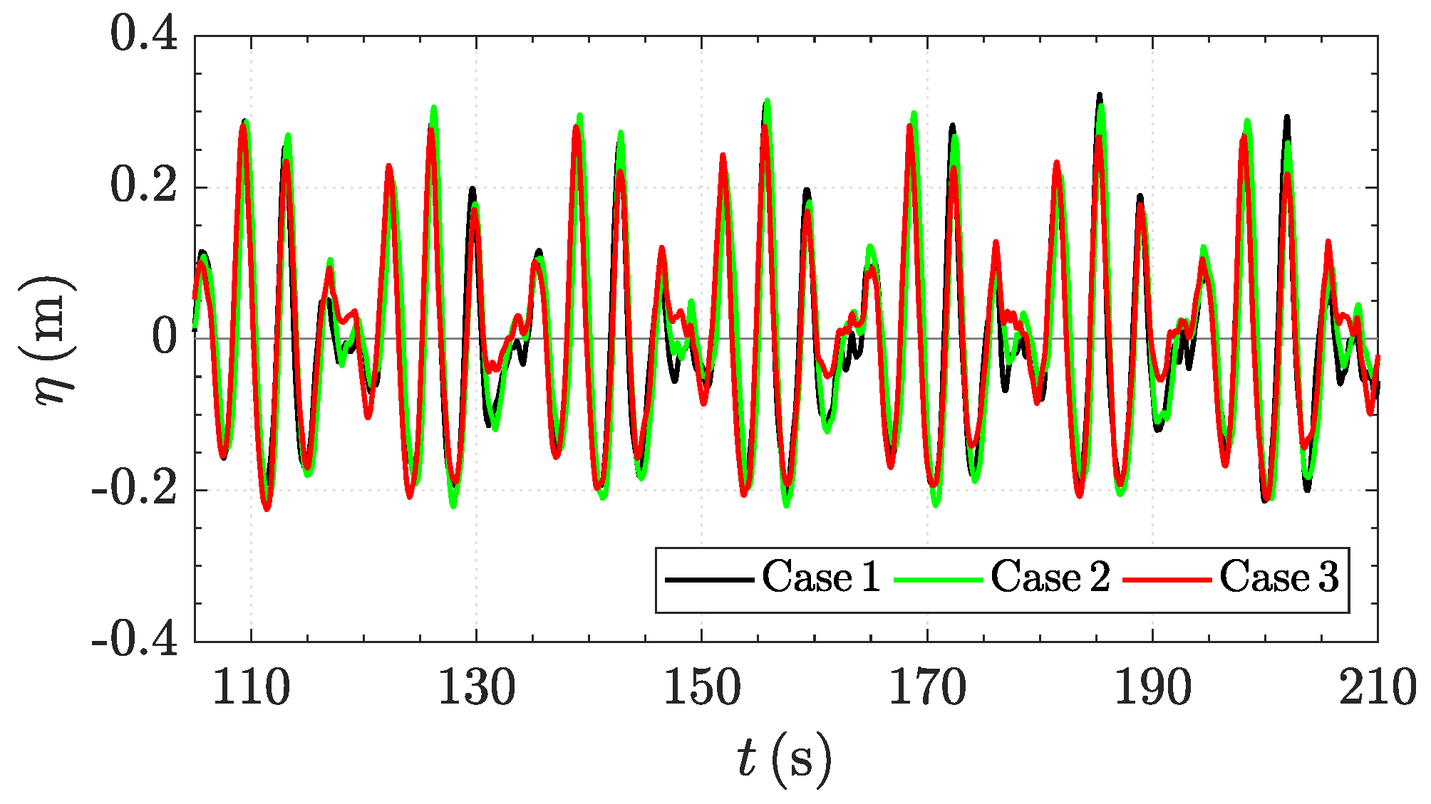
2.1. Wave Condition E2

Wave condition E2 is an energetic wave condition, which is typically classified as ‘erosive’ condition due to its comparably large dimensionless sediment settling velocity ($\mathsf{\Omega }$ = 3.9). It is a bichromatic wave condition which presents repeatable wave groups. In the RESIST project, repeatable wave conditions were required for the analysis of detailed sediment transport data which have been investigated in accompanying studies (see, for instance, van der Zanden et al. [29]). Previous studies on data from the same wave flume showed that beach profile evolution under bichromatic waves is similar to random waves, in contrast to monochromatic waves [30].

Details of the wave condition and its two components (with indices 1 and 2 for component 1 and 2, respectively) are summarised in

Table 2. Target values of wave condition E2.

${\mathbf{H}}_1$ (m)	${\mathbf{f}}_1$ (Hz)	${\mathbf{H}}_2$ (m)	${\mathbf{f}}_2$ (Hz)	${\mathbf{H}}_{\mathbf{s}}$ (m)	${\mathbf{T}}_{\mathbf{p}}$ (s)	${\mathbf{T}}_{\mathbf{g}}$ (s)	${\mathbf{T}}_{\mathbf{r}}$ (s)
0.245	0.3041	0.245	0.2365	0.49	3.7	14.8	29.6

. The target spectral wave height $H_s$ close to the wave paddle was 0.49 m and the mean primary wave period $T_p=2/(f_1+f_2)$ was 3.7 s. $T_g$ presents the period of one wave group ($T_g=1/(f_1-f_2)$), each comprising three short waves. $T_r$ corresponds to the repetition period, i.e., the period after which a defined number of wave groups repeats exactly. In the present case, $T_r=2·T_g$. The waves were fully modulated, i.e., $H_1=H_2$.

Waves were generated using first-order wave generation without active wave absorption to allow for sufficient stroke length to generate the high energy wave condition. Previous studies, which involved the same [21] and other data [31,32] from the same wave flume, described a minor influence (<1 cm) of basin seiching and other spurious long waves.

Each case of condition E2 consisted of four 30 min runs resulting in a total duration of 120 min of condition E2 in each case.

2.2. Measurements

The beach profile was measured along a central line of the flume after every 30 min run as well as before the start of condition E2. The profile measurements were performed by means of a mechanical profiler with a spacial resolution of 0.02 m and a vertical measuring accuracy of 0.01 m.

Information on the locations of the runup and rundown limit as well as on the offshore and onshore limit of wave breaking were acquired by means of visual observations during the first 5–10 min of each run. Wave breaking was identified visually as the point where the wave has started overturning (breaking point [33]) and before the collapsing wave hits the water surface (plunge point [34]). Owing to the bichromatic, i.e., repeatable, wave conditions, the breaking limits can be identified well by means of visual observation of a certain number of waves. Hence, the outer breaking location can be associated with breaking of the largest waves, the inner breaking location relates to breaking of the smallest waves of the group. The region offshore of the outer breaking location is hereafter defined as shoaling zone; the region onshore of the outer breaking is referred to as surf zone. The surf zone is further divided into the breaking zone, where most of the waves, large and small, break (region between outer and inner breaking), and the inner surf zone, where waves propagate as broken waves or turbulent bores (region onshore of the inner breaking up to the rundown limit) (adapted from [33,35]).

Water surface elevation was measured by means of resistive wave gauges (RWG) and acoustic wave gauges (AWG) at a frequency of 40 Hz. RWGs were primarily deployed in the deeper part of the flume and the shoaling region while AWGs were primarily deployed in the shoaling, surf and swash zones. In addition to water surface elevation, AWGs also measure exposed bed levels in the swash zone (see Section 3.3). In the inner surf and swash zone, i.e., between $x\approx$ −2 to 7 m, AWGs had a high spatial resolution of circa 1 m. The theoretical measuring accuracy of the AWGs is 0.2 mm, except for the two most onshore located AWGs for which it is 0.02 mm [29].

The three-dimensional velocity was measured at five fixed locations by means of acoustic doppler velocimeters (ADV) at a frequency of 100 Hz. The ADVs were deployed at a vertical elevation of 0.03 m above the initial bed and repositioned before the start of each run. An additional ADV was deployed at a mobile frame that is mounted to a mobile trolley allowing the horizontal and vertical positioning of the instrumentation.

In

Table 3. Instrument locations and vertical elevations above the bed at the start of the first run of case 1.

Device	Quantity	x-Location (in m) (vertical elevation above the bed (in m), where applicable)
RWG	12	−63.4, −48.22, −46.71, −42.3, −35.23, −31.16, −27.12, −23.18, −19.21, −17.42, −15.66, −11.3
AWG	19	−56.04, −44.94, −21.85, −20.55, −14.66, −13.26, −9.57, −7.38, −5.57, −3.44, −1.57, −0.52, 0.47, 1.25, 2.31, 3.5, 4.55, 5.56, 6.51
ADV	6	−11.39 (0.085), −1.54 (0.03), −0.52 (0.03), 0.27 (0.03), 1.28 (0.03), 2.26 (0.03)

, the instrument locations at the beginning of the first run of case 1 are summarised. For cases 2 and 3, the instrument locations were highly similar to case 1 with small variations between 2 and 20 cm in cross-shore direction which arise due to small variations in the handmade initial profiles of each sequence. In case 3, an additional ADV was deployed at x = −4.52 m at 3 cm above the initial bed.

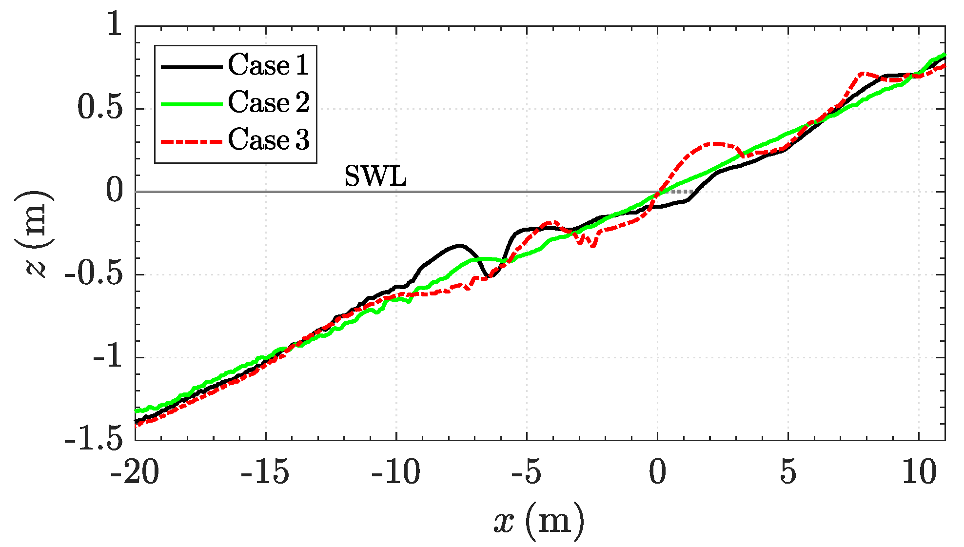
2.3. Initial Conditions

As aforementioned, condition E2 was performed three times but from varying initial morphologies. These morphologies are shown in Figure 1 and a brief description of the main features is given in

Table 4. Initial beach morphologies of the three cases.

Case	Overall Profile	Bar	Swash Berm
Case 1	Profile after slightly accretive condition	Offshore bar	Small swash berm
Case 2	(Almost) plane profile	Barless	No swash berm
Case 3	Low energy beach	Small bar in shallow water	Large berm with runnel

.

In case 1, condition E2 was run from a profile that developed under a (slightly) low energy condition with a dimensionless sediment settling velocity $\mathsf{\Omega }$ = 2. The resulting profile is characterised by a pronounced bar–trough relief (main breaker bar) with a secondary inner bar and a small berm (between $x\approx$ 2 to 3 m). This profile configuration can be classified following [9] as an intermediate beach with elements of the ‘rhythmic bar and beach state’ (RBB), such as a pronounced bar–trough relief and a small berm, even though three-dimensional features cannot be defined in the present study. It should be noted that the low energy condition prior to E2 was run from a high energy profile (see Table 1) after which limited shoreline recovery occured during the low energy condition [21]. Prior to the start of E2, the bar had a considerable volume, and it was located at $x\approx$ −7.7 m (Figure 1).

In case 2, condition E2 commenced from an almost plane, 1/15 sloped beach profile. Case 2 was run after 30 min of a random wave condition (condition B in Table 1) with $\mathsf{\Omega }$ = 3.09 (performed to homogenise and compact the manually shaped bed).

In case 3, the initial profile is a low energy beach with elements of a low energy intermediate ‘ridge-tunnel type’ (RR) and of a reflective beach [9]. Noticeable features of the initial profile are a small bar, a pronounced berm (at $x\approx$ 0 to 3 m) and a runnel. The profile had developed under a low energy wave condition with $\mathsf{\Omega }$ = 1.5 (see Table 1).

The initial shoreline location is relatively similar for cases 2 and 3 and is further offshore, i.e., the beach is wider, than for case 1. In both cases 1 and 3, the initial shoreline is found near the toe of the swash berm.

The same wave condition was performed in each case. Figure 2 shows a segment of circa 100 s of the water surface elevation measured at $x\approx$ −63.4 m (corresponding to circa 11.8 m distance from the wave paddle) which proves the similarity between the generated waves. The mean difference between the generated water surface time series lies between 0.1–1 % of the target $H_s$, which is in a similar range as the variability between the waves generated in different runs of E2 but within the same sequence.

3. Data Analysis

3.1. Sediment Transport Calculated from Bed Profile Measurements

Sediment transport rates $q({\mathrm{m}}^2/\mathrm{s})$ can be calculated at each cross-shore location $x_i$ (m) based on sediment mass conservation (‘Exner equation’) for any bed level change $\Delta z_i$ (m) over the associated time interval $\Delta t$ (s) [30]:

$$q\left(x_i\right)=q\left(x_{i-1}\right)-{\int }_{x_{i-1}}^{x_i}(1-p)\frac{\Delta z}{\Delta t}dx$$

(2)

where p (-) presents the porosity of the sediment which was previously measured and which is close to 0.4. q provides direct indication of the direction and magnitude of sediment transported along the profile. This calculation is performed starting from the offshore or onshore boundary ($x_{off}$ and $x_{on}$, respectively) beyond which no sediment transport occurs (closure limits). Positive values of q indicate onshore sediment transport; negative values correspond to offshore sediment transport.

Integration of q along x and multiplication by the time interval $\Delta t$ between the profile measurements yields the bulk sediment transport $Q\left({\mathrm{m}}^3\right)$ [30]:

$$Q=\Delta t{\int }_{x_{off}}^{x_{on}}q\left(x\right)dx$$

(3)

Q provides an indication of the overall beach response being erosive (negative values of Q) or accretive (positive values of Q).

3.2. Data Treatment

ADVs were primarily placed in the inner surf and swash zone where the sensors are intermittently emerged and submerged. Low quality data, primarily associated with exposed sensors during wave backwash, were detected based on correlation statistics (signal amplitude below 75 counts or signal-to-noise ratio below 15 dB), discarded and not replaced. From the cleaned data, spurious high frequency data are removed by applying a low-pass filter with a cut-off frequency of 3 Hz. The first 60 s and the last 120 s of each ADV time series were discarded.

The repeatable bichromatic wave conditions allow ensemble averaging of hydrodynamic measurements at the repetition period. The detailed procedure to obtain the ensemble averaged data are described in van der Zanden et al. [29]. Subsequently, the maximum wave height $H_{max}$ is obtained as the difference between the maximum and the minimum water surface elevation of an ensemble.

3.3. Bed Level Changes from AWG Measurements

AWG measurements in the inner surf and swash zone can be used to obtain bed level changes [29,36,37]. AWGs measure the distance to the surface and are calibrated to an initial level, which is, depending on their cross-shore location, either the still water level or the exposed bed. When waves run up and down the beachface between the locations of the rundown and runup limit, the bed is intermittently exposed, which is also measured by the AWGs.

Based on the rundown limit, which was observed during the experimental run, and visual inspection of the AWG time series, the most offshore AWG location where the bed was intermittently exposed and hence, measured by the AWGs, was identified. Because some AWGs have their initial reference with respect to the still water level and to ensure the first short waves have arrived at the beach, the initial bed level is taken as the exposed bed after circa 90 s (after the first three wave groups). Subsequently, a moving minimum approach is applied with a window size corresponding to the repetition period ($T_r$ = 29.6 s) to obtain bed level changes between consecutive wave group repeats.

4. Results

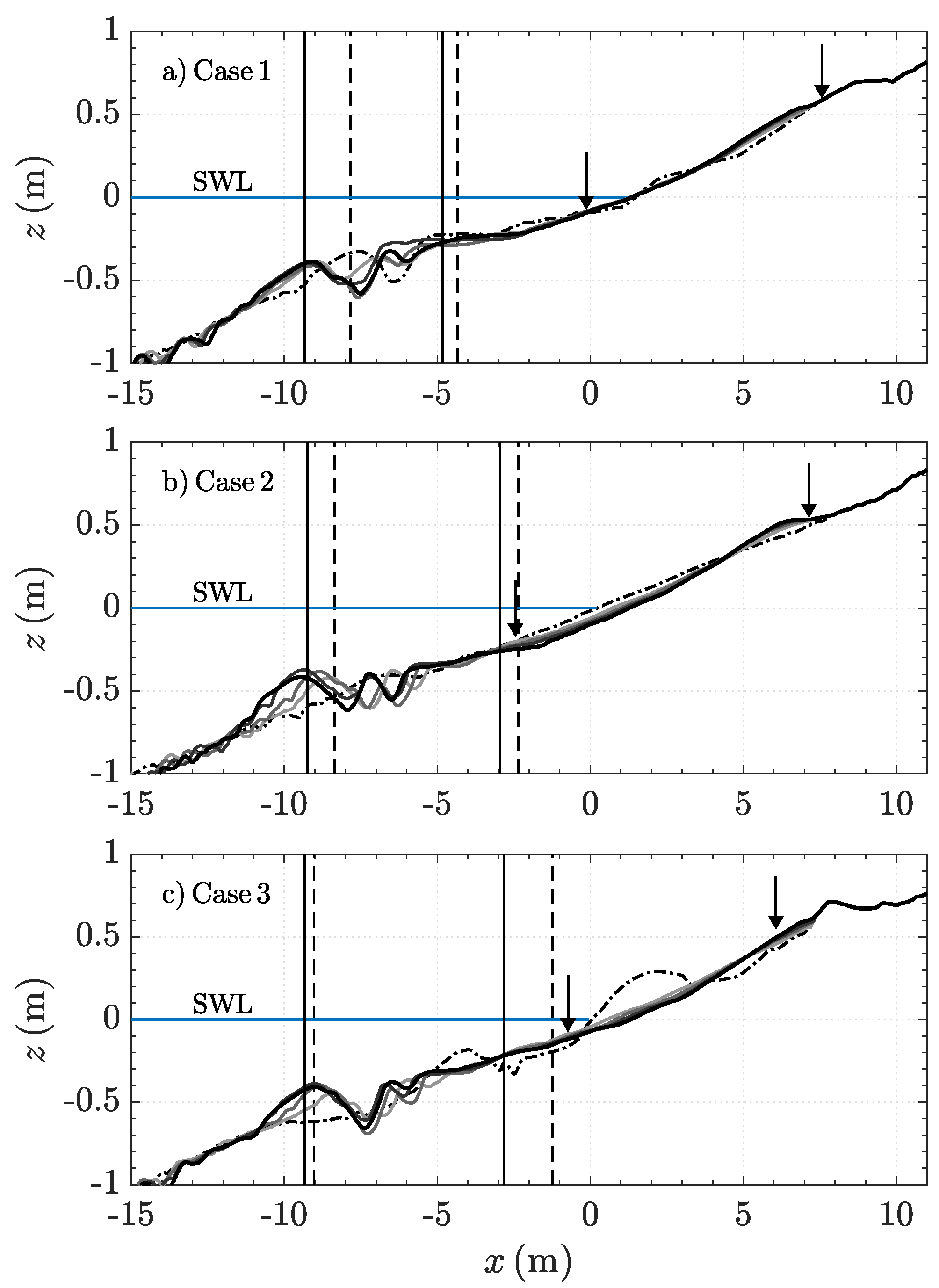
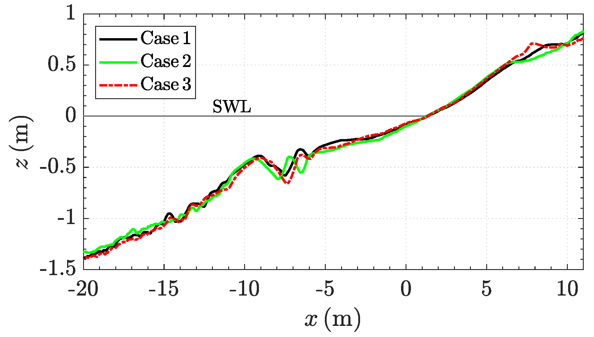
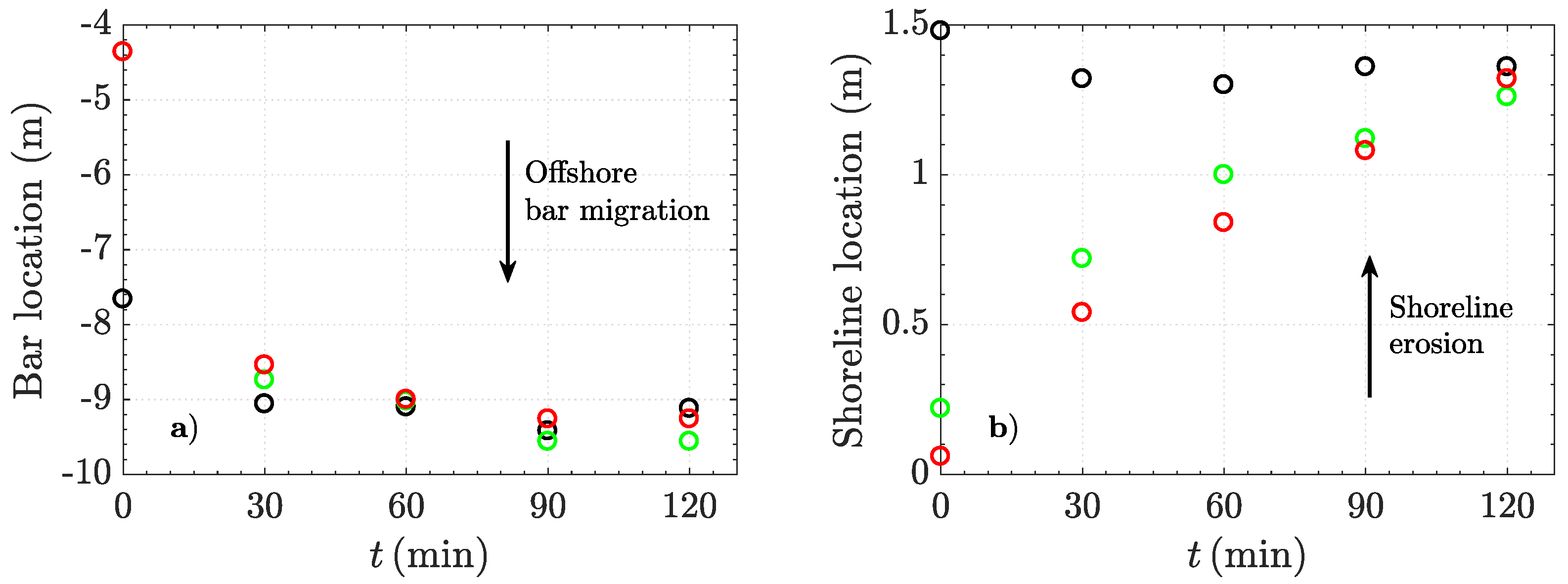
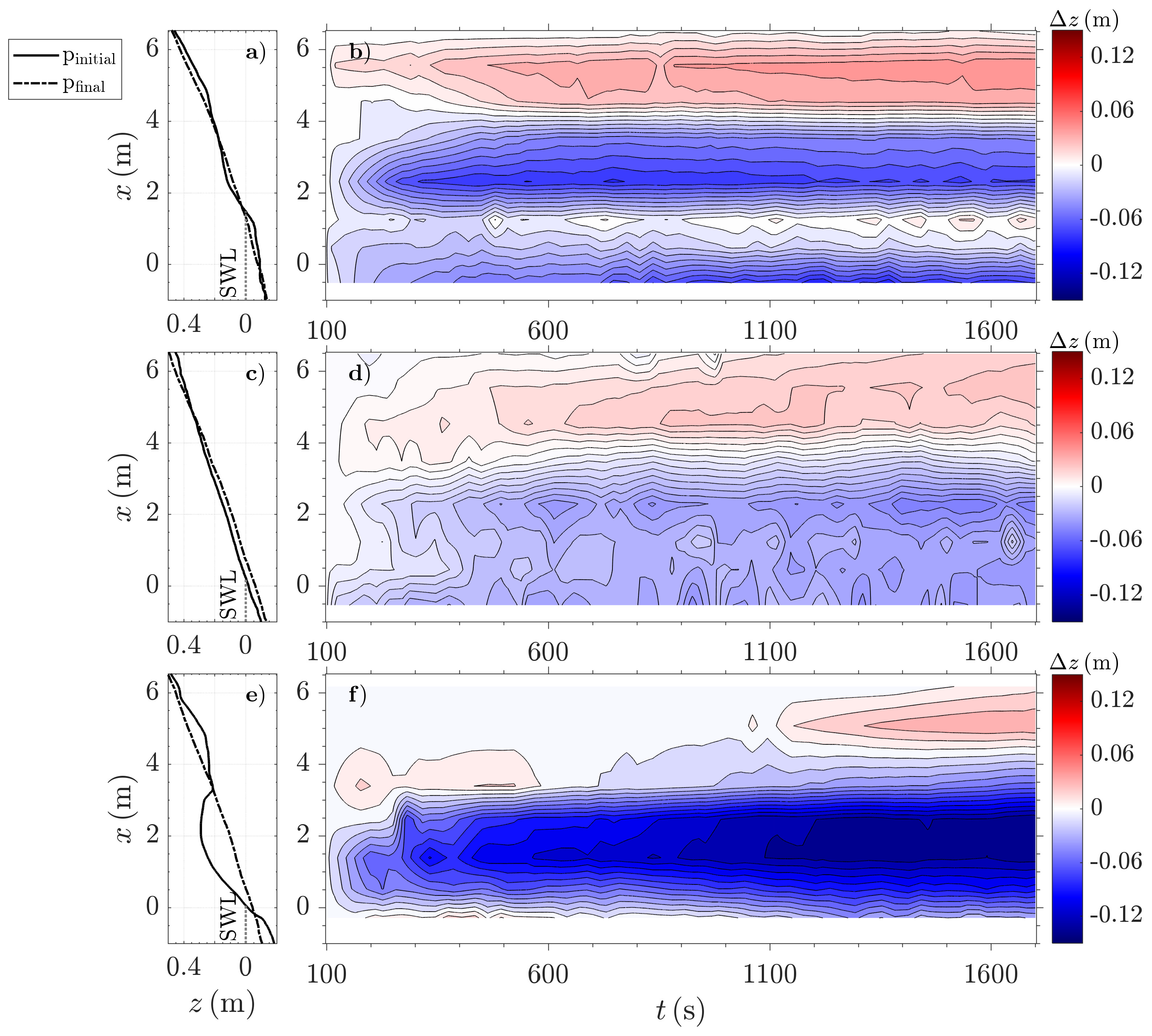
4.1. Profile Evolution

The beach profiles obtained by means of the mechanical profiler in intervals of 30 min (after each run) are shown in Figure 3 for cases 1–3 (panels a–c, respectively). The colour changes from light to dark as time progresses. The final profiles of the three cases are shown in Figure 4.

It becomes evident that the beach profile develops towards a similar final profile in the three cases (Figure 4 and black lines in Figure 3), characterised by a main breaker bar–trough system and a secondary bar, a concave profile in the inner surf and swash zone, and the presence of a small berm at the maximum runup location. This final beach configuration is considered to be the equilibrium profile associated with condition E2. The same final beach profile develops, even though the cases start from highly different initial morphologies, indicating that the final profile configuration is largely determined by the wave condition (in line with e.g., [4,7,19,21]).

Largest beach changes occur during the initial stage of condition E2 and beach changes become smaller as the profile approaches the final (equilibrium) configuration (Figure 3). Case 1 (intermediate initial beach profile) is characterised by offshore migration of the breaker bar and of the outer breaking location (from $x\approx$ −7.7 m to $x\approx$ −9.1 m), including also offshore migration of the secondary inner bar and the inner breaking location. The small existing berm (at $x\approx$ 2.5 m) disappears and a new berm evolves close to the maximum runup location. In case 2 (almost plane 1/15 sloped initial profile), a breaker bar develops at $x\approx$ −8.7 m and shows only little offshore migration to $x\approx$ −9.5 m towards the final beach configuration. The shoreline erodes and a berm forms near the maximum runup location as the beach evolves from a planar to a concave profile. In case 3 (low energy initial profile), the existing bar (at $x\approx$ −4.4 m) is eroded and a new bar forms further offshore near the bar location of the final beach configuration (at $x\approx$ −9.3 m). The large berm of the initial profile is eroded along with the shoreline. As in cases 1 and 2, a small berm evolves near the maximum runup limit.

A fast evolution of the beach during the initial stage of a wave condition are in line with equilibrium-type beach evolution models, which state that beach changes are faster for a larger disequilibrium of the beach profile for a given wave condition [4,7]. In addition, beach changes in the beginning of relatively energetic wave conditions, such as the present condition E2, were previously reported to occur quickly [21,27].

During the first run, differences in the wave breaking location (vertical dashed lines in Figure 3) highlight the morphodynamic feedback. In case 1, the outer breaking location is controlled by the offshore located bar that is present at the beginning of condition E2. In contrast, in cases 2 and 3, the outer wave breaking location is initially not controlled by the breaker bar. This is because the initial profile is an almost plane profile (case 2) or the bar is small and far onshore so that the largest waves break before arriving at the existing bar location (case 3). In these cases, the outer wave breaking occurs close to the final bar location of condition E2 where the bar is located directly after the first wave run. Generally, the breaker bar is found near the outer breaking location similar to other wave conditions in the same experiment [21] and in other studies, especially for high energy wave conditions [11,12,13,38,39]. Towards the end of condition E2, the outer wave breaking location (last run indicated by vertical solid lines) is highly similar between the cases. This indicates the importance of the coupling between morphology and hydrodynamics during the first run leading to the equilibrium profile.

Differences between the cases can also be observed in terms of the region between the rundown and runup limits, i.e., the swash excursion. The swash excursion appears to be largest in case 2, which started from the almost plane beach profile. Due to the plane profile, there were no beach features that hindered the waves from going up onto the beach and running back. In case 3, the wave runup goes beyond the berm directly from the beginning of condition E2, which is important for the evolution of the swash berm as will be further shown in Section 4.5.

The evolution of the different initial beach profiles towards the same final (equilibrium) morphology is also supported by the similarity of specific beach parameters, such as the bar and the shoreline location (Figure 5). Figure 5 reveals an equilibrium bar location at $x\approx$ −9.3 m and an equilibrium shoreline location at $x\approx$ 1.3 m with a variability between the cases of 0.44 m and 0.1 m for the bar and the shoreline, respectively, which can be considered small [13]. The final equilibrium shoreline and bar locations are the same despite the differences in the initial locations. The disequilibrium of the bar and the shoreline in the beginning of condition E2 is largest in case 3 and smallest in case 1.

The bar reaches its equilibrium location during the first run of condition E2 (Figure 5a). As aforementioned, the bar of the initial profile of case 3 does not migrate offshore but is eroded and a new bar forms during the first run of E2 in case 3.

Differences in beach evolution between the three cases become also evident for the shoreline (Figure 5b). While the shoreline erodes in cases 2 and 3, it is at a relatively stable location in case 1. This can be related to the initial shoreline in case 1 being close to the equilibrium shoreline location of condition E2. In both case 1 and case 3, the initial shoreline is at the toe of the swash berm. In case 1, this berm is small and hence does not have an important effect on the shoreline location after being eroded, while, in case 3, the berm is large and, hence, strong erosion of the berm leads to a large shift of the shoreline towards the onshore.

It becomes evident that largest morphological changes occur during the first 30 min of condition E2. Therefore, we will primarily focus on this run in what follows.

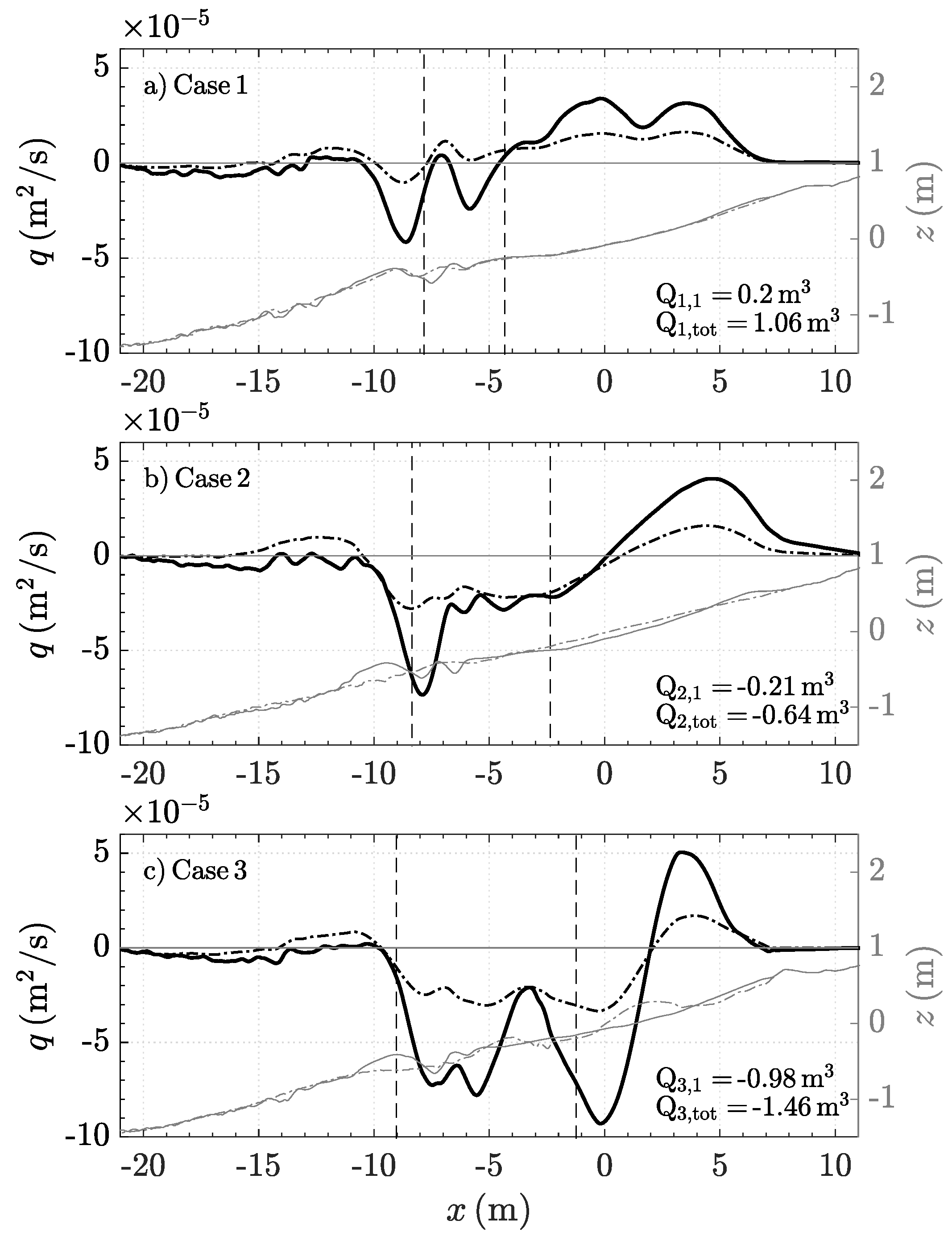
4.2. Sediment Transport

Sediment transport rates q can be calculated from bed level changes following Equation (2). Figure 6 shows q along the flume during the first run of E2 (solid lines) as well as q over the entire 120 min duration of condition E2 for reference (dashed-dotted lines). Note that q presents a time-averaged quantity over the duration $\Delta t$ (see Equation (2)) and, therefore, q over the entire 120 min duration can have smaller magnitudes than q during the first run.

Some similitude in the cross-shore shape for both q during the first run as well as for q during the entire duration of E2 can be observed: (1) Slight onshore sediment transport in the shoaling region before wave breaking which is usually associated with wave asymmetries [10,11,40,41,42]. (2) Offshore sediment transport around the breaking zone, typically associated with offshore directed mean return flow (undertow) [10,11,12,42]. A wider breaking zone corresponds to a wider region of offshore sediment transport in Figure 6 (compare, for instance, case 1 and case 3). It can be noted that the observed limits of the breaking zone do not always perfectly coincide with the separation between on- and offshore sediment transport which might be related to limitations in the visually observed breaking locations as well as the driving processes acting slightly beyond the observed breaking limits. (3) Positive sediment transport in the most onshore part of the swash zone (i.e., $x>$ 2 m) resulting in filling of a previously formed runnel and/or building of a berm [15,18,43]. This berm is smaller and located further onshore than the swash berm of the initial profile (at $x\approx$ 6–7 m).

A closer examination of the three cases reveals differences between the sediment transport rates of the three cases. Maximum offshore sediment tranport magnitudes are larger in cases 2 and 3 compared to case 1 and, as aforementioned, offshore transport occurs over a wider region associated with a wider breaking zone. This can be related to the evolution of the breaker bar: while the size and shape of the bar in case 1 does not change significantly and, hence, does not require additional sediment supply, the bar in cases 2 and 3 forms during the first run of E2. In addition, in case 3, the small initial onshore located bar gets eroded resulting in large sediment transport magnitudes at $x\approx$ −5 m.

In the inner surf and the most offshore region of the swash zone sediment transport magnitudes and directions are highly different between the cases, especially between cases 1 and 3. In case 1, the sediment in the inner surf zone is moved onshore to build the new berm at $x\approx$ 6 m. In contrast, in case 3, large offshore sediment transport magnitudes are present in the inner surf zone which sharply change into onshore directed sediment transport at $x\approx$ 2 m. Combining this with the initial beach profile of case 3, it appears that sediment onshore of the crest of the berm, i.e., $x>$ 2 m, is moved onshore filling up the runnel, while sediment offshore of the berm crest is moved offshore filling up the trough of the initial bar and supplying sediment towards the formation of the newly developing bar.

In terms of sediment exchange between the surf and the swash zone, the above observations indicate that, in case of a low energy initial profile (case 3), a large amount of sediment is drawn from the swash into the surf zone as the berm gets eroded. In contrast, in case of the intermediate energy initial profile (case 1), sediment is moved from the surf into the swash zone.

Overall, the identified differences in sediment transport rates result in different values of the bulk sediment transport Q between the cases. $Q_{tot}$ can also be considered as a quantification of the disequilibrium of the initial beach profile to its final configuration, i.e., how much bulk sediment needs to be moved for the profile to reach its equilibrium for the prevailing wave condition. For the present study, where all cases result in a similar final profile, case 1 (intermediate energy initial profile) requires a positive (onshore) bulk sediment transport to reach the final profile configuration. In contrast, for the initial plane and low energy profile in cases 2 and 3, respectively, negative (offshore), bulk transport is needed to reach the final profile that is more eroded compared to the initial profiles. Negative Q values are largest in case 3 indicating a large disequilibrium of the initial beach morphology.

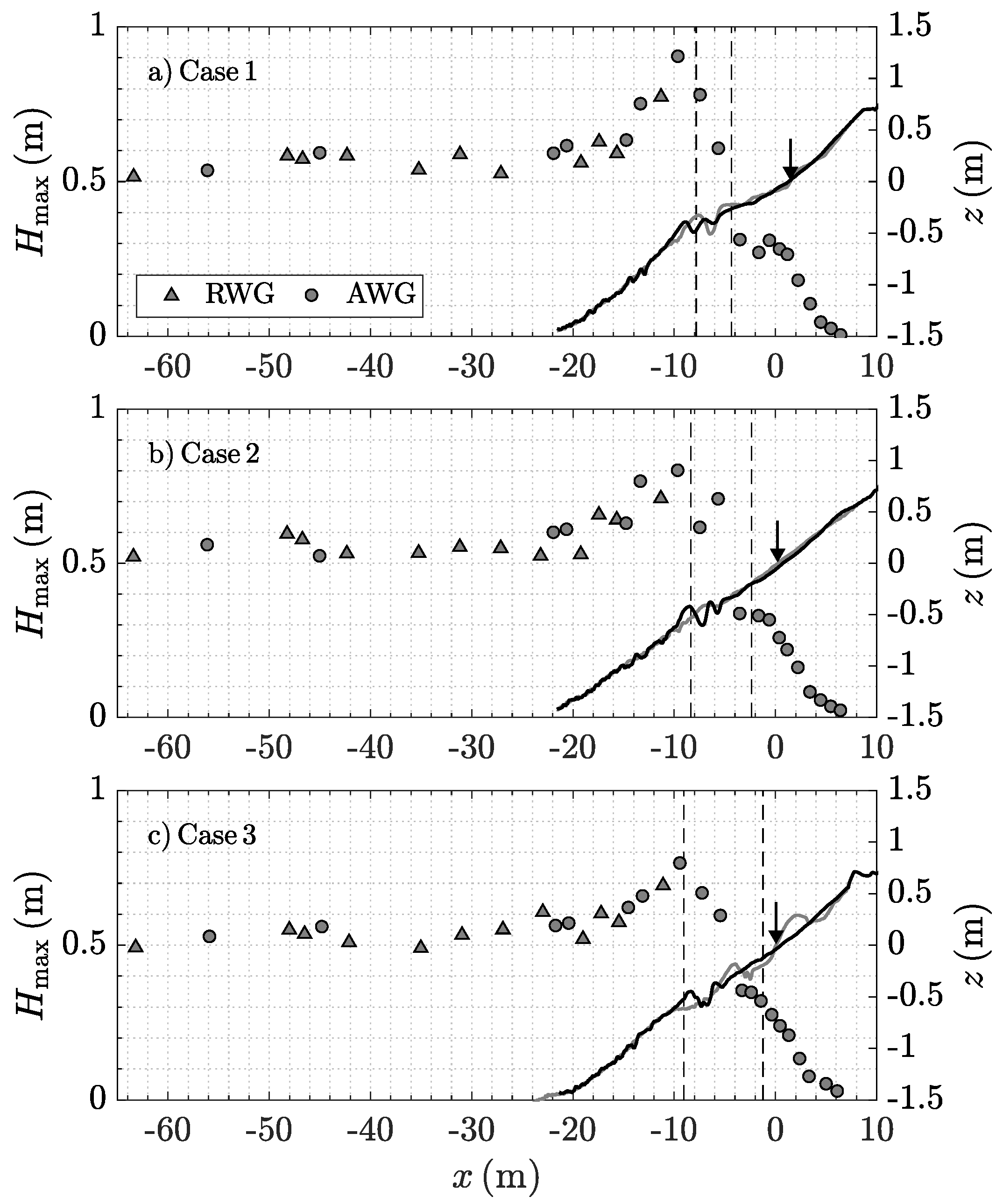
4.3. Wave Heights along the Flume

The water surface elevation was measured at a high spatial resolution along the flume allowing the investigation of the cross-shore wave height evolution. Figure 7 presents the wave height during the first run of E2 along the flume measured by means of RWGs and AWGs (left ordinate). The wave height is presented as maximum wave height $H_{max}$ of the ensemble averaged data of the first run. $H_{max}$ accounts for all waves in each ensemble and, therefore, presents a useful indicator for the wave height reduction and, hence, energy dissipation of the entire repeatable wave train. The profiles before and after the run as well as the breaking zone are also shown for reference.

A typical cross-shore pattern of wave height evolution can be observed with relatively constant wave heights in the planar bed part of the flume, increase of the wave height due to shoaling when waves get into shallower water and subsequent wave height reduction and associated energy dissipation due to wave breaking. In all three cases, largest values of $H_{max}$ occur at the outer breaking location associated with large instability of the shoaling waves.

Some differences in the cross-shore wave height evolution between the three cases can be observed even though Figure 7 suggests that these differences are relatively small between the cases, especially compared to the large differences in sediment transport rates (Figure 6). Evident differences occur primarily in the breaking zone and can be linked to the differences in the initial profiles. As mentioned in Section 4.1 and as also evident from Figure 7, wave breaking initiates more onshore in case 1 compared to cases 2 and 3 as it is controlled by the initial bar. Moreover, maximum values of $H_{max}$ at the outer breaking location are largest in case 1, which can be associated with the steep offshore slope of the bar promoting wave shoaling. Subsequently, the bar promotes breaking of all, including the smallest, waves resulting in a narrow breaking zone associated with concentrated wave energy dissipation. In this region, a strong mean return flow [10,11,12] and high suspended sediment concentrations due to breaking-induced turbulence [42] may exist, moving the existing bar offshore. The confined region of wave energy dissipation links up with the narrow region of offshore sediment transport in case 1, as was shown in Figure 6a.

Consequently, the existing bar in case 1 and the associated larger energy dissipation importantly contribute to the protection of the beach from the incoming waves. Waves of large wave height or breaking waves may not get as close onto the beach protecting the beach from the wave impact. This is in line with, for instance, Grasso et al. [24], who reported that a larger bar promoted increased wave energy dissipation resulting in less offshore sediment transport and reduced shore erosion.

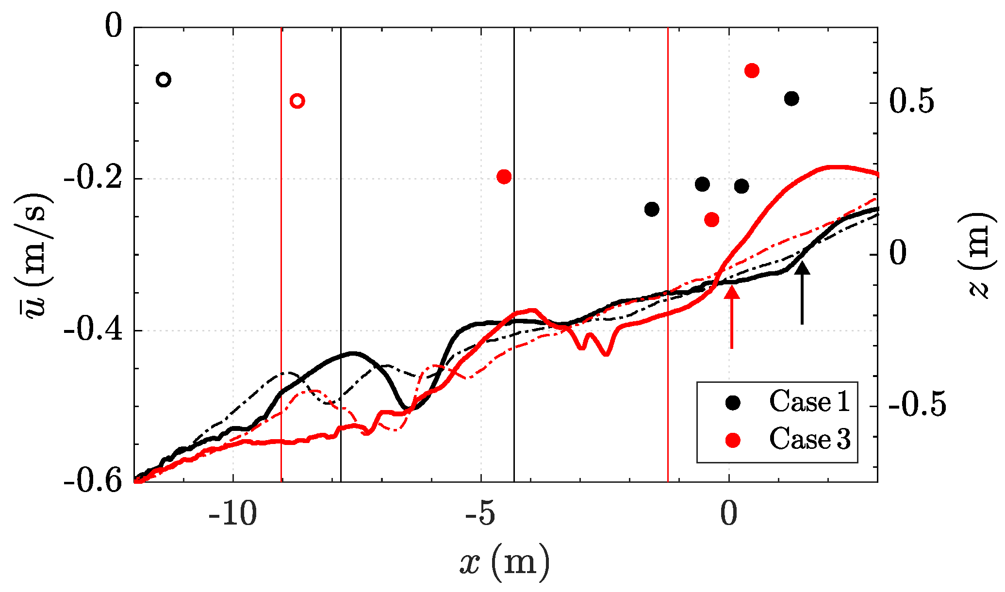
4.4. Time-Averaged Velocities

Figure 8 shows the time-averaged near-bed flow velocities $\overline{u}$ (Figure 8) in the inner surf and swash zone. For case 2, the velocity measurements could not be included due to limited data quality. From the second run, the mean velocities were found to have a highly similar cross-shore shape and magnitude between the three cases which highlights that a morphodynamic feedback exists, i.e., differences between the mean velocities of cases 1 and 3 during the first run can be linked to the differences in the initial profiles.

A general cross-shore shape of the mean velocities, which are all offshore directed, becomes evident from Figure 8: mean velocities have small magnitudes offshore of the breaking zone which is associated with limited offshore sediment transport (see Figure 6a,c). Note that these velocities were measured at 8 cm in case 1 and at 10 cm in case 3 from the initial bed and hence, velocities measured closer to the bed would be expected to be of even smaller magnitude. Mean velocities become more negative towards the onshore and have their largest magnitude onshore of the breaking zone which may, however, be related to the measuring resolution. Mean velocity magnitudes decrease onshore of $x\approx$ −1 m.

The spatial resolution of the velocity measurements is limited in the breaking zone and, hence, does not allow for a clear link between the mean return flow and the breaker bar evolution as well as the investigation of the differences between case 1 and case 3 from the data. In case 1, offshore directed mean velocities would be expected to have a maximum in the breaker zone in line with previous studies [10,11,42]. This is also where largest offshore sediment transport takes place contributing to the offshore migration of the breaker bar (see Figure 6a).

Around $x\approx$ 0 m, i.e., in the inner surf and the beginning of the swash zone, the spatial measuring resolution is larger and Figure 8 indicates differences between the two cases. In case 3, a strong reduction of the mean velocity magnitude occurs over a narrow cross-shore region (two red dots at $x\approx$ −0.5 m and 0.5 m). In contrast, in case 1, the decrease of the the velocity magnitude appears to be more gentle and the velocity magnitude is closer to zero at the initial shoreline (see arrows in Figure 8). These differences can be related to differences in the berm between the two cases where the berm is much larger and steeper in case 3. In fact, the reduction of the mean velocity in case 3 occurs almost exactly over the steep offshore-facing berm slope which has similarly been observed in the field [43]. Consequently, the large and steep berm decelerates the mean flow velocity towards its crest and increases it towards the toe. Since this happens over a narrow area due to the large slope of the berm, this change in velocity is associated with a large gradient in sediment transport rate (see Figure 6c) mobilising an important amount of sediment at the toe of the berm where large offshore mean velocities coincide with largest offshore sediment transport magnitudes.

In contrast, in case 1, the berm is much smaller, and the velocity reduces more gently. The velocity magnitude is smallest near the toe of the berm, which corresponds to the location of the initial shoreline of case 1. This might be related to the onshore limit of the breaking zone being further offshore as it does not allow unbroken waves to get close onto the beach compared to case 3. This again highlights the importance of the breaker bar promoting wave breaking and hence wave energy dissipation further offshore. The smaller mean velocity magnitudes at the initial shoreline in case 1 are less likely to promote erosion; in fact, Figure 6a suggests onshore sediment transport in this area. Berm formation and onshore sediment transport in the swash zone have been linked to the advection of sediment from the inner surf and/or lower swash zone, even under conditions with negative mean near-bed velocities [17,18].

4.5. Bed Level Changes during the First Run in the Swash Zone

Bed profile measurements were performed between each wave run and hence provide information on bed level changes with a temporal resolution of 30 min. As shown in Section 4.1, largest morphological changes occur during the first run of condition E2. To investigate the bed evolution within this first run in further detail, the bed profile change in the inner surf and swash zone obtained by means of the AWG measurements (as described in Section 3) is shown in Figure 9 (right panels). For reference, the left panels show the corresponding initial and final profile of the first run obtained by means of the mechanical profiler.

Observations can be made in terms of the timing of the evolution towards a concave swash profile and associated differences in the evolution between the cases. In case 1, both erosion of the berm and onshore deposition of sediment (at $x>$ 4 m) start from the beginning of the run. At the initial shoreline location ($x\approx$ 1.5 m), the profile change is very small with small accretion towards the end of the run which is in line with the slight shoreline accretion (see Figure 5b). Overall, the volume of the sediment deposited onshore of $x>$ 4 m is larger than the eroded volume resulting in overall onshore directed sediment transport in this area (see Figure 6a and Figure 9a,b).

In case 2, which started from the plane profile, no beach features are present and a clear separation (at $x\approx$ 3.5 m) between an area of sediment deposition ($x>$ 3.5 m) and erosion ($x<$ 3.5 m) can be observed towards the evolution of a concave swash profile, which is supported by previous studies [18,29,44]. The net transport of sediment is negative resulting in a net export of sediment from the swash to the inner surf zone (see, for instance, van der Zanden et al. [29]). Sediment deposition initiates almost at the same time as sediment erosion. In both case 1 and case 2, largest morphological changes occur within the first 600 s of condition E2.

Case 3 commenced from the profile with the large berm, which constitutes a more complex case in terms of the temporal evolution of the swash zone in the form of a step-wise evolution. The erosion of the berm starts from the beginning of the run due to the large runup. Initially, overwash over the initial berm transports sediment onshore into the runnel (at $x>$ 3 m). The overwash occurs because the wave runup (at least of the largest waves of the groups) from the beginning of the run is sufficiently large to pass the berm (see Figure 3c). The overwash does not directly flow back and hence sediment is deposited. At the same time, erosion at the offshore slope of the berm occurs due to the backwash from which sediment is deposited in the inner surf zone. These processes reduce the height of the berm crest (at $x\approx$ 1.5 m), subsequently allowing also smaller waves to pass the berm. This results in further erosion of the berm between circa 600–1000 s of this run without further deposition of sediment onshore. Only when the berm is almost fully eroded, the runnel onshore of the initial berm continues to fill up. This detailed berm destruction by overwash measured in the present laboratory experiments is similar to the beach scarp destruction described under natural conditions by Ruiz de Alegría-Arzaburu et al. [45] and Bonte and Levoy [46].

The described pattern suggests that, in case 3, first, the berm height needs to reduce resulting in a profile that is considered similar to the initial profile of case 1. Subsequently, the evolution pattern is similar to case 1 onshore of $x\approx$ 4 m. Consequently, the swash evolution towards the concave (storm) profile in case 3 appears to be temporally delayed compared to case 1 due to the large, initial berm in case 3, which is fully eroded after circa 1000 s.

For all three cases, the bed evolution in the swash zone is the result of a sediment redistribution within the swash and a net exchange of sediment with the inner surf zone. Case 1 leads to net import of sediment into the swash zone, while cases 2 and 3 induce net export of sediment from the swash into the inner surf zone.

5. Conceptual Model and Discussion

The different initial beach morphologies evolve towards the same final equilibrium profile. Differences in the beach evolution are linked to differences in the coupling between beach morphology and hydrodynamics in the three cases. The findings of the present study are, to some extent, also related to the experimental conditions of medium sediment size, a relatively steep beach slope (average slope of 1/15), and moderate wave energy conditions where the same wave condition that started from different initial morphologies generates the same final beach configuration. Other studies, for instance Birrien et al. [20], reported that the initial morphology can also have an effect on the final beach configuration.

It needs to be noted that only the largest differences in hydrodyamics between the three cases could be linked to the initial morphologies because most of the variability in the hydrodynamics between the cases was small, especially compared to the large morphological changes. Analysis of hydrodynamic data at an intrawave scale did not provide evidence of differences between cases to be larger than the variability within one case which highlights limits of the measuring accuracy. Therefore, the analysis focused on quantities averaged over the first run. Time-averaged quantities were found to converge between cases for the subsequent runs highlighting the influence of the initial morphology on the first run. The differences in hydrodynamics between the cases being small is related to the fact that the generated waves are highly similar (Figure 2) and the differences only result from different morphologies and its coupling to the hydrodynamics. An additional measuring limitation is related to the spatial resolution of velocity measurements which were primarily acquired in the region around the shoreline.

Despite these limitations, clear effects of the different initial beach morphologies on equilibrium beach evolution have been identified in the present study. The core findings are summarised in a conceptual model that is shown in Figure 10. Two different initial morphologies are presented in Figure 10a,b, similar to case 1 and case 3, respectively, which were subjected to the same incident wave conditions. The conceptual model has elements of the equilibrium beach state model of Wright et al. [4] even though the present work does not primarily look into changes between beach states but rather focuses on the processes involved in equilibrium beach evolution.

In the case of an intermediate energy initial profile (Figure 10a), $\mathsf{\Omega }$ of the incident wave condition is slightly larger than the ${\mathsf{\Omega }}_0$ under which the initial beach profile evolved. The existing bar plays an important role for the equilibrium evolution as it promotes wave breaking and, hence, has a sheltering effect for the beach. Wave breaking at the bar results in fast wave height reduction and associated energy dissipation of all waves around the bar region with offshore sediment transport and largest offshore mean velocity magnitudes at around the onshore limit of the breaking zone. This drives the existing breaker bar offshore towards the equilibrium bar location of the (energetic) wave condition. Changes in the bar shape and volume are limited, and only small additional sediment volumes are drawn from around the breaking zone. Small, broken waves arrive at the shoreline where offshore mean velocities are small and reduce gently over the existing, small berm. As a result, sediment transport is onshore directed in this part of the beach where shoreline changes are limited and the sediment of the small swash berm is moved onshore to form a concave, featureless swash profile.

In the case of a lower energy initial profile (Figure 10b), the wave energy disequilibrium is large ($\mathsf{\Omega }\gg {\mathsf{\Omega }}_0$), promoting fast beach evolution towards a more dissipative state [4,7]. The existing breaker bar in shallow water becomes inactive when the higher energy wave condition starts. Outer breaking occurs at the location where the new breaker bar forms, i.e., at the new equilibrium bar location. The smaller waves of the group break close to the shoreline resulting in a wider breaking zone and associated energy dissipation. This promotes offshore sediment transport in the wider breaking zone which contributes to the generation of the new breaker bar further offshore. The swash berm is an important feature of the low energy beach. Mean flow velocities are small at the berm crest and the flow accelerates towards the toe of the berm, promoting erosion close to the initial shoreline. Initial overwash presents an important process that initiates the decay of the berm.

An important aspect of the two distinct ways of beach evolution is that bulk sediment transport is onshore directed in case 1 but offshore directed in case 3 (Figure 6 and Figure 10). This highlights that the same wave condition, which is classified as a high energy condition and which would, therefore, traditionally be expected to erode the beach, can produce either onshore or offshore sediment transport depending on the initial morphology [7,21]. In the present study, sediment is transported onshore in the inner surf and swash zone in case 1. This is related to specific conditions in comparison to case 3 that can promote onshore sediment transport, which are the narrow breaking zone which is confined around the breaker bar, and the weaker and more gently reducing mean offshore velocities in the inner surf and swash zone. Onshore sediment transport despite offshore mean velocities was observed in previous studies which similarly linked it to weak mean currents that are not strong enough to promote offshore transport leading to a dominance of the onshore-directed wave-related transport [43].

The present study also highlights the importance of the bar and the berm as beach features, each of them functioning in a way to protect the beach against the wave impact. An existing, active breaker bar promotes wave energy dissipation and migrates offshore. This does not require much additional sediment from the inner surf and swash zone, which limits morphological changes in this region.

In case of a low energy profile, the berm presents an important protection against storm events as it presents a large sediment volume that is eroded before further sediment is drawn from the inner surf and swash zone. Previous studies similarly stated that a more recovered beach has a larger volume of sediment that can be eroded initially [7,22,26]. This results in a temporal delay of the inner surf and swash zone to arrive at its more eroded, equilibrium profile. However, the beach is generally considered to evolve fast under energetic wave conditions [21,27,39] and hence the temporal delay has to be considered as a temporally limited protection against wave impact. It would be of interest to investigate further to what extent the size of the berm affects erosion in the inner surf and swash zone. In the present study, initial overwash and resulting onshore sediment transport initiate the destruction of the berm. In case of a larger berm, the run-up of the present wave condition may not go beyond the berm from the beginning of the condition and hence initial berm erosion would be limited to the offshore side of the berm. Other processes, such as strong erosion of the offshore side of the berm or infiltration, may be of importance.

6. Conclusions

The same wave condition was run from three different initial beach morphologies in a large-scale wave flume and resulted in a similar quasi-equilibrium beach profile. The three initial morphologies were an intermediate energy profile, a plane profile and a low energy profile. Beach profile and hydrodynamic measurements, as well as calculations of sediment transport and bed level changes, were studied to explore the role of differences in the initial morphology on beach profile evolution towards equilibrium.

The results lead to the following conclusions:

• The beach evolves towards the same final (equilibrium) morphology that is determined by the wave condition. Different initial beach morphologies do not alter this equilibrium beach morphology but produce different sediment transport patterns, associated with differences in the hydrodynamics, to reach the equilibrium morphology.
• Differences in the profile morphology and hydrodynamics are largest during the first 30 min run, highlighting an important coupling between the beach morphology and the hydrodynamics. When the beach profile is more stable (from the second wave run), the hydrodynamic differences that arise from the different beach morphologies, diminish and more detailed measurements would be needed to investigate effects of morphodynamic coupling on equilibrium beach evolution on a more detailed scale.
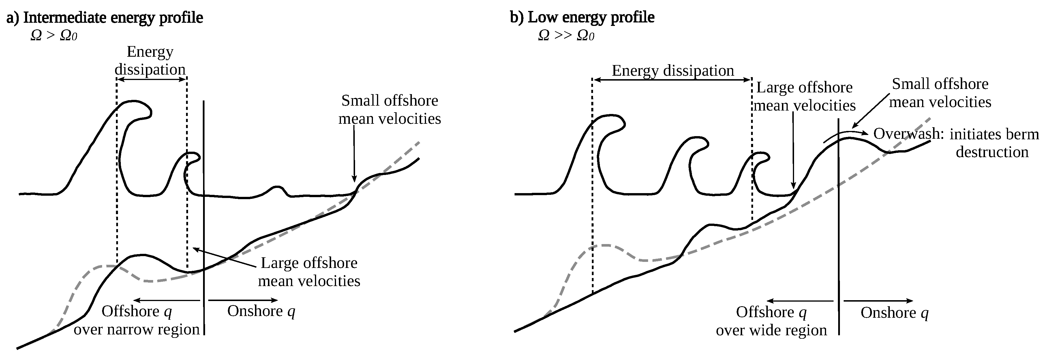
• The bar of the initial profile—and, more specifically, its size and location—presents an important morphological feature for the equilibrium beach evolution. The size and location of the bar determine if the bar controls the wave breaking location and associated wave energy dissipation. In case of an intermediate energy profile with an existing breaker bar, wave energy dissipation is confined around the bar in a narrow zone leading to offshore sediment transport in this region and providing a sheltering effect for the inner surf and swash zone. In case of a low energy profile, the initial bar does not control the wave breaking location and wave energy dissipation occurs over a wider cross-shore region associated with offshore sediment transport.
• The large swash berm of the initial low energy profile plays an important role for the equilibrium beach evolution. The berm presents a large source of sediment which is partly moved onshore to fill up the runnel and partly moved offshore towards the breaker bar. Mean velocities are small at the berm crest with onshore sediment transport rates and accelerate quickly towards the toe of the berm with large offshore sediment transport rates.
• A conceptual model is developed that brings together the most important aspects of the coupling between morphology and hydrodynamics for equilibrium beach evolution for the same incident wave condition but varying initial morphologies. The conceptual model accounts for two importantly different initial morphologies—an intermediate energy and a low energy profile—and accounts for various aspects, including the breaker bar, wave energy dissipation, sediment transport, mean flow velocities and berm decay.

This study has provided insights into the evolution of different initial beach morphologies towards the same equilibrium profile. Beach changes are highly different for different beach morphologies where the bar and berm play an important role. Therefore, it is vital to account for the initial beach morphology and associated hydrodynamic processes in future coastal management and modelling.

References

1. Short, A.D. Beaches. In Handbook of Beach and Shoreface Morphodynamics; Short, A.D., Ed.; John Wiley & Sons: New York, NY, USA, 1999. [Google Scholar]
2. Wright, L.D.; Thom, B.G. Coastal depositional landforms: A morphodynamic approach. Prog. Phys. Geogr. 1977, 3, 412–459. [Google Scholar] [CrossRef]
3. Zhou, Z.; Coco, G.; Townend, I.; Olabarrieta, M.; van der Wegen, M.; Gong, Z.; D’Alpaos, A.; Gao, S.; Jaffe, B.E.; Gelfenbaum, G.; et al. Is “Morphodynamic Equilibrium” an oxymoron? Earth-Sci. Rev. 2017, 165, 257–267. [Google Scholar] [CrossRef]
4. Wright, L.D.; Short, A.D.; Green, M.O. Short-term changes in the morphodynamic states of beaches and surf zones: An empirical predictive model. Mar. Geol. 1985, 62, 339–364. [Google Scholar] [CrossRef]
5. Ashton, A.; Murray, A.B.; Arnouldt, O. Formation of coastline features by large-scale instabilities induced by high-angle waves. Nature 2001, 414, 296–300. [Google Scholar] [CrossRef] [PubMed]
6. Miller, J.K.; Dean, R.G. A simple new shoreline change model. Coast. Eng. 2004, 51, 531–556. [Google Scholar] [CrossRef]
7. Yates, M.L.; Guza, R.T.; O’Reilly, W.C. Equilibrium shoreline response: Observations and modeling. J. Geophys. Res. Ocean. 2009, 114, 1–16. [Google Scholar] [CrossRef]
8. Davidson, M.A.; Splinter, K.D.; Turner, I.L. A simple equilibrium model for predicting shoreline change. Coast. Eng. 2013, 73, 191–202. [Google Scholar] [CrossRef]
9. Wright, L.D.; Short, A.D. Morphodynamic variability of surf zones and beaches: A synthesis. Mar. Geol. 1984, 56, 93–118. [Google Scholar] [CrossRef]
10. Gallagher, E.L.; Elgar, S.; Guza, R.T. Observations of sand bar evolution on a natural beach. J. Geophys. Res. 1998, 103, 3203–3215. [Google Scholar] [CrossRef] [Green Version]
11. Hoefel, F.; Elgar, S. Wave-induced sediment transport and sandbar migration. Science 2003, 299, 1885–1887. [Google Scholar] [CrossRef] [PubMed]
12. Mariño-Tapia, I.J.; Russell, P.E.; O’Hare, T.J.; Davidson, M.A.; Huntley, D.A. Cross-shore sediment transport on natural beaches and its relation to sandbar migration patterns: 1. Field observations and derivation of a transport parameterization. J. Geophys. Res. Ocean. 2007, 112. [Google Scholar] [CrossRef]
13. Eichentopf, S.; Cáceres, I.; Alsina, J.M. Breaker bar morphodynamics under erosive and accretive wave conditions in large-scale experiments. Coast. Eng. 2018, 138, 36–48. [Google Scholar] [CrossRef] [Green Version]
14. Baldock, T.E.; Birrien, F.; Atkinson, A.; Shimamoto, T.; Wu, S.; Callaghan, D.P.; Nielsen, P. Morphological hysteresis in the evolution of beach profiles under sequences of wave climates—Part 1; observations. Coast. Eng. 2017, 128, 92–105. [Google Scholar] [CrossRef]
15. Weir, F.M.; Hughes, M.G.; Baldock, T.E. Beach face and berm morphodynamics fronting a coastal lagoon. Geomorphology 2006, 82, 331–346. [Google Scholar] [CrossRef]
16. Jackson, N.L.; Masselink, G.; Nordstrom, K.F. The role of bore collapse and local shear stresses on the spatial distribution of sediment load in the uprush of an intermediate-state beach. Mar. Geol. 2004, 203, 109–118. [Google Scholar] [CrossRef]
17. Alsina, J.M.; Baldock, T.E.; Hughes, M.G.; Weir, F.; Sierra, J.P. Sediment transport numerical modelling in the swash zone. In Proceedings of the Fifth International Conference on Coastal Dynamics (’05), Barcelona, Spain, 4–8 April 2005. [Google Scholar] [CrossRef]
18. Alsina, J.M.; van der Zanden, J.; Cáceres, I.; Ribberink, J.S. The influence of wave groups and wave-swash interactions on sediment transport and bed evolution in the swash zone. Coast. Eng. 2018, 140, 23–42. [Google Scholar] [CrossRef]
19. Grasso, F.; Michallet, H.; Barthélemy, E.; Certain, R. Physical modeling of intermediate cross-shore beach morphology: Transients and equilibrium states. J. Geophys. Res. Ocean. 2009, 114. [Google Scholar] [CrossRef] [Green Version]
20. Birrien, F.; Atkinson, A.; Shimamoto, T.; Baldock, T.E. Hysteresis in the evolution of beach profile parameters under sequences of wave climates—Part 2; Modelling. Coast. Eng. 2018, 133, 13–25. [Google Scholar] [CrossRef]
21. Eichentopf, S.; van der Zanden, J.; Cáceres, I.; Baldock, T.E.; Alsina, J.M. Influence of storm sequencing on breaker bar and shoreline evolution in large-scale experiments. Coast. Eng. 2019. in review. [Google Scholar]
22. Scott, T.; Masselink, G.; O’Hare, T.; Saulter, A.; Poate, T.; Russell, P.; Davidson, M.; Conley, D. The extreme 2013/2014 winter storms: Beach recovery along the southwest coast of England. Mar. Geol. 2016, 382, 224–241. [Google Scholar] [CrossRef] [Green Version]
23. Biausque, M.; Senechal, N. Seasonal morphological response of an open sandy beach to winter wave conditions: The example of Biscarrosse beach, SW France. Geomorphology 2019, 332, 157–169. [Google Scholar] [CrossRef]
24. Grasso, F.; Michallet, H.; Barthélemy, E. Experimental simulation of shoreface nourishments under storm events: A morphological, hydrodynamic, and sediment grain size analysis. Coast. Eng. 2011, 58, 184–193. [Google Scholar] [CrossRef]
25. Eichentopf, S.; Karunarathna, H.; Alsina, J.M. Morphodynamics of sandy beaches under the influence of storm sequences—Current research status and future needs. Water Sci. Eng. 2019, 12, 221–234. [Google Scholar] [CrossRef]
26. Coco, G.; Senechal, N.; Rejas, A.; Bryan, K.R.; Capo, S.; Parisot, J.P.; Brown, J.A.; MacMahan, J.H.M. Beach response to a sequence of extreme storms. Geomorphology 2014, 204, 493–501. [Google Scholar] [CrossRef] [Green Version]
27. Morales-Márquez, V.; Orfila, A.; Simarro, G.; Gómez-Pujol, L.; Álvarez-Ellacuría, A.; Conti, D.; Galán, A.; Osorio, A.F.; Marcos, M. Numerical and remote techniques for operational beach management under storm group forcing. Nat. Hazards Earth Syst. Sci. 2018, 18, 3211–3223. [Google Scholar] [CrossRef] [Green Version]
28. Eichentopf, S.; Baldock, T.E.; Cáceres, I.; Hurther, D.; Karunarathna, H.; Postacchini, M.; Ranieri, N.; van der Zanden, J.; Alsina, J.M. Influence of storm sequencing and beach recovery on sediment transport and beach resilience (RESIST). In Proceedings of the HYDRALAB+ Joint User Meeting, Bucharest, Romania, 21–25 May 2019; Available online: https://hydralab.eu/assets/Proceedings-Hydralab-Joint-User-Meeting-May-23-Bucharest.pdf (accessed on 1 June 2019).
29. Van der Zanden, J.; Cáceres, I.; Eichentopf, S.; Ribberink, J.S.; van der Werf, J.J.; Alsina, J.M. Sand transport processes and bed level changes induced by two alternating laboratory swash events. Coast. Eng. 2019, 152, 103519. [Google Scholar] [CrossRef]
30. Baldock, T.E.; Alsina, J.M.; Caceres, I.; Vicinanza, D.; Contestabile, P.; Power, H.; Sanchez-Arcilla, A. Large-scale experiments on beach profile evolution and surf and swash zone sediment transport induced by long waves, wave groups and random waves. Coast. Eng. 2011, 58, 214–227. [Google Scholar] [CrossRef]
31. Alsina, J.M.; Padilla, E.M.; Cáceres, I. Sediment transport and beach profile evolution induced by bi-chromatic wave groups with different group periods. Coast. Eng. 2016, 114, 325–340. [Google Scholar] [CrossRef]
32. Van der Zanden, J.; van der A, D.A.; Cáceres, I.; Hurther, D.; McLelland, S.J.; Ribberink, J.S.; O’Donoghue, T. Near-Bed Turbulent Kinetic Energy Budget Under a Large-Scale Plunging Breaking Wave Over a Fixed Bar. J. Geophys. Res. Ocean. 2018, 123, 1429–1456. [Google Scholar] [CrossRef]
33. Svendsen, I.A.; Madsen, P.A.; Buhr Hansen, J. Wave characteristics in the surf zone. In Proceedings of the 16th International Conference on Coastal Engineering, Hamburg, Germany, 27 August–3 September 1978; pp. 520–539. [Google Scholar] [CrossRef]
34. Peregrine, D.H. Breaking waves on beaches. Annu. Rev. Fluid Mech. 1983, 15, 149–178. [Google Scholar] [CrossRef]
35. Elfrink, B.; Baldock, T. Hydrodynamics and sediment transport in the swash zone: A review and perspectives. Coast. Eng. 2002, 45, 149–167. [Google Scholar] [CrossRef]
36. Turner, I.L.; Russell, P.E.; Butt, T. Measurement of wave-by-wave bed-levels in the swash zone. Coast. Eng. 2008, 55, 1237–1242. [Google Scholar] [CrossRef]
37. Alsina, J.M.; Cáceres, I.; Brocchini, M.; Baldock, T.E. An experimental study on sediment transport and bed evolution under different swash zone morphological conditions. Coast. Eng. 2012, 68, 31–43. [Google Scholar] [CrossRef] [Green Version]
38. Almar, R.; Castelle, B.; Ruessink, B.G.; Sénéchal, N.; Bonneton, P.; Marieu, V. Two- and three-dimensional double-sandbar system behaviour under intense wave forcing and a meso-macro tidal range. Cont. Shelf Res. 2010, 30, 781–792. [Google Scholar] [CrossRef]
39. Pape, L.; Plant, N.G.; Ruessink, B.G. On cross-shore migration and equilibrium states of nearshore sandbars. J. Geophys. Res. Earth Surf. 2010, 115. [Google Scholar] [CrossRef] [Green Version]
40. Elgar, S.; Gallagher, E.; Guza, R. Nearshore sandbar migration. J. Geophys. Res. 2001, 106, 11623–11627. [Google Scholar] [CrossRef]
41. Fernández-Mora, A.; Calvete, D.; Falqués, A.; de Swart, H.E. Onshore sandbar migration in the surf zone: New insights into the wave induced sediment transport mechanisms. Geophys. Res. Lett. 2015, 2869–2877. [Google Scholar] [CrossRef]
42. Van der Zanden, J.; van der A, D.A.; Hurther, D.; Cáceres, I.; O’Donoghue, T.; Hulscher, S.J.M.H.; Ribberink, J.S. Bedload and suspended load contributions to breaker bar morphodynamics. Coast. Eng. 2017, 129, 74–92. [Google Scholar] [CrossRef]
43. Aagaard, T.; Hughes, M.; Møller-Sørensen, R.; Andersen, S. Hydrodynamics and sediment fluxes across an onshore migrating intertidal bar. J. Coast. Res. 2006, 222, 247–259. [Google Scholar] [CrossRef]
44. Van der Zanden, J.; Alsina, J.M.; Cáceres, I.; Buijsrogge, R.H.; Ribberink, J.S. Bed level motions and sheet flow processes in the swash zone: Observations with a new conductivity-based concentration measuring technique (CCM+). Coast. Eng. 2015, 105, 47–65. [Google Scholar] [CrossRef]
45. Ruiz de Alegría-Arzaburu, A.; Mariño-Tapia, I.; Silva, R.; Pedrozo-Acuña, A. Post-nourishment beach scarp morphodynamics. J. Coast. Res. 2013, 576–581. [Google Scholar] [CrossRef]
46. Bonte, Y.; Levoy, F. Field experiments of beach scarp erosion during oblique wave, stormy conditions (Normandy, France). Geomorphology 2015, 236, 132–147. [Google Scholar] [CrossRef]
Figure 1. Initial morphologies of the three cases.
Jmse 07 00406 g001
Figure 2. Segment of water surface elevation measurement by RWG at x −63.4 m.
Jmse 07 00406 g002
Figure 3. Beach profile evolution in 30 min time intervals. Colour changes from light to dark as time progresses. The dashed-dotted line presents the initial beach profile. Vertical dashed (solid) lines indicate the outer and inner breaking locations taken from observations during the first (last) 30 min run. Arrows indicate the rundown and runup limit during the first 30 min run. (a) Case 1; (b) Case 2; (c) Case 3.
Jmse 07 00406 g003
Figure 4. Final morphologies of the three cases.
Jmse 07 00406 g004
Figure 5. Bar and shoreline location during 120 min of condition E2 for case 1 (∘), case 2 () and case 3 (). (a) Bar location; (b) Shoreline location.
Jmse 07 00406 g005
Figure 6. Left ordinate: Sediment transport rate q during the first run (first 30 min) (solid black line) and during the entire duration of E2 (120 min) (dashed-dotted black line). Values of the bulk sediment transport Q are given for the first run (index ‘1’) and for the total duration of condition E2 (index ‘tot’). Vertical dashed lines mark the breaking region during the first run. Right ordinate: initial and final profile of each case as dashed-dotted and solid grey lines, respectively. (a) Case 1; (b) Case 2; (c) Case 3.
Jmse 07 00406 g006
Figure 7. Wave height along the flume during the first run of condition E2. Left ordinate: Maximum wave height obtained from ensemble averaged data. Right ordinate: pre- and post-run profile as grey and black solid line, respectively. Dashed lines indicate the breaking zone (from observations). Arrows indicate the shoreline location of the initial profile. (a) Case 1; (b) Case 2; (c) Case 3.
Jmse 07 00406 g007
Figure 8. Time-averaged near-bed flow velocities u ¯ during first run of cases 1 and 3 (left ordinate). Velocites were measured at 3 cm above the initial bed (solid circles), except for the most offshore velocites which were measured at 8 cm and 10 cm in cases 1 and 3, respectively (hollow circles). Right ordinate: pre- and post-run profile measurement as solid and dashed-dotted lines, respectively. Vertical lines indicate the breaking zone during the first run. Arrows indicate the shoreline location of the initial profile.
Jmse 07 00406 g008
Figure 9. Profile evolution in the inner surf and swash zone within the first 30 min run (between 100 s and 1700 s): top, middle, and bottom panels correspond to case 1, case 2 and case 3, respectively. (a,c,e) Profiles measured by mechanical profiler before ( p initial ) and after ( p final ) the first run of condition E2; (b,d,f) Profile change Δ z obtained from AWG measurements.
Jmse 07 00406 g009
Figure 10. Conceptual model summarising morphodynamics of equilibrium profile evolution for the same incident wave condition and two significantly different initial morphologies. (a) Intermediate energy profile; (b) Low energy profile. Dashed grey lines present the equilibrium profile towards which the beach evolves.
Jmse 07 00406 g010